On the Number of Periodic Inspections During Outbreaks of Discrete-Time Stochastic SIS Epidemic Models

Abstract

This paper deals with an infective process of type SIS, taking place in a closed population of moderate size that is inspected periodically. Our aim is to study the number of inspections that find the epidemic process still in progress. As the underlying mathematical model involves a discrete time Markov chain (DTMC) with a single absorbing state, the number of inspections in an outbreak is a first-passage time into this absorbing state. Cumulative probabilities are numerically determined from a recursive algorithm and expected values came from explicit expressions.

1. Introduction

The spread of infectious diseases is a major concern for human populations. Disease control by any therapy measure lies on the understanding of the disease itself. Epidemic modeling is an interdisciplinary subject that can be addressed from deterministic applied mathematical models and stochastic processes theory [1,2] to quantitative social and biological science and empirical analysis of data [3]. Epidemic models are also used to describe spreading processes connected with technology, business, marketing or sociology, where the interest is related to dissemination of news, rumors or ideas among different groups [4,5,6,7,8]. Mathematical models provide an essential tool for understanding and forecasting the spread of infectious diseases and also to suggest control policies.

There is a large variety of models for describing the spread of an infective process [1,2]. An essential distinction is done between deterministic and stochastic models. Deterministic models constitute a vast majority of the existing literature and are formulated in terms of ordinary differential equations (ODE); consequently they predict the same dynamic for an infective process given the same initial conditions. However this is not what it is expected to happen in real world diseases, outbreaks do not involve the same people becoming infected at the same time and uncertainty should be included when modeling diseases. The stochastic models [2], analogous to those defined by ODE, take into account the random nature of the events and, hence, they are mainly used to measure probabilities of major outbreaks, disease extinction and, in general, to make statistical analysis of some relevant epidemic descriptors.

In any case, both deterministic and stochastic frameworks are important but stochastic models seems to be more appropriate to describe the evolution of an infective process evolving in a small community, rather than their deterministic counterparts (e.g., [2,9]). In deterministic models, persistence or extinction of the epidemic process is determined by the basic reproduction number, $R_0$ (see for instance [10,11]). Usually, stochastic models inherited the basic reproduction number from their deterministic counterparts however, in stochastic epidemic where Markov chains model disease spread (see [12,13]), two alternative random variables (namely, the exact reproduction number and the population transmission number) provide a real measurement of the spread of the disease at the initial time or at any time during the epidemic process.

Most of the research works, both deterministic and stochastic, deal with continuous-time models. However, one of the earliest works is the model studied by Reed and Frost in 1928, who formulate an SIR model using a discrete-time Markov chain (DTMC) [1]. In recent years, literature shows an increasing interest in using discrete-time models. Emmert and Allen, in [14], consider a discrete-time model to investigate the spread of a disease within a structured host population. Allen and van den Driessche [15] applied the next generation approach for calculating the basic reproduction number to several models related to hantavirus and chytridiomycosis wildlife diseases. In [16], authors introduce probabilities to formulate death, recovery and incidence rates of epidemic diseases on discrete-time SI and SIS epidemic models with vital dynamics. Bistability of discrete-time SI and SIS epidemic models with vertical transmission is the subject matter of [17]. An SIS model with a temporary vaccination program is studied in [18]. D’Onofrio et al. [19] analyze a discrete-time SIR model where vaccination coverage depends on the risk of infection. In [20,21], the Reed–Frost model is generalized by Markovian models of SIR and SEIR types, where transition probabilities depend on the total number of diseased, the number of daily encounters and the probability of transmission per contact. Under demographic population dynamics, van den Driessche and Yakubu [22] use the next generation method to compute $R_0$ and to investigate disease extinction and persistence. An approximation of the deterministic multiple infectious model by a Branching process is employed in [23] to extract information about disease extinction. Accuracy of discrete-time approaches for studying continuous time contagion dynamics is the topic developed in [24], who show potential limitations of this approach depending on the time-step considered.

In this paper we deal with a stochastic SIS epidemic model, that describes diseases such as tuberculosis, meningitis or some sexually transmitted diseases, in which infected individuals do not present an exposed period and are recovered with no immunity. Hence, individuals have reoccurring infections. The host population is divided into two groups: susceptible (S) or infected (I). We assume that disease transmission depends on the number of infective individuals and also on a contact rate, $\alpha$; in addition individual recoveries depend on the recovery rate $\gamma$. For any event (in our model, either contact or recovery), the event rate or intensity provides the mean number of events per unit time. Hence, in case of recoveries $1/\gamma$ denotes the mean infectious time. To control the epidemic spread, the population is observed at a fixed time interval.

The aim of this paper is to analyze, for a discrete-time SIS model, the number of inspections that find an active epidemic. We remark that this quantity is the discrete-time analogous of the extinction time that describes the length of the epidemic process.

The extinction time has been the subject of interest of many papers. Many of them focus on the determination of the moments and a few also on whole distribution. In that sense, assuming a finite birth-death process, Norden [25] first obtained an explicit expression for the mean time to extinction and established that the extinction time, when the initial distribution equals the quasi-stationary distribution, follows a simple exponential distribution. Allen and Burgin [26], for SIS and SIR models in discrete-time, investigated numerically the expected duration. Stone et al. [27], for an SIS model with external infection, determine also expressions for higher order moments. Artalejo et al. [28], for general birth-death and SIR models, develop algorithmic schemes to analyze Laplace transforms and moments of the extinction time and other continuous measures.

We model the evolution of the epidemics in terms of an absorbing DTMC providing the amount of infective individuals at each stage or inspection point, that introduces in the model individual variations coming from chance circumstances. As the extinction of the epidemic process is certain, we will investigate both the distribution and expected values of the number of inspections taking place prior the epidemic end, conditioned to the initial number of infected.

The rest of the paper is organized as follows. In Section 2, we introduce the discrete-time SIS model and the DTMC describing the evolution of the epidemic. In Section 3, we present recursive results and develop algorithmic schemes for the distribution of the random variable representing the number of inspections that find an active epidemic process. For any number of initial infected individuals, the expected number of inspections will be explicitly determined. Finally, numerical results regarding the effect of the model parameters are displayed in Section 4. That also includes an application to evaluate cost and benefit per outbreak in such epidemics.

2. Model Description

Let us consider a closed population of N individuals that is affected by a communicable disease transmitted by direct contact. In addition, it is assumed that there are no births or deaths during disease outbreaks, therefore population size remains constant. Individuals in the population are classified as susceptible, S, or infective, I, according to their health state regarding the disease. Transitions from susceptible to infective depend on the contact rate between individuals and also on the quantity of infective present in the population. Once recovered, individuals become again susceptible to the disease. Consequently, individuals can be infected several times during an epidemic process but the epidemic stops as soon as there are no infective individuals to transmit the contagious disease.

In a discrete-time study, time is discretized into time steps $\Delta t$ and transitions from states occur during this time interval with certain probabilities. In chain-Binomial models [1,3] the time step corresponds to the length of the incubation period, contact process depend on the Binomial distribution and during a fixed time interval zero, one or even more infections may happen. In [16] time step is one and probabilities depend on effective transmission through the time. In [23] a branching process describes transitions and survival probabilities during any stage.

In our model, the population is observed periodically at time points $n\ast \Delta t$, with $n\ge 0$, where interval’s length $\Delta t$ is chosen as to guarantee that between consecutive inspections at most one change—either an infection or a recovery—occurs. The underlying mathematical model is the discrete-time SIS model described, for instance, in [26] assuming zero births or deaths per individual in the time interval $\Delta t$.

Due to the constant population hypothesis, the evolution of the disease can be represented by a one-dimensional Markov chain, $\{I_n;n\ge 0\}$ where $I_n$ is a random variable giving the number of infective individuals in the population at the $n-$th inspection. State space is finite and contains a single absorbing state, the state zero.

Non-negative transition probabilities depend on the time interval and have the following form, for $0\le i\le N$:

$$\begin{array}{c}P\{\left.I_{n+1}=i-1\right|I_n=i\}=p_{i,i-1}=\gamma i\Delta t,\hfill \\ P\{\left.I_{n+1}=i\right|I_n=i\}=p_{i,i}=1-\gamma i\Delta t-\frac{\alpha }{N}i(N-i)\Delta t,\hfill \\ P\{\left.I_{n+1}=i+1\right|I_n=i\}=p_{i,i+1}=\frac{\alpha }{N}i(N-i)\Delta t,\hfill \end{array}$$

(1)

where $\alpha$ represents the contact rate and $\gamma$ represents the recovery rate.

We need to fix an interval length, $\Delta t$, providing that probabilities in (1) are well defined and therefore that the chosen time step guarantees that at most one change occurs between successive inspections. In particular, for any choice on the model parameters it is required that,

$$1-\gamma i\Delta t-\frac{\alpha }{N}i(N-i)\Delta t\ge 0,\mathrm{for}0\le i\le N.$$

Which, after some algebra, provides a bound for time step. Hence, in what follows $\Delta t$ will be chosen small enough as to satisfy

$$\Delta t\le \left\{\begin{array}{cc}\frac{1}{\gamma N},& \mathrm{if}\alpha \le \gamma ,\\ \frac{4\alpha }{{(\alpha +\gamma )}^{2}N},& \mathrm{if}\alpha >\gamma .\end{array}\right.$$

(2)

Notice that the bound given in (2) can be written in terms of the basic reproduction number, $R_0=\alpha /\gamma$, as in [26].

As $\{I_n:n\ge 0\}$ is a reducible aperiodic DTMC, with a single absorbing state, the standard theory of Markov chains (see for instance [29]) gives that

$$\underset{n\to \infty }{lim}P\{I_n=j\left|I_0=i\right.\}={\delta }_{j0},\mathrm{for}\mathrm{every}1\le i,j\le N,$$

(3)

where ${\delta }_{ab}$ is the Kronecker’s delta, defined as one for $a=b$ and 0, otherwise.

The limiting behavior result (3) states that in the long term, for any choice on model parameters, there will be no infective individuals in the population. Hence, the end of any outbreak of the disease occurs almost surely, but it may take a long number of inspections until the disease disappears from the population; as it was observed in [27,28] for continuous-time models. Thus, a theoretical study of this random variable is well supported.

3. Analysis of the Number of Inspections

We consider the random variable T that counts the number of inspections of the population that find an active epidemic process; i.e., T is the number of steps that it takes, to the DTMC $\{I_n:n\ge 0\}$, to reach the state zero. Thus, T can be seen as a first-passage time and we define it as

$$T=min\{n\ge 0:I_n=0\}.$$

In this section we describe its probabilistic behavior in terms of distribution functions and expected values. Theoretical discussion is based on the conditional first-passage times $T_i$, for $1\le i\le N$, defined as the number of inspections that take place during an outbreak, given that at present population contains $I_0=i$ infected. Notice that, even for a finite population, $T_i=\left(T\right|I_0=i)$ is a discrete random variable with countable infinite mass points.

Next we introduced some notation for point and cumulative probabilities, and expected values regarding random variables $T_i$, for $1\le i\le N$.

$$\begin{array}{ccc}\hfill {\alpha }_i\left(n\right)& =& P\{T_i=n\}=P\{T=n\left|I_0=i\right.\},\mathrm{for}n\ge 0,\hfill \\ \hfill u_i\left(n\right)& =& P\{T_i\le n\}=P\{T\le n\left|I_0=i\right.\},\mathrm{for}n\ge 0,\hfill \\ \hfill m_i& =& E\left[T_i\right]=E\left[T\left|I_0=i\right.\right].\hfill \end{array}$$

We want to point out some trivial facts. Notice that

$$\begin{array}{ccc}\hfill {\alpha }_i\left(0\right)& =& u_i\left(0\right)=0,\mathrm{for}1\le i\le N,\hfill \end{array}$$

(4)

$$\begin{array}{ccc}\hfill u_i\left(n\right)& =& 0,\mathrm{whenever}0\le n<i,\hfill \end{array}$$

(5)

(4) is trivially true due to the definition of $T_i$ as a first-passage time. On the other hand, condition (5) follows from the fact that, starting with$i$ infective individuals and as at each inspection we observe at most one event, we need at least i inspections in order to observe that all initial infected have been recovered. Because point probabilities, ${\alpha }_i\left(n\right)$, can be determined from cumulative probabilities, $u_i\left(n\right)$, with the help of the well-known relationship

$${\alpha }_i\left(n\right)=u_i\left(n\right)-u_i(n-1),\mathrm{for}n\ge 1\mathrm{and}1\le i\le N,$$

we present results in order to deal with the cumulative ones.

Next theorem provides a recursive scheme for determining cumulative probabilities associated to an initial number of infective individuals.

Theorem 1.

For any initial number of infective individuals, $I_0=i$ with $1\le i\le N,$ the set of cumulative probabilities satisfies the following recursive conditions, for $n\ge 1:$

$$\begin{array}{ccc}\hfill u_i\left(n\right)& =& p_{i,0}+(1-{\delta }_{i1})p_{i,i-1}{u}_{i-1}(n-1)\hfill \\ & & +p_{i,i}{u}_i(n-1)+(1-{\delta }_{iN})p_{i,i+1}{u}_{i+1}(n-1).\hfill \end{array}$$

(6)

Proof. 

The proof is an application of a first-step analysis by conditioning on the first transition out of the current state. ☐

Remark 1.

Notice that $P\{T_i<\infty \}=1$, for $1\le i\le N$, because states $\{1,2,...,N\}$ are a non-decomposable set of states. Consequently, $T_i$ is a non-defective random variable and ${lim}_{n\to \infty }{u}_i\left(n\right)=1$, for $1\le i\le N.$

Remark 2.

The use of the iterative Equation (6) produces a sequence of increasing probabilities converging to one but, for computational purposes, a stopping criteria should be provided in order to avoid longer computation runs.

For each number of inspections, $n\ge 0$, Equation (6) is solved recursively, with the help of the boundary conditions (4) and the trivial result (5). Numerical results appearing in the following section have been obtained with the help of a recursive algorithm, that stops as soon as a certain percentile value of the distribution is accumulated. For each initial number of infective individuals, $I_0=i_0$ , cumulative probabilities are computed up to the q-th percentile, using the following pseudo-code.

Remark 3.

For any appropriate time interval $\Delta t$ satisfying (2), point and cumulative probabilities are determined numerically from Algorithm 1. Moreover, for $n=1,2$ inspections they present the following explicit forms:

$$\begin{array}{ccc}\hfill P\{T_i& =& 1\}={\delta }_{i1}\gamma \Delta t,\mathrm{for}1\le i\le N,\hfill \\ \hfill P\{T_i& \le & 2\}=\left\{\begin{array}{cc}\gamma \Delta t\left(2-\frac{2\alpha (N-2)}{N}\Delta t-\gamma \Delta t\right),\hfill & \mathrm{for}i=1,\hfill \\ 2{\left(\gamma \Delta t\right)}^2,\hfill & \mathrm{for}i=2,\hfill \\ 0,\hfill & \mathrm{for}3\le i\le N.\hfill \end{array}\right.\hfill \end{array}$$

Explicit values displayed in Remark 3 indicate that distribution of the random variable $T_i$ depends on rates $\alpha$ and $\gamma$ not only through its ratio. Consequently, models sharing the same basic reproductive number, $R_0$, present different probabilistic characteristics.

Algorithm 1:

The sequence of cumulative probabilities conditioned to the current number of infective individuals, $\{u_i\left(n\right):n\ge 0\}$, for $1\le i\le N$, are determined as follows: Step 0: Set $q\in (0,1)$ and $i_0\ge 1.$   Step 1: Set $n=0$ and $u_i\left(n\right)=0$, for $1\le i\le N.$   Step 2: Set $n=n+1$ and $i=0.$   Step 2a: Set $i=i+1$ and $u_i\left(n\right)=0.$   Step 2b: If $i\le n$ compute $u_i\left(n\right)$ using Equation (6).   Step 2c: If $i=i_0$ and $u_i\left(n\right)\ge q$ then Stop.   Step 2d: If $i<N$ go to step 2a.   Step 3: Go to step 2.

Expected values $m_i$, for $1\le i\le N$, provide the long-run average value of inspections prior to the epidemic end, given that the outbreak started with i infected. Typically, expected values can be computed from mass distribution functions but, in our case, the use of the recursive procedure given in Algorithm 1 produces a lower approximation of the true value. Instead of that, next theorem provides a closed form expression for $m_i$, given any initial number of infective individuals.

Theorem 2.

Expected values $m_i=E\left[T_i\right]$, present the following form:

$$\begin{array}{ccc}\hfill m_i& =& \frac{1}{\gamma \Delta t}\sum _{k=1}^i{A}_k+\frac{1}{N\gamma \Delta t}\sum _{k=1}^i(N-k)!{\left(\frac{\alpha }{N\gamma }\right)}^{N-k},\mathrm{for}1\le i\le N-1,\hfill \end{array}$$

(7)

$$\begin{array}{ccc}\hfill m_N& =& \frac{1}{\gamma \Delta t}\sum _{k=1}^{N-1}{A}_k+\frac{1}{N\gamma \Delta t}\sum _{k=0}^{N-1}k!{\left(\frac{\alpha }{N\gamma }\right)}^k.\hfill \end{array}$$

(8)

where $A_k=\frac{1}{k}+{\sum }_{j=k+1}^{N-1}\frac{{\left(\alpha /N\gamma \right)}^{j-k}}{j}{\displaystyle \prod _{s=k}^{j-1}}(N-s)$, for $1\le k\le N-1$.

Proof. 

The proof is based on a first-step argument. By conditioning on the state visited by the underlying Markov chain after first transition, we get the following set of equations that involve expected values $m_i$, for $1\le i\le N$ initial infective.

$$\begin{array}{ccc}\hfill m_i& =& E\left[T\left|I_0=i\right.\right]=E\left[T\left|I_0=i,I_1=i-1\right.\right]p_{i,i-1}\hfill \\ & & +E\left[T\left|I_0=i,I_1=i\right.\right]p_{i,i}+(1-{\delta }_{iN})E\left[T\left|I_0=i,I_1=i+1\right.\right]p_{i,i+1}.\hfill \end{array}$$

(9)

But $E\left[T\left|I_0=1,I_1=0\right.\right]=1$ and $E\left[T\left|I_0=i,I_1=j\right.\right]=1+E\left[T\left|I_0=j\right.\right]=1+m_j$, when $j\ne 0$. Substituting in (9) yields

$$\begin{array}{ccc}\hfill m_1& =& p_{1,0}+(1+m_1)p_{1,1}+(1+m_2)p_{1,2},\hfill \\ \hfill m_i& =& (1+m_{i-1})p_{i,i-1}+(1+m_i)p_{i,i}+(1-{\delta }_{iN})(1+m_{i,i+1})p_{i,i+1},\mathrm{for}1<i\le N,\hfill \end{array}$$

that is in accordance with results appearing in [26] (see Section 2.2.5).

Using the normalization condition $p_{i,i-1}+p_{i,i}+(1-{\delta }_{iN})p_{i.i+1}=1$, we get that conditioned moments satisfy the following tridiagonal system:

$$(1-p_{i,i})m_i=1+(1-{\delta }_{i0})p_{i,i-1}{m}_{i-1}+(1-{\delta }_{iN})p_{i,i+1}{m}_{i+1},$$

(10)

that can be solved explicitly. Note that Equation (10) can be rewritten as

$$\begin{array}{ccc}\hfill p_{1,0}{m}_1& =& 1+p_{1,2}(m_2-m_1),\hfill \end{array}$$

(11)

$$\begin{array}{ccc}\hfill p_{i,i-1}(m_i-m_{i-1})& =& 1+p_{i,i+1}(m_{i+1}-m_i),\mathrm{for}1<i<N,\hfill \end{array}$$

(12)

$$\begin{array}{ccc}\hfill p_{N,N-1}(m_N-m_{N-1})& =& 1.\hfill \end{array}$$

(13)

Now we use a method of finite difference equations. First, we introduce differences $d_i$ defined as follows

$$d_i=m_i-(1-{\delta }_{i1})m_{i-1},\mathrm{for}1\le i\le N,$$

(14)

and then substitute (14) in Equations (11)–(13). The tridiagonal system is reduced to a bidiagonal one

$$\begin{array}{ccc}\hfill p_{i,i-1}{d}_i& =& 1+p_{i,i+1}{d}_i,\mathrm{for}1\le i<N,\hfill \end{array}$$

(15)

$$\begin{array}{ccc}\hfill p_{N,N-1}{d}_N& =& 1.\hfill \end{array}$$

(16)

Moreover, Equation (16) provides a closed expression for $d_N:$

$$d_N=\frac{1}{p_{N,N-1}}=\frac{1}{N\gamma \Delta t}$$

(17)

and remainder differences can be expressed in terms of (17) by noticing that

$$d_i=\frac{1}{p_{i,i-1}}+\frac{p_{i,i+1}}{p_{i,i-1}}{d}_{i+1},\mathrm{for}1\le i<N.$$

(18)

Using backward substitution and the expressions for transition probabilities (1), we get that

$$d_i=\frac{1}{\gamma \Delta t}{A}_i+B_i{d}_N,\mathrm{for}1\le i<N,$$

(19)

where $A_i=\frac{1}{i}+{\sum }_{j=i+1}^{N-1}\frac{{\left(\alpha /N\gamma \right)}^{j-i}}{j}{\displaystyle \prod _{s=i}^{j-1}}(N-s)$ and $B_i=(N-i)!{(\alpha /N\gamma )}^{N-i}.$

On the other hand, from definition (14) and by noticing that $m_i=d_i+(1-{\delta }_{i1})m_{i-1}$, we can write

$$m_i=\sum _{k=1}^i{d}_k,\mathrm{for}1\le i\le N.$$

(20)

Finally, using (19) repeatedly in combination with (20) gives the explicit expressions (7)–(8). ☐

Remark 4.

Notice that, from (7) and (8), expected values $m_i$ depend on contact and recovery rates not only through its ratio $R_0$. Hence, SIS models sharing the basic reproduction number can present different long run average values for the number of inspections prior to the end of the infective process.

4. Numerical Results

The objective of this section is to reveal the main insights of the mathematical characteristic that is the subject matter of this paper. In the previous section we have derived theoretical and algorithmic results regarding the probabilistic behavior of the random variables $T_i$, for $i\le i\le N$. Probability distribution, conditioned on the initial number of infected, is obtained as the solution of a system of linear equations. But unfortunately, we have not reached a well-known, or even a closed form, distribution for $T_i$ and, in addition, the model relies on a group of parameters that varies over a fairly broad range. Hence, we are going to examine and quantify the effect of changing one or more of the parameter’s value in the possible outcomes of the number of inspections. In more details, numerical results come from the application of Theorem 1 and Algorithm 1, when we focus on probabilities of different outcomes, and from the explicit Equations (7)–(8) when the interest are expected values $m_i$.

Our aim is two-fold: to investigate the influence of the model parameters in the probabilistic behavior of these random variables and show a possible application in evaluating benefits associated to the quantity of inspections conducted over an outbreak of a discrete-time SIS epidemic model.

4.1. Influence of Model Parameters

First we assume that we are able to detect the epidemics as soon as first infection appears, that is $I_0=1$. The objective is to characterize the random variable $T_1$ that counts, from the very beginning of the epidemic, the total number of periodic inspections taking place prior to the epidemics end. We choose a contact rate $\alpha =2.0$ and a recovery rate $\gamma =1.0.$

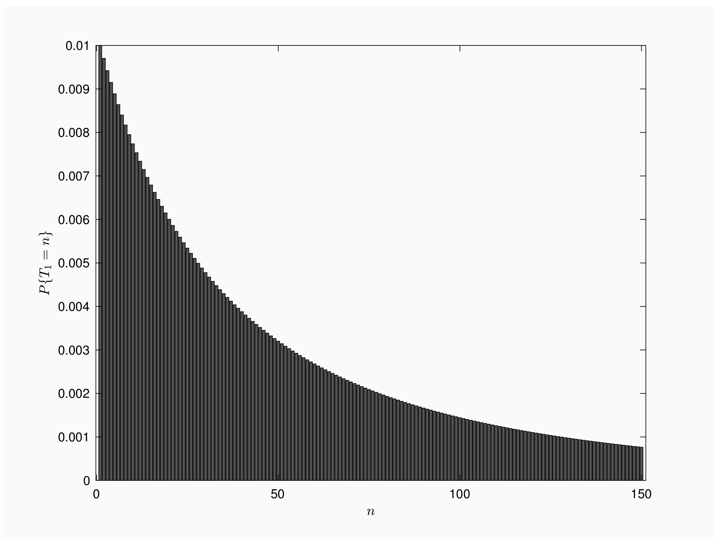
Figure 1 is a bar chart of $P\{T_1=n\},$ for $n\ge 1$. We consider a population of $N=100$ individuals and time interval between inspections is $\Delta t=0.01$ time units. Mass function presents a decreasing shape, with a single mode for $n=1$. From numerical results, we get that 1% of the outbreaks end by the time of the first inspection, but also 1% of the outbreaks will last more than 30,000 inspections.

Table 1. Cumulative probabilities for different population sizes.

	$\mathit{N}=5$	$\mathit{N}=25$	$\mathit{N}=50$	$\mathit{N}=75$
$P\{T_1\le 1\}$	$0.01$	$0.01$	$0.01$	$0.01$
$P\{T_1\le 10\}$	$0.0894$	$0.0882$	$0.0880$	$0.0880$
$P\{T_1\le 20\}$	$0.1599$	$0.1558$	$0.1553$	$0.1552$
$P\{T_1\le 30\}$	$0.2172$	$0.2093$	$0.2083$	$0.2080$
$P\{T_1\le 50\}$	$0.3047$	$0.2879$	$0.2858$	$0.2852$
$P\{T_1\le 75\}$	$0.3827$	$0.3536$	$0.3501$	$0.3489$
$P\{T_1\le 100\}$	$0.4400$	$0.3983$	$0.3932$	$0.3916$
$P\{T_1\le 125\}$	$0.4856$	$0.4302$	$0.4236$	$0.4215$
$P\{T_1\le 150\}$	$0.5226$	$0.4539$	$0.4458$	$0.4431$
$m_1$	$294.66$	$7094.24$	$582627.67$	$58366793.08$

displays several cumulative probabilities up to 150 inspections and the expected value $m_1$, for a population of $N=5,25,50$ and 75 individuals. We keep rates $\alpha =2.0$, $\gamma =1.0$ and time interval length as $\Delta t=0.01.$ For each population, only 1% of the outbreaks are inspected once before extinction. For a fixed number of inspections, cumulative probabilities are smaller when population size is larger. During outbreaks, large populations are inspected more times, in average, than smaller ones. Even for a small population of 5 individuals, we observe that the 48% of the outbreaks are still in progress at the 150-th inspection and an average of around 295 inspections take place while the epidemic is active.

Next, we describe the distribution of $T_1$ using a Box-Whiskers plot diagram. The objective is to compare the patterns of the number of inspections when we vary the contact rate. The box encloses the middle central part of the distribution, lower and upper edges of the box correspond to the lower and the upper quartile, respectively, and the line drawn across the box shows the median of the distribution. Finally, whiskers below start at 1 and whiskers above the boxes reach up to the 99% of the distribution.

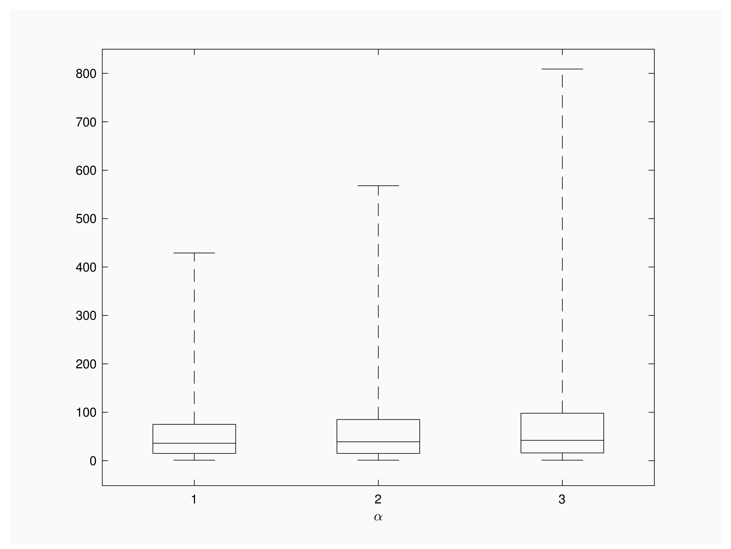
Figure 2 shows the distribution of $T_1$ for $\alpha =0.5,1.0$ and $2.0$. We consider a recovery rate $\gamma =2.0,$ a population of $N=20$ individuals and a time interval of $\Delta t=0.01$ units length between successive inspections. The distribution of the random variable is skewed to the right and longer right tails are observed for larger contact rates. Additional numerical results for $\gamma =5.0$ show a similar shape for box plot diagrams, with 99th quantile under 200 inspections. This fact is according to the intuition, because large recovery rates give more chance to recoveries than to new infections and, consequently, outbreaks will involve lesser infective individuals and present shorter extinction times in comparison with Figure 2’s scenario.

In

Table 2. Expected inspections before extinction time.

	$\mathit{\alpha }=0.5$	$\mathit{\alpha }=1.0$	$\mathit{\alpha }=2.0$	$\mathit{\alpha }=5.0$
$\gamma =0.5$	$444.73$	$6242.14$	$1.294\times {10}^7$	$1.917\times {10}^{13}$
$\gamma =1.0$	$134.19$	$222.36$	$3121.07$	$1.536\times {10}^8$
$\gamma =2.0$	$56.99$	$67.09$	$111.18$	$11,325.60$
$\gamma =5.0$	$21.01$	$22.16$	$25.02$	$44.47$

, we display the expected number of inspections for outbreaks starting from a single infective case, we consider several values for contact and recovery rates. Population contains 20 individuals and time interval between inspections is $\Delta t=0.01$, for every pair of rates. As was stated on Remark 4, results show that expected values are not a function of the basic reproductive number $R_0=\alpha /\gamma$. The expected number of inspections prior the end of the infective outbreak increases as a function of contact rate $\alpha$ and decreases as a function of recovery rate. That remark is according to the intuition too, because the epidemic length enlarges when contacts between individuals occur more often and/or when individuals need longer times to be recovered.

Next we focus on outbreaks that are first observed when the epidemic process involves i, not necessarily one, infected. Our aim is to describe the expected values $m_i$ when varying the initial number of infective individuals. Notice that Equation (20) guarantees that $m_i\ge m_{i-1}$, for $1<i\le N$. Thus, the expected number of inspections taking place prior to the epidemics end is a non-decreasing function regarding the amount of initial infective.

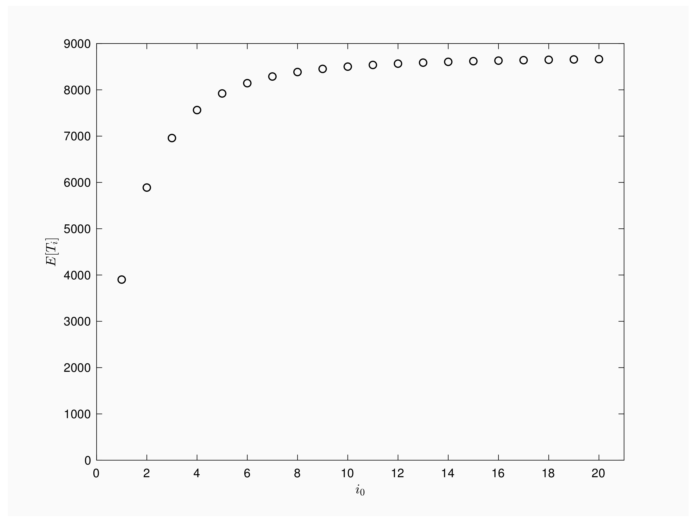
Figure 3 provides a numerical illustration for a population of $N=20$, contact rate $\alpha =1.8$, recovery rate $\gamma =0.8$ and time interval between periodic inspections $\Delta t=0.01.$ Pictured graph agrees with theoretical results, it quantifies the growth of the number of inspections when infective rises and it shows the importance of an early detection of such a epidemic process. More specifically, outbreaks detected at the first infection will be active, in mean terms, about 4000 inspections while if the outbreak is first checked when two infected are present in the population then, the expected inspections will rise up to 6000 times or up to 8000 inspections when first checking shows five infected.

Additional numerical results, not included here, report that when we choose intervals between inspections with decreasing length $\Delta t$, the mass distribution function of any $T_i$, for $1\le i\le N$, provides an aproximation to the density function of the extinction time of an epidemic process starting with i infected [28], that is the continuous counterpart of the number of periodic inspections taking place while the epidemic process is active.

In the following section we present a possible use of the probabilistic behavior of $T_i=\left(T\right|I_0=i).$

4.2. Application to Evaluate Outbreak Benefits

Let us assume that every inspection has a travel or approaching cost $c_1$ and, whenever there is a change in the population regarding the immediate previous inspection, we get a profit in terms of information that depends on the type of event. Let $g_R$ and $g_I$ represent recovery and infection detection’s gain, respectively.

Associated to every outbreak, the random variable $T_i$ provides the total number of inspections conducted during an outbreak that starts from $I_0=i$ infective individuals. On the other hand, for outbreaks starting with $I_0=i$ infective individuals, Artalejo et al. introduced in [30] the random variables $N_i^R$ and $N_i^I$ defined as the number of recoveries and infections per outbreak, respectively. By noticing that the number of recoveries in an outbreak agrees with the total number of infections in the same outbreak, we get

$$N_i^R=i+N_i^I,\mathrm{for}i\ge 1.$$

(21)

With the help of the above random variables and its relationship (21), we can determine outbreak’s benefit, for instance, just by defining a benefit function conditioned to the initial number of infective, as follows

$$B(T,R|I_0=i)=(g_R+g_I)N_i^R-i{g}_I-c_1{T}_i.$$

(22)

The expected benefit per outbreak will depend on the mean values of $N_i^R$ and $T_i$, but also on the choice of travel cost and information profits.

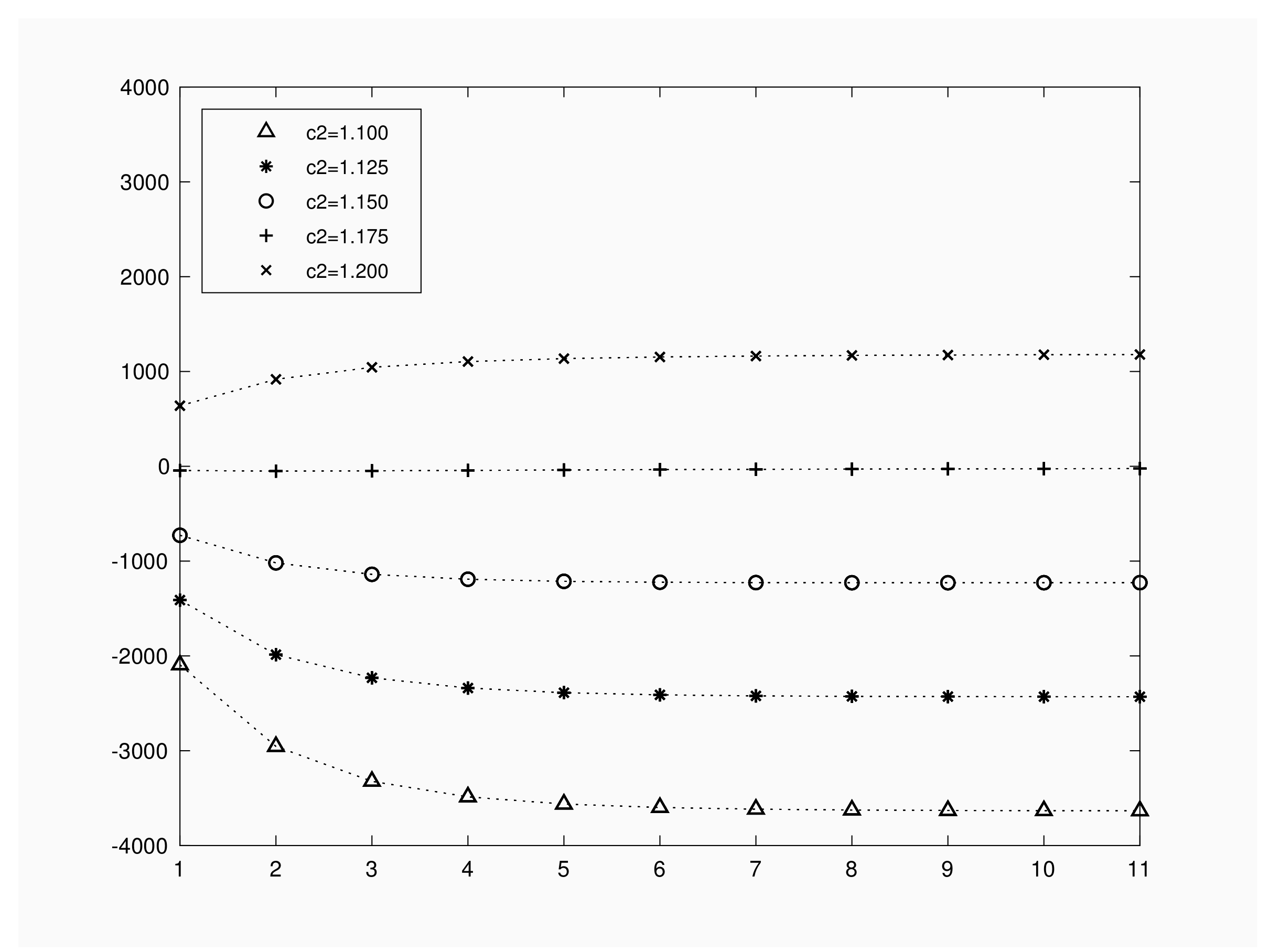
Figure 4 represents expected benefit when the initial number of infective varies in $1\le i\le 11$, for a population of $N=25$, with contact rate $\alpha =2.5$, recovery rate of $\gamma =1.0$ and a time interval of $\Delta t=0.01$ units. We fixed a unitary travel cost per the inspection; i.e. $c_1=1$, and gain values per recovery or infection have been chosen as $g_R=g_I=c_2$. Several graphs are drawn by fixing $c_2>c_1$. We notice first that, for a fixed number of infective and in order to obtain a positive benefit, recovery gain $c_2$ must satisfy $c_2>c_{1}E\left[T_i\right]/(2E\left[N_i^R\right]-i)$. Hence, the trivial restriction $c_2>c_1$ does not guarantee a positive expected benefit per outbreak. In any case, the expected benefit is a linear increasing function of the gain value $c_2$.

As we can see in Figure 4, depending on the choice for $c_2$, expected benefit functions present different shape as a function of the initial number of infective individuals. Numerical results show that, for $c_2\le 1.125$, expected benefit decreases as the initial infected increases. For $c_2=1.15$ we obtain a minimum expected benefit at $I_0=9$ infective. When we set $c_2=1.175$ the minimum corresponds to the value $I_0=2$ but we obtain expected values close to 0. For $c_2\ge 1.2$, expected benefit remains almost constant for $I_0\ge 5$. These facts illustrate that a deep knowledge on $E\left[N_i^R\right]$ or $E\left[T_i\right]$ will help in decision making process regarding travel cost and gain values.

5. Discussion and Conclusions

Literature in mathematical modelization of epidemics includes both continuous and discrete-time models. Continuous-time models are more accurate but more difficult to implement than discrete-time ones. On the other hand, discrete-time models fit better with real information; data related to real-world epidemic processes are often given by unit time, so it is natural to preserve dynamic features by modeling a dynamical system from observations at discrete times which are adapted to time step.

This paper focuses on the discrete-time SIS model, where transition probabilities for event occurring during time-steps are described in terms of an absorbing DTMC. The population is observed at periodic time points assuming that at most one event takes in a time-step. The discrete-time stochastic epidemic SIS models are formulated as DTMC which may be considered approximations to the continuous-time Markov jump processes. The size of the time step must be controlled to assure that the model gives genuine probability distributions.

Our purpose is to study the extinction time counterpart in discrete-time, that is the random variable that counts the total number of inspections that find an active epidemic process.

Subject to the initial number of infective individuals, mass probability function of the number of inspections, $T_i$, is numerically determined through a recursive scheme; complementing the probabilistic knowledge of this variable provided by its expected value, that comes directly from an explicit expression.

A really interesting extension of this work arises when considering equidistant time inspections relaxing the requirement about the maximum number of events observed during inspections. This problem, that appears to be analytically intractable, is the aim of the paper [31], where authors tackle this difficulty via the total area between the sample paths of the numbers of infective individuals in the continuous-time process and its discrete-time counterpart.

References

- Bailey, N.T.J. The Mathematical Theory of Infectious Diseases; Griffin & Co.: New York, NY, USA, 1975; ISBN 0852642318, 9780852642313. [Google Scholar]
- Andersson, H.; Britton, T. Stochastic Epidemic Models And Their Statistical Analysis; Lectures Notes in Statistics; Springer: New York, NY, USA, 2000; Volume 151, ISBN 978-1-4612-1158-7. [Google Scholar]
- Becker, N.G. Analysis of Infectious Disease Data; Chapman & Hall/CRC: Boca Raton, FL, USA, 2000; ISBN 0-412-30990-4. [Google Scholar]
- Kawachi, K. Deterministic models for rumor transmission. Nonlinear Anal. Real World Appl. 2008, 9, 1989–2028. [Google Scholar] [CrossRef]
- Isham, V.; Harden, S.; Nekovee, M. Stochastic epidemics and rumours on finite random networks. Phys. A Stat. Mech. Appl. 2010, 389, 561–576. [Google Scholar] [CrossRef]
- Amador, J.; Artalejo, J.R. Stochastic modeling of computer virus spreading with warning signals. J. Frankl. Inst. 2013, 350, 1112–1138. [Google Scholar] [CrossRef]
- De Martino, G.; Spina, S. Exploiting the time-dynamics of news diffusion on the Internet through a generalized Susceptible-Infected model. Phys. A Stat. Mech. Appl. 2015, 438, 634–644. [Google Scholar] [CrossRef]
- Giorno, V.; Spina, S. Rumor spreading models with random denials. Phys. A Stat. Mech. Appl. 2016, 461, 569–576. [Google Scholar] [CrossRef]
- Britton, T. Stochastic epidemic models: A survey. Math. Biosci. 2010, 225, 24–35. [Google Scholar] [CrossRef] [PubMed] [Green Version]
- Diekman, O.; Heesterbeek, H.; Britton, T. Mathematical for Understanding Infectious Disease Dynamics; Princeton University Press: Princeton, NJ, USA, 2012; ISBN 9781400845620. [Google Scholar]
- Van den Driessche, P. Reproduction numbers of infectious disease models. Infect. Dis. Model 2017, 2, 288–303. [Google Scholar] [CrossRef] [PubMed]
- Artalejo, J.R.; Lopez-Herrero, M.J. On the exact measure of disease spread in stochastic epidemic models. Bull. Math. Biol. 2013, 75, 1031–1050. [Google Scholar] [CrossRef] [PubMed]
- Lopez-Herrero, M.J. Epidemic transmission on SEIR stochastic models with nonlinear incidence rate. Math. Methods Appl. Sci. 2016, 40, 2532–2541. [Google Scholar] [CrossRef] [Green Version]
- Emmert, K.E.; Allen, L.J.S. Population persistence and extinction in a discrete-time, stage-structured epidemic model. J. Differ. Equ. Appl. 2004, 10, 1177–1199. [Google Scholar] [CrossRef]
- Allen, L.J.S.; van den Driessche, P. The basic reproduction number in some discrete-time epidemic models. J. Differ. Equ. Appl. 2008, 14, 1127–1147. [Google Scholar] [CrossRef]
- Li, J.Q.; Lou, J.; Lou, M.Z. Some discrete SI and SIS epidemic models. Appl. Math. Mech. 2008, 29, 113–119. [Google Scholar] [CrossRef]
- Zhang, J.; Jin, Z. Discrete time SI and SIS epidemic models with vertical transmission. J. Biol. Syst. 2009, 17, 201–212. [Google Scholar] [CrossRef]
- Farnoosh, R.; Parsamanesh, M. Disease extinction and persistence in a discrete-time SIS epidemic model with vaccination and varying population size. Filomat 2017, 31, 4735–4747. [Google Scholar] [CrossRef]
- d’Onofrio, A.; Manfredi, P.; Salinelli, E. Dynamic behaviour of a discrete-time SIR model with information dependent vaccine uptake. J. Differ. Equ. Appl. 2016, 22, 485–512. [Google Scholar] [CrossRef]
- Tuckell, H.C.; Williams, R.J. Some properties of a simple stochastic epidemic model of SIR type. Math. Biosci. 2007, 208, 76–97. [Google Scholar] [CrossRef] [PubMed]
- Ferrante, M.; Ferraris, E.; Rovira, C. On a stochastic epidemic SEIHR model and its diffusion approximation. TEST 2016, 25, 482–502. [Google Scholar] [CrossRef]
- Van den Driessche, P.; Yakubu, A. Disease extinction versus persistence in discrete-time epidemic models. Bull. Math. Biol. 2018. [Google Scholar] [CrossRef] [PubMed]
- Allen, L.J.S.; van den Driessche, P. Relations between deterministic and stochastic thresholds for disease extinction in continuous- and discrete-time infectious disease models. Math. Biosci. 2013, 243, 99–108. [Google Scholar] [CrossRef] [PubMed]
- Fennell, P.G.; Melnik, S.; Gleeson, J.P. Limitations of discrete-time approaches to continuous-time contagion dynamics. Phys. Rev. E 2016, 94, 052125. [Google Scholar] [CrossRef] [PubMed]
- Norden, R.H. On the distribution of the time to extinction in the stochastic logistic population model. Adv. Appl. Probab. 1982, 14, 687–708. [Google Scholar] [CrossRef]
- Allen, L.J.S.; Burgin, A.M. Comparison of deterministic and stochastic SIS and SIR models in discrete time. Math. Biosci. 2000, 163, 1–33. [Google Scholar] [CrossRef] [Green Version]
- Stone, P.; Wilkinson-Herbots, H.; Isham, V. A stochastic model for head lice infections. J. Math. Biol. 2008, 56, 743–763. [Google Scholar] [CrossRef] [PubMed]
- Artalejo, J.R.; Economou, A.; Lopez-Herrero, M.J. Stochastic epidemic models revisited: Analysis of some continuous performance measures. J. Biol. Dyn. 2012, 6, 189–211. [Google Scholar] [CrossRef] [PubMed] [Green Version]
- Kulkarni, V.G. Modeling and Analysis of Stochastic Systems; Chapman & Hall: London, UK, 1995; ISBN 0-412-04991-0. [Google Scholar]
- Artalejo, J.R.; Economou, A.; Lopez-Herrero, M.J. On the number of recovered individuals in the SIS and SIR stochastic epidemic models. Math. Biosci. 2010, 228, 45–55. [Google Scholar] [CrossRef] [PubMed]
- Gómez-Corral, A.; López-García, M.; Rodríguez-Bernal, M.T. On time-discretized versions of SIS epidemic models. 2018; in press. [Google Scholar]
Figure 1.
Mass function for .
Figure 2.
Box plot for .
Figure 3.
Expected number of inspections versus initial infective.
Figure 4.
Expected Benefit versus initial infective.