A High Accurate and Stable Legendre Transform Based on Block Partitioning and Butterfly Algorithm for NWP

Abstract

In this paper, we proposed a high accurate and stable Legendre transform algorithm, which can reduce the potential instability for a very high order at a very small increase in the computational time. The error analysis of interpolative decomposition for Legendre transform is presented. By employing block partitioning of the Legendre-Vandermonde matrix and butterfly algorithm, a new Legendre transform algorithm with computational complexity O(Nlog²N /loglogN) in theory and O(Nlog³N) in practical application is obtained. Numerical results are provided to demonstrate the efficiency and numerical stability of the new algorithm.

1. Introduction

Legendre transform (LT) plays an important part in many scientific applications, such as astrophysical [1], numerical weather prediction and climate models [2,3]. Fast Legendre transform attracts considerable interest amongst the scientific computing and numerical simulation. Scientists have paid very serious attention to develop fast Legendre transform algorithms [4,5,6,7,8,9,10,11]. The validity and reliability of these algorithms depend on whether they can keep fast, stable and high accuracy.

The butterfly algorithm [12,13] is an effective multilevel technique to compress a matrix that satisfies a complementary low-rank property. It factorizes a complementary low-rank matrix K of size N×N into the product of O(logN) sparse matrices, each with O(N) nonzero entries. Hence, dense matrix-vector multiplication can be transformed into a set of sparse matrix-vector multiplication in O(NlogN) operations [14]. LT using butterfly algorithm has the advantages of high accuracy, stability and low computational complexity.

As one of the most widely used butterfly algorithms, Tygert’s algorithm (2010) [11] has been successfully implemented in IFS of ECMWF [2], YHGSM [15,16,17] of NUDT [3] and astrophysical [1]. In the applications of numerical weather prediction and climate models, which need spectral harmonic transform (SHT) many times for each time step, only one precomputation is needed in the first-time step, then the results are stored in memory and reused in each transform. Though Tygert’s algorithm (2010) is slow in terms of precomputation: O(N²) for LT and O(N³) for SHT, it does not have much impact on total performance. However, some unsolved issues still remain. The main issue is the potential instability of interpolative decomposition (ID) [18] for very high order Legendre transform. That said, Tygert [11] points out that the reason why the butterfly procedure works so well for associated Legendre functions may be that the associated transforms nearly weighted averages of Fourier integral operators. There are no literatures to prove that the pre-computations will compress the appropriate N × N matrix enough to enable application of the matrix to vectors using only O(NlogN) floating-point operations(flops). Full numerical stability has been demonstrated both empirically and theoretically for fast Fourier transform (FFT) using butterfly algorithm. It is difficult to give complete and rigorous proofs of interpolative decomposition for Legendre transform as Fourier transform.

Non-oscillatory phase functions method opens up new avenues for special function transforms. The solutions of some kinds of second order differential equations can be accurately represented by non-oscillatory phase functions [19,20]. It has been proved that Legendre’s differential equation [21] and its generalization Jacobi’s differential equation [22] admit a non-oscillatory phase function. So non-oscillatory phase functions can be used to the expansions [22], the calculation of the roots [23] and transform [24] of special functions. Jacobi transform by non-oscillatory phase functions shows an optimal computational complexity O(Nlog²N/loglogN) in reference [24]. However, Legendre transform algorithm in ButterflyLab [25], which adopts interpolative butterfly factorization (IBF) [14,26] and non-oscillatory phase functions method to evaluate the Legendre polynomials [24], does not show high accuracy as Fourier transform using IBF. Therefore, Fast Legendre transform (FLT) based on IBF and non-oscillatory phase functions and its extension to the associated Legendre functions need further study.

Recently, fast Legendre transform algorithm based on FFT deserved more attentions for its optimal computational complexity O(Nlog²N/loglogN). Hale and Townsend [27] firstly presented a fast Chebyshev-Legendre transform, and then developed a non-uniform discrete cosine transform which use a Taylor series expansion for Chebyshev polynomials about equally-spaced points in the frequency domain. Finally, Hale and Townsend [28] got an O(Nlog²N /loglogN) Legendre transform algorithm. In the near future, fast polynomial transforms [29] based on Toeplitz and Hankel matrices will be presented to accelerate the Chebyshev-Legendre transform. Although FFT-based LT has the attractive computational complexity, it needs too many times FFT, which makes FFT-based LT only become more computationally efficient than LT using Dgemv when N is greater than or equal to 5000. Since the computation of associated-Legendre-Vandermonde matrices is completed in the pre-computation step, it will become worse on the occasion of multiple use of FLT such as NWP, in which only once computation of associated-Legendre-Vandermonde matrices is needed for many times spectral harmonic transform (SHT).

Motivated and inspired by the ongoing research in these areas, we present a theoretical method to analyze the error of LT using butterfly algorithm, and then provide a numerically stability Legendre transform algorithm based on block partitioning and butterfly algorithm. The novel aspect is the mitigation of the potential instability of LT using butterfly algorithm at a very small increase of computational cost.

2. Mathematical Preliminaries

In this section, we introduce the theorem that Legendre polynomials on equally-spaced grid can be expressed as a weighted linear combination of Chebyshev polynomials, and a partitioning of Legendre-Vandermonde matrix $P_{\mathrm{N}}\left(x_N^{cheb}\right)$ ($x={\underset{\_}{x}}_N^{cheb}=\cos \left({\underset{\_}{\theta }}_N^{cheb}\right)$). For more details, see references [27,28].

According to Stieltjes’s theory [30], Legendre polynomials can be expressed as following asymptotic formula when $n\to \infty$

$$P_n\left(\cos \theta \right)=C_n{\displaystyle \sum _{m=0}^{M-1}{h}_{m,n}\frac{\cos \left(\left(m+n+\frac{1}{2}\right)\theta -\left(m+\frac{1}{2}\right)\frac{\pi }{2}\right)}{{\left(2\sin \theta \right)}^{m+1/2}}}+R_{M,n}\left(\theta \right)$$

(1)

where $\theta ={\cos }^{-1}x$, $\theta \in \left(0,\pi \right)$ and

$$C_n=\frac{4}{\pi }{\displaystyle \prod _{j=1}^n\frac{j}{j+1/2}}=\sqrt{\frac{4}{\pi }}\frac{\Gamma \left(n+1\right)}{\Gamma \left(n+3/2\right)}$$

(2)

$$h_{m,n}=\{\begin{array}{cc}1,& m=0,\\ {\displaystyle {\prod }_{j=1}^m\frac{{\left(j-1/2\right)}^2}{j\left(n+j+1/2\right)}},& m>0.\end{array}$$

(3)

The error term in Equation (1) can be bounded by

$$\left|R_{M,n}\left(\theta \right)\right|\le C_n{h}_{M,n}\frac{2}{{\left(2\sin \theta \right)}^{M+1/2}}$$

(4)

Hale and Townsend [27] rewrote Equation (1) as a weighted linear combination of Chebyshev polynomials

$$P_n\left(\cos \theta \right)=C_n{\displaystyle \sum _{m=0}^{M-1}{h}_{m,n}\left(u_m\left(\theta \right)T_n\left(\sin \theta \right)+v_m\left(\theta \right)T_n\left(\cos \theta \right)\right)}+R_{M,n}\left(\theta \right)$$

(5)

with $T_n\left(\cos \theta \right)=\cos \left(n\theta \right)$, $T_n\left(\sin \theta \right)=\sin \left(n\theta \right)$ and

$$u_m\left(\theta \right)=\frac{\sin \left(\left(m+1/2\right)\left(\frac{\pi }{2}-\theta \right)\right)}{{\left(2\sin \theta \right)}^{m+1/2}},v_m\left(\theta \right)=\frac{\cos \left(\left(m+1/2\right)\left(\frac{\pi }{2}-\theta \right)\right)}{{\left(2\sin \theta \right)}^{m+1/2}}$$

(6)

Let $x_k^{leg}=\cos \left({\theta }_k^{leg}\right)$ and ${\theta }_0^{leg},\cdots ,{\theta }_{N-1}^{leg}$ are the transformed Legendre nodes, Equation (5) can be written as

$$P_n\left(x_k^{leg}\right)=C_n{\displaystyle \sum _{m=0}^{M-1}{h}_{m,n}\left(u_m\left({\theta }_k^{leg}\right)T_n\left(\sin \left({\theta }_k^{leg}\right)\right)+v_m\left({\theta }_k^{leg}\right)T_n\left(\cos \left({\theta }_k^{leg}\right)\right)\right)}+R_{M,n}\left({\theta }_k^{leg}\right)$$

(7)

3. Error Analysis of Legendre Transform using Butterfly Algorithm

The transformed Legendre nodes ${\theta }_0^{leg},\cdots ,{\theta }_{N-1}^{leg}$ can be seen as a perturbation of an equally-spaced grid ${\theta }_0^{\ast },\cdots ,{\theta }_{N-1}^{\ast }$, i.e

$${\theta }_k^{leg}={\theta }_k^{*}+\delta {\theta }_k,\hspace{1em}0\le k\le N-1$$

(8)

and then approximate each $x_k^{leg}=\cos \left(n{\theta }_k^{leg}\right)$ term by a truncated Taylor series expansion about ${\theta }_k^{*}$. If $\left|\delta {\theta }_k\right|$ is small then only a few terms in the Taylor expansion are required.

The Taylor series expansion of $T_n\left(\cos \left(\theta +\delta \theta \right)\right)=\cos \left(n\left(\theta +\delta \theta \right)\right)$ about $\theta \in \left[0,\pi \right]$ can be expressed as

$$\begin{array}{ll}\cos \left(n\left(\theta +\delta \theta \right)\right)& =\cos \left(n\theta \right)+{\displaystyle \sum _{l=1}^{\infty }{\cos }^{\left(l\right)}\left(n\theta \right)\frac{{\left(n\delta \theta \right)}^l}{l!}}\\ & =\cos \left(n\theta \right)+{\displaystyle \sum _{l=1}^{\infty }{\left(-1\right)}^{\lfloor \left(l+1\right)/2\rfloor }{\Phi }_l\left(n\theta \right)\frac{{\left(n\delta \theta \right)}^l}{l!}}\end{array}$$

(9)

where

$${\Phi }_l\left(\theta \right)=\{\begin{array}{lll}\cos \left(\theta \right),& l& even\\ \sin \left(\theta \right),& l& odd\end{array}$$

(10)

Similarly, $T_n\left(\sin \left(\theta +\delta \theta \right)\right)=\sin \left(n\left(\theta +\delta \theta \right)\right)$ about $\theta \in \left[0,\pi \right]$ can be expressed as

$$\begin{array}{ll}\sin \left(n\left(\theta +\delta \theta \right)\right)& =\sin \left(n\theta \right)+{\displaystyle \sum _{l=1}^{\infty }{\sin }^{\left(l\right)}\left(n\theta \right)\frac{{\left(n\delta \theta \right)}^l}{l!}}\\ & =\sin \left(n\theta \right)+{\displaystyle \sum _{l=1}^{\infty }{\left(-1\right)}^{\lfloor l/2\rfloor }{\Psi }_l\left(n\theta \right)\frac{{\left(n\delta \theta \right)}^l}{l!}}\end{array}$$

(11)

where

$${\Psi }_l\left(\theta \right)=\{\begin{array}{lll}\cos \left(\theta \right),& l& odd\\ \sin \left(\theta \right),& l& even\end{array}$$

(12)

Substituting ${\theta }_k^{*}$ for $\theta$ in Equation (5), one can get

$$\begin{array}{ll}{P}_n\left(\cos \left({\theta }_k^{\ast }\right)\right)=& C_n{T}_n\left(\sin \left({\theta }_k^{\ast }\right)\right){\displaystyle \sum _{m=0}^{M-1}{h}_{m,n}{u}_m\left({\theta }_k^{\ast }\right)}\\ & +C_n{T}_n\left(\cos \left({\theta }_k^{\ast }\right)\right){\displaystyle \sum _{m=0}^{M-1}{h}_{m,n}{v}_m\left({\theta }_k^{\ast }\right)}+R_{M,n}\left({\theta }_k^{\ast }\right)\end{array}$$

(13)

The Taylor series expansion of $P_n\left(\cos \left({\theta }_k^{leg}\right)\right)$ about ${\theta }_k^{\ast }$ can be expressed as

$$P_n\left(\cos \left({\theta }_k^{leg}\right)\right)=P_n\left(\cos \left({\theta }_k^{\ast }+\delta {\theta }_k\right)\right)={\displaystyle \sum _{l=0}^{\infty }{P}_n^{\left(l\right)}\left(\cos \left({\theta }_k^{\ast }\right)\right)\frac{{\left(\delta {\theta }_k\right)}^l}{l!}}$$

(14)

According to Equation (13), $P_n^{\left(l\right)}\left(\cos \left({\theta }_k^{\ast }\right)\right)$ ($l>0$) can be written as

$$\begin{array}{ll}{P}_n^{\left(l\right)}\left(\cos \left({\theta }_k^{\ast }\right)\right)=& C_n{\displaystyle \sum _{m=0}^{M-1}{h}_{m,n}\left\{u_m\left({\theta }_k^{\ast }\right)T_n^{\left(l\right)}\left(\sin \left({\theta }_k^{\ast }\right)\right)+u_m^{\left(l\right)}\left({\theta }_k^{\ast }\right)T_n\left(\sin \left({\theta }_k^{\ast }\right)\right)\right\}}\\ & +C_n{\displaystyle \sum _{m=0}^{M-1}{h}_{m,n}\left\{v_m\left({\theta }_k^{\ast }\right)T_n^{\left(l\right)}\left(\cos \left({\theta }_k^{\ast }\right)\right)+v_m^{\left(l\right)}\left({\theta }_k^{\ast }\right)T_n\left(\cos \left({\theta }_k^{\ast }\right)\right)\right\}}\\ & +R_{M,n}^l\left({\theta }_k^{\ast }\right)\end{array}$$

(15)

Substituting Equation (15) into Equation (14), one can obtain

$$\begin{array}{ll}{P}_n\left(x_k^{leg}\right)=& C_n{\displaystyle \sum _{m=0}^{M-1}{h}_{m,n}\left\{u_m\left({\theta }_k^{\ast }\right)T_n\left(\sin \left({\theta }_k^{\ast }\right)\right)+v_m\left({\theta }_k^{\ast }\right)T_n\left(\cos \left({\theta }_k^{\ast }\right)\right)\right\}}\\ & +C_n{\displaystyle \sum _{l=1}^{\infty }\frac{{\left(\delta {\theta }_k\right)}^l}{l!}{\displaystyle \sum _{m=0}^{M-1}{h}_{m,n}\left\{u_m\left({\theta }_k^{\ast }\right)T_n^{\left(l\right)}\left(\sin \left({\theta }_k^{\ast }\right)\right)+u_m^{\left(l\right)}\left({\theta }_k^{\ast }\right)T_n\left(\sin \left({\theta }_k^{\ast }\right)\right)\right\}}}\\ & +C_n{\displaystyle \sum _{l=1}^{\infty }\frac{{\left(\delta {\theta }_k\right)}^l}{l!}{\displaystyle \sum _{m=0}^{M-1}{h}_{m,n}\left\{v_m\left({\theta }_k^{\ast }\right)T_n^{\left(l\right)}\left(\cos \left({\theta }_k^{\ast }\right)\right)+v_m^{\left(l\right)}\left({\theta }_k^{\ast }\right)T_n\left(\cos \left({\theta }_k^{\ast }\right)\right)\right\}}}\\ & +{\displaystyle \sum _{l=0}^{\infty }{R}_{M,n}^{\left(l\right)}\left({\theta }_k^{\ast }\right)\frac{{\left(\delta {\theta }_k\right)}^l}{l!}}\end{array}$$

(16)

Because

$$\begin{array}{ll}{\displaystyle \sum _{l=0}^{\infty }\frac{{\left(\delta {\theta }_k\right)}^l}{l!}{T}_n\left(\sin \left({\theta }_k^{\ast }\right)\right){\displaystyle \sum _{m=0}^{M-1}{h}_{m,n}{u}_m^{\left(l\right)}\left({\theta }_k^{\ast }\right)}}& =T_n\left(\sin \left({\theta }_k^{\ast }\right)\right){\displaystyle \sum _{m=0}^{M-1}{h}_{m,n}{\displaystyle \sum _{l=0}^{\infty }{u}_m^{\left(l\right)}\left({\theta }_k^{\ast }\right)\frac{{\left(\delta {\theta }_k\right)}^l}{l!}}}\\ & =T_n\left(\sin \left({\theta }_k^{\ast }\right)\right){\displaystyle \sum _{m=0}^{M-1}{h}_{m,n}{u}_m\left({\theta }_k^{\ast }+\delta {\theta }_k\right)}\\ & =T_n\left(\sin \left({\theta }_k^{\ast }\right)\right){\displaystyle \sum _{m=0}^{M-1}{h}_{m,n}{u}_m\left({\theta }_k^{leg}\right)}\end{array}$$

(17)

and

$$\begin{array}{ll}{\displaystyle \sum _{l=0}^{\infty }\frac{{\left(\delta {\theta }_k\right)}^l}{l!}{T}_n\left(\cos \left({\theta }_k^{\ast }\right)\right){\displaystyle \sum _{m=0}^{M-1}{h}_{m,n}{v}_m^{\left(l\right)}\left({\theta }_k^{\ast }\right)}}& =T_n\left(\cos \left({\theta }_k^{\ast }\right)\right){\displaystyle \sum _{m=0}^{M-1}{h}_{m,n}{\displaystyle \sum _{l=0}^{\infty }{v}_m^{\left(l\right)}\left({\theta }_k^{\ast }\right)\frac{{\left(\delta {\theta }_k\right)}^l}{l!}}}\\ & =T_n\left(\cos \left({\theta }_k^{\ast }\right)\right){\displaystyle \sum _{m=0}^{M-1}{h}_{m,n}{v}_m\left({\theta }_k^{\ast }+\delta {\theta }_k\right)}\\ & =T_n\left(\cos \left({\theta }_k^{\ast }\right)\right){\displaystyle \sum _{m=0}^{M-1}{h}_{m,n}{v}_m\left({\theta }_k^{leg}\right)}\end{array}$$

(18)

Similarly, we have

$$\begin{array}{ll}{\displaystyle \sum _{l=0}^{\infty }\frac{{\left(\delta {\theta }_k\right)}^l}{l!}{\displaystyle \sum _{m=0}^{M-1}{h}_{m,n}{u}_m\left({\theta }_k^{\ast }\right)T_n^{\left(l\right)}\left(\sin \left({\theta }_k^{\ast }\right)\right)}}& ={\displaystyle \sum _{m=0}^{M-1}{h}_{m,n}{u}_m\left({\theta }_k^{\ast }\right){\displaystyle \sum _{l=0}^{\infty }{T}_n^{\left(l\right)}\left(\sin \left({\theta }_k^{\ast }\right)\right)\frac{{\left(\delta {\theta }_k\right)}^l}{l!}}}\\ & ={\displaystyle \sum _{m=0}^{M-1}{h}_{m,n}{u}_m\left({\theta }_k^{\ast }\right)T_n\left(\sin \left({\theta }_k^{leg}\right)\right)}\end{array}$$

(19)

and

$$\begin{array}{ll}{\displaystyle \sum _{l=0}^{\infty }\frac{{\left(\delta {\theta }_k\right)}^l}{l!}{\displaystyle \sum _{m=0}^{M-1}{h}_{m,n}{v}_m\left({\theta }_k^{\ast }\right)T_n^{\left(l\right)}\left(\cos \left({\theta }_k^{\ast }\right)\right)}}& ={\displaystyle \sum _{m=0}^{M-1}{h}_{m,n}{v}_m\left({\theta }_k^{\ast }\right){\displaystyle \sum _{l=0}^{\infty }{T}_n^{\left(l\right)}\left(\cos \left({\theta }_k^{\ast }\right)\right)\frac{{\left(\delta {\theta }_k\right)}^l}{l!}}}\\ & ={\displaystyle \sum _{m=0}^{M-1}{h}_{m,n}{v}_m\left({\theta }_k^{\ast }\right)T_n\left(\cos \left({\theta }_k^{leg}\right)\right)}\end{array}$$

(20)

Substituting Equations (17)–(20) into Equation (16), one can get

$$\begin{array}{ll}{P}_n\left(x_k^{leg}\right)=& C_n{\displaystyle \sum _{m=0}^{M-1}{h}_{m,n}\left(u_m\left({\theta }_k^{leg}\right)T_n\left(\sin \left({\theta }_k^{\ast }\right)\right)+v_m\left({\theta }_k^{leg}\right)T_n\left(\cos \left({\theta }_k^{\ast }\right)\right)\right)}\\ & +C_n{\displaystyle \sum _{m=0}^{M-1}{h}_{m,n}\left\{u_m\left({\theta }_k^{\ast }\right)T_n\left(\sin \left({\theta }_k^{leg}\right)\right)+v_m\left({\theta }_k^{\ast }\right)T_n\left(\cos \left({\theta }_k^{leg}\right)\right)\right\}}\\ & -C_n{\displaystyle \sum _{m=0}^{M-1}{h}_{m,n}\left\{u_m\left({\theta }_k^{*}\right)T_n\left(\sin \left({\theta }_k^{\ast }\right)\right)+v_m\left({\theta }_k^{*}\right)T_n\left(\cos \left({\theta }_k^{\ast }\right)\right)\right\}}\\ & +R_{M,n}\left({\theta }_k^{leg}\right)\end{array}$$

(21)

Then

$$\begin{array}{ll}{P}_n\left(x_k^{leg}\right)=& C_n{\displaystyle \sum _{m=0}^{M-1}{h}_{m,n}\left(u_m\left({\theta }_k^{leg}\right)T_n\left(\sin \left({\theta }_k^{\ast }\right)\right)+v_m\left({\theta }_k^{leg}\right)T_n\left(\cos \left({\theta }_k^{\ast }\right)\right)\right)}\\ & +C_n{\displaystyle \sum _{m=0}^{M-1}{h}_{m,n}\left\{u_m\left({\theta }_k^{\ast }\right)T_n\left(\sin \left({\theta }_k^{leg}\right)\right)+v_m\left({\theta }_k^{\ast }\right)T_n\left(\cos \left({\theta }_k^{leg}\right)\right)\right\}}\\ & -P_n\left(x_k^{*}\right)+R_{M,n}\left({\theta }_k^{*}\right)+R_{M,n}\left({\theta }_k^{leg}\right)\end{array}$$

(22)

By truncating the second term in the right hand side of Equation (19), it can be approximated as

$$\begin{array}{ll}{P}_n\left(x_k^{leg}\right)=& C_n{\displaystyle \sum _{m=0}^{M-1}{h}_{m,n}\left(u_m\left({\theta }_k^{leg}\right)T_n\left(\sin \left({\theta }_k^{\ast }\right)\right)+v_m\left({\theta }_k^{leg}\right)T_n\left(\cos \left({\theta }_k^{\ast }\right)\right)\right)}\\ & +C_n{\displaystyle \sum _{l=1}^L\frac{{\left(\delta {\theta }_k\right)}^l}{l!}{\displaystyle \sum _{m=0}^{M-1}{h}_{m,n}\left\{u_m\left({\theta }_k^{\ast }\right)T_n^{\left(l\right)}\left(\sin \left({\theta }_k^{\ast }\right)\right)+v_m\left({\theta }_k^{\ast }\right)T_n^{\left(l\right)}\left(\cos \left({\theta }_k^{\ast }\right)\right)\right\}}}\\ & +R_{M,n}\left({\theta }_k^{leg}\right)+R_{L,M,n,\delta \theta }\end{array}$$

(23)

and then

$$\begin{array}{ll}{P}_n\left(x_k^{leg}\right)=& C_n{\displaystyle \sum _{m=0}^{M-1}{h}_{m,n}\left(u_m\left({\theta }_k^{leg}\right)T_n\left(\sin \left({\theta }_k^{\ast }\right)\right)+v_m\left({\theta }_k^{leg}\right)T_n\left(\cos \left({\theta }_k^{\ast }\right)\right)\right)}\\ & +C_n{\displaystyle \sum _{l odd}^L\frac{{\left(n\delta {\theta }_k\right)}^l}{l!}{\displaystyle \sum _{m=0}^{M-1}{h}_{m,n}\left({\left(-1\right)}^{\lfloor \frac{l}{2}\rfloor }{u}_m\left({\theta }_k^{\ast }\right)T_n\left(\cos {\theta }_k^{\ast }\right)+{\left(-1\right)}^{\lfloor \frac{\left(l+1\right)}{2}\rfloor }{v}_m\left({\theta }_k^{\ast }\right)T_n\left(\sin {\theta }_k^{\ast }\right)\right)}}\\ & +C_n{\displaystyle \sum _{l even}^L\frac{{\left(n\delta {\theta }_k\right)}^l}{l!}{\displaystyle \sum _{m=0}^{M-1}{h}_{m,n}\left({\left(-1\right)}^{\lfloor \frac{l}{2}\rfloor }{u}_m\left({\theta }_k^{\ast }\right)T_n\left(\sin {\theta }_k^{\ast }\right)+{\left(-1\right)}^{\lfloor \frac{\left(l+1\right)}{2}\rfloor }{v}_m\left({\theta }_k^{\ast }\right)T_n\left(\cos {\theta }_k^{\ast }\right)\right)}}\\ & +R_{M,n}\left({\theta }_k^{leg}\right)+R_{L,M,n,\delta \theta }\end{array}$$

(24)

Equation (24) can be expressed in the following compact form

$$\begin{array}{ll}{P}_n\left(x_k^{leg}\right)\approx \left(U_n+V_n\right)& +{\displaystyle \sum _{l odd}^L\frac{{\left(n\delta {\theta }_k\right)}^l}{l!}\left({\left(-1\right)}^{\lfloor \frac{l}{2}\rfloor }{U}_{nc}+{\left(-1\right)}^{\lfloor \frac{\left(l+1\right)}{2}\rfloor }{V}_{ns}\right)}\\ & +{\displaystyle \sum _{l even}^L\frac{{\left(n\delta {\theta }_k\right)}^l}{l!}\left({\left(-1\right)}^{\lfloor \frac{l}{2}\rfloor }{U}_{ns}+{\left(-1\right)}^{\lfloor \frac{\left(l+1\right)}{2}\rfloor }{V}_{nc}\right)}\end{array}$$

(25)

where

$$\begin{array}{l}{U}_n=C_n{\displaystyle \sum _{m=0}^{M-1}{h}_{m,n}{u}_m\left({\theta }_k^{leg}\right)T_n\left(\sin \left({\theta }_k^{\ast }\right)\right)}, V_n=C_n{\displaystyle \sum _{m=0}^{M-1}{h}_{m,n}{v}_m\left({\theta }_k^{leg}\right)}{T}_n\left(\cos \left({\theta }_k^{\ast }\right)\right)\\ U_{ns}=C_n{\displaystyle \sum _{m=0}^{M-1}{h}_{m,n}{u}_m\left({\theta }_k^{\ast }\right)T_n\left(\sin \left({\theta }_k^{\ast }\right)\right)}, V_{ns}=C_n{\displaystyle \sum _{m=0}^{M-1}{h}_{m,n}{v}_m\left({\theta }_k^{\ast }\right)T_n\left(\sin \left({\theta }_k^{\ast }\right)\right)}\\ U_{nc}=C_n{\displaystyle \sum _{m=0}^{M-1}{h}_{m,n}{u}_m\left({\theta }_k^{\ast }\right)T_n\left(\cos \left({\theta }_k^{\ast }\right)\right)}, V_{nc}=C_n{\displaystyle \sum _{m=0}^{M-1}{h}_{m,n}{v}_m\left({\theta }_k^{\ast }\right)T_n\left(\cos \left({\theta }_k^{\ast }\right)\right)}\end{array}$$

(26)

So, the computation of Legendre-Vandermonde matrix can be written as

$$\begin{array}{ll}{P}_{\mathrm{N}}\left({\underset{\_}{x}}_N^{leg}\right)=\left(U_{\mathrm{N}}+V_{\mathrm{N}}\right)& +{\displaystyle \sum _{l odd}^L\frac{{\left(n\delta {\theta }_k\right)}^l}{l!}\left({\left(-1\right)}^{\lfloor \frac{l}{2}\rfloor }{U}_{\mathrm{c}}+{\left(-1\right)}^{\lfloor \frac{\left(l+1\right)}{2}\rfloor }{V}_{\mathrm{s}}\right)}\\ & +{\displaystyle \sum _{l even}^L\frac{{\left(n\delta {\theta }_k\right)}^l}{l!}\left({\left(-1\right)}^{\lfloor \frac{l}{2}\rfloor }{U}_{\mathrm{s}}+{\left(-1\right)}^{\lfloor \frac{\left(l+1\right)}{2}\rfloor }{V}_{\mathrm{c}}\right)}\\ & +\hspace{1em}\hspace{1em}\hspace{1em}\hspace{1em}\hspace{1em}\hspace{1em}\hspace{1em}\hspace{1em}\hspace{1em}\hspace{1em}\hspace{1em}\hspace{1em}\hspace{1em}\hspace{1em}\hspace{1em}\hspace{1em}{R}_{\mathrm{total}}\end{array}$$

(27)

The numerical stability of ID can be analyzed by Equation (27). Since the butterfly algorithm works well for equispaced Fourier series, Legendre transform using butterfly algorithm is numerical stability with the error of $R_{\mathrm{total}}$. When L tends to infinity, the error is $R_{M,n}\left({\theta }_k^{leg}\right)$.

Lemma 1.

For any $L\ge 1$ and $n\ge 0$ [27]

$$R_{L,n,\delta \theta }:=\underset{\theta \in \left[0,\pi \right]}{\max }\left|\cos \left(n\left(\theta +\delta \theta \right)\right)-{\displaystyle \sum _{l=0}^{L-1}{\cos }^{\left(l\right)}\left(n\theta \right)\frac{{\left(\delta \theta \right)}^l}{l!}}\right|\le \frac{{\left(n\left|\delta \theta \right|\right)}^L}{L!}$$

(28)

Lemma 2.

For any $L\ge 1$ and $n\ge 0$, the error bound of Equation (24) is

$$R\le \frac{2C_n{h}_{M,n}}{L!}\left(\frac{{\left(n\left|\delta {\theta }_k\right|\right)}^L}{{\left(2\sin {\theta }_k^{cheb}\right)}^{M+\frac{1}{2}}}+\frac{1}{{\left(2\sin {\theta }_k^{leg}\right)}^{M+\frac{1}{2}}}\right)$$

(29)

Proof of Lemma 2.

$$\begin{array}{ll}\left|R_{M,L,n,\delta {\theta }_k}\right|& =\left|{\displaystyle \sum _{l=0}^L{\left(-1\right)}^{\lfloor \frac{\left(l+1\right)}{2}\rfloor }{C}_n{\displaystyle \sum _{m=0}^{M-1}{h}_{m,n}\left(u_m\left({\theta }_k^{\ast }\right){\Psi }_l\left(n{\theta }_k^{\ast }\right)+v_m\left({\theta }_k^{\ast }\right){\Phi }_l\left(n{\theta }_k^{\ast }\right)\right)}\frac{{\left(n\delta {\theta }_k\right)}^l}{l!}}\right|\\ & \le \left|\frac{{\left(n\left|\delta {\theta }_k\right|\right)}^L}{L!}{C}_n{\displaystyle \sum _{m=0}^{M-1}{h}_{m,n}\left|\left(u_m\left({\theta }_k^{\ast }\right){\Psi }_l\left(n{\theta }_k^{\ast }\right)+v_m\left({\theta }_k^{\ast }\right){\Phi }_l\left(n{\theta }_k^{\ast }\right)\right)\right|}\right|\\ & \le C_n{h}_{M,n}\frac{2}{{\left(2\sin {\theta }_k^{\ast }\right)}^{M+1/2}}\frac{{\left(n\left|\delta {\theta }_k\right|\right)}^L}{L!}\end{array}$$

(30)

Finally, one can get the total upper error bound

$$R=\left|R_{M,L,n,\delta {\theta }_k}+R_{M,n}\left({\theta }_k^{leg}\right)\right|\le \frac{2C_n{h}_{M,n}}{L!}\left(\frac{{\left(n\left|\delta {\theta }_k\right|\right)}^L}{{\left(2\sin {\theta }_k^{cheb}\right)}^{M+\frac{1}{2}}}+\frac{1}{{\left(2\sin {\theta }_k^{leg}\right)}^{M+\frac{1}{2}}}\right)$$

(31)

□

4. Legendre Transform Based on Block Partitioning and Butterfly Algorithm

In this section, we will propose a Legendre transform based on block partitioning and butterfly algorithm. The main idea is separate the matrix $P_{\mathrm{N}}\left(x_N^{leg}\right)$ into block $P_{\mathrm{N}}^{\mathrm{REC}}\left({\underset{\_}{x}}_N^{leg}\right)$ and $K$ sub-matrices $P_{\mathrm{N}}^{\left(k\right)}\left(x_N^{leg}\right)$ and then factorize $K$ sub-matrices $P_{\mathrm{N}}^{\left(k\right)}\left(x_N^{leg}\right)$ by butterfly algorithm. The butterfly algorithm can factorize a complementary low-rank matrix of size N × N into the product of O(logN) sparse matrices, each with O(N) nonzero entries. What’s more, butterfly algorithm works well for $P_{\mathrm{N}}^{\left(k\right)}\left(x_N^{leg}\right)$ as mentioned in Section 3. Hence, the total of nonzero entries after factorization can be approximate to O(Nlog²N/loglogN) by controlling the number of nonzero entries in $P_{\mathrm{N}}^{\mathrm{REC}}\left({\underset{\_}{x}}_N^{leg}\right)$. Finally, one can get a Legendre transform with O(Nlog²N/loglogN) computational complexity.

It can be found that the matrix $P_{\mathrm{N}}\left(x_N^{leg}\right)$ can be considered as a perturbation of matrix $P_{\mathrm{N}}\left(x_N^{cheb}\right)$ from Equation (24). The block partitioning of $P_{\mathrm{N}}\left(x_N^{leg}\right)$ can be performed by using the same method as $P_{\mathrm{N}}\left(x_N^{cheb}\right)$ in the paper of Hale and Townsend [27]. Therefore, the matrix $P_{\mathrm{N}}\left(x_N^{leg}\right)$ is partitioned as

$$P_{\mathrm{N}}\left(x_N^{leg}\right)=P_{\mathrm{N}}^{\mathrm{REC}}\left(x_N^{leg}\right)+{\displaystyle \sum _{k=1}^K{P}_{\mathrm{N}}^{\left(k\right)}\left(x_N^{leg}\right)}$$

(32)

This partitioning separates the matrix $P_{\mathrm{N}}\left(x_N^{leg}\right)$ into block $P_{\mathrm{N}}^{\mathrm{REC}}\left({\underset{\_}{x}}_N^{leg}\right)$ and $K$ sub-matrices $P_{\mathrm{N}}^{\left(k\right)}\left(x_N^{leg}\right)$. Block $P_{\mathrm{N}}^{\mathrm{REC}}\left(x_N^{leg}\right)$ contains the columns and rows of $P_{\mathrm{N}}\left(x_N^{leg}\right)$, which cannot be computed by using Equation (24).

$$P_{\mathrm{N}}^{\mathrm{REC}}{\left(x_N^{leg}\right)}_{ij}=\{\begin{array}{cc}{P}_{\mathrm{N}}{\left(x_N^{leg}\right)}_{ij},& 1\le \min \left(i,N-i+1\right)\le j_M,\hfill \\ P_{\mathrm{N}}{\left(x_N^{leg}\right)}_{ij},& 1\le j\le n_M,\hfill \\ 0,& otherwsie\hfill \end{array}$$

(33)

where

$$n_M=\lfloor \frac{1}{2}{\left(\epsilon \frac{{\pi }^{3/2}\Gamma \left(M+1\right)}{4\Gamma \left(M+1/2\right)}\right)}^{\frac{-1}{M+\frac{1}{2}}}\rfloor$$

(34)

and

$$j_M=\lfloor \frac{N+1}{\pi }{\sin }^{-1}\left(\frac{n_M}{N}\right)\rfloor$$

(35)

$$P_{\mathrm{N}}^{\left(k\right)}{\left(x_N^{leg}\right)}_{ij}=\{\begin{array}{ccc}{P}_{\mathrm{N}}{\left(x_N^{leg}\right)}_{ij},& i_k\le i\le N-j_k,\hfill & {\alpha }^{k}N\le j\le {\alpha }^{k-1}N\hfill \\ 0,& otherwsie\hfill & \end{array}$$

(36)

where $\alpha =O\left(1/\log N\right)$ and $i_k=\lfloor \frac{N+1}{\pi }{\sin }^{-1}\left(\frac{n_M}{{\alpha }^{k}N}\right)\rfloor$.

Legendre transform can be expressed as

$$P_{\mathrm{N}}\left({\underset{\_}{x}}_N^{leg}\right){\underset{\_}{c}}_N^{leg}=P_{\mathrm{N}}^{\mathrm{REC}}\left({\underset{\_}{x}}_N^{leg}\right){\underset{\_}{c}}_N^{leg}+{\displaystyle \sum _{k=1}^K{P}_{\mathrm{N}}^{\left(k\right)}\left({\underset{\_}{x}}_N^{leg}\right){\underset{\_}{c}}_N^{leg}}$$

(37)

Nonzero entries of $P_{\mathrm{N}}^{\left(k\right)}\left(x_N^{leg}\right)$ can be accurately expressed by the asymptotic formula, which means that the butterfly compression to $P_{\mathrm{N}}^{\left(k\right)}\left(x_N^{leg}\right)$ is stable and accurate. Instead of the FFT method, the butterfly algorithm is employed to compute the matrix-vector product $P_{\mathrm{N}}^{\left(k\right)}\left(x_N^{leg}\right){\underset{\_}{c}}_N^{leg}$. This is because the butterfly algorithm works well for $P_{\mathrm{N}}^{\left(k\right)}\left(x_N^{leg}\right)$ as mentioned in Section 3. So ${\displaystyle \sum _{k=1}^K{P}_{\mathrm{N}}^{\left(k\right)}\left({\underset{\_}{x}}_N^{leg}\right){\underset{\_}{c}}_N^{leg}}$ can be computed in $O\left(KN\log N\right)$ operations. By restricting $P_{\mathrm{N}}^{\mathrm{REC}}\left({\underset{\_}{x}}_N^{leg}\right)$ has fewer than $O\left(KN\log N\right)$ nonzero entries, the matrix-vector product $P_{\mathrm{N}}^{\mathrm{REC}}\left({\underset{\_}{x}}_N^{leg}\right){\underset{\_}{c}}_N^{leg}$ can be computed in $O\left(KN\log N\right)$ operations. Finally, the optimal computational cost is achieved. Let $n_m=\min \left(n_M,N-1\right)$, the parameters $\alpha$ and $K$ are defined as

$$\alpha =\{\begin{array}{cccc}\min \left(1/\log \left(N/n_m\right),1/2\right),& \mathrm{for}\hfill & \mathrm{small}\hfill & N\hfill \\ 1/\log \left(N/n_m\right),& \mathrm{for}\hfill & \mathrm{large}\hfill & N\hfill \end{array}$$

and $K=O\left(\log N/\log \log N\right)$, respectively. In the practical application, only parameters $N$, $n_m$, $\alpha$ and $K$ are used to obtain information such as starting row/column index and offset for all blocks.

Figure 1 shows the partitioning of the Legendre-Vandermonde matrix for N = 1024. The Legendre-Vandermonde matrix is divided into boundary (denoted by symbol B) and internal (denoted by symbol P) parts. The boundary parts include the elements which cannot be accurately expressed by the asymptotic formula. There are 2(K+1) sub-matrices of B and 2K sub-matrices of P. According to the symmetric or anti-symmetric property of Legendre polynomials, only K+1 sub-matrices of B and K sub-matrices of P on the top are used. Algorithm 1 presents a summary of Legendre transform algorithm using block butterfly algorithm. Direct computation part and butterfly multiplication part is cost $O\left(KN\log N\right)$ operations, respectively.

Algorithm 1: Block Butterfly Algorithm for Legendre Transform.

Parameters CMAX and EPS need for butterfly matrix compression are still needed in block butterfly algorithm. CMAX is the number of columns in each sub-matrix on level 0, EPS is desired precision in interpolative decomposition [3]. A dimensional thresh value DIMTHESH [3] is also needed in Legendre transform calls to activate FLT when wavenumber (m) less and equal to NSMAX-2DIMTHESH+3 (NSMAX is truncation order). Block butterfly algorithm is equivalent to Tygert’s algorithm (2010) when no block partition is used, so two dimensional thresh values could be introduced to include Tygert’s algorithm (2010) and LT using DGEMM for further reducing the computational complexity. To facilitate comparison with Tygert’s algorithm, only one dimensional thresh value is used and set to 200 in the rest of the paper.

5. Results

In this section, all tests are performed on the MilkyWay-2 super computer (see Liao et al. [31] for more details), which installed in NUDT. Each compute node possesses 64GB of memory. The CPU model name is Intel(R)Xeon(R) CPU E5-2692V2 @2.2GHz. A private 32KB L1 instruction cache, a 32KB L1 data cache, a 256KB L2 cache, and a 30720KB L3 cache are used. ID software package developed by Martinsson et al. [32] for low rank approximation of matrices is employed to perform interpolative decompositions for all tests. ID package can be downloaded from Mark Tygert’s homepage [33]. Hereafter, LT using matrix-matrix multiplication, Tygert’s algorithm (2010) and block butterfly algorithm are named as LT0, LT1 and LT2, respectively.

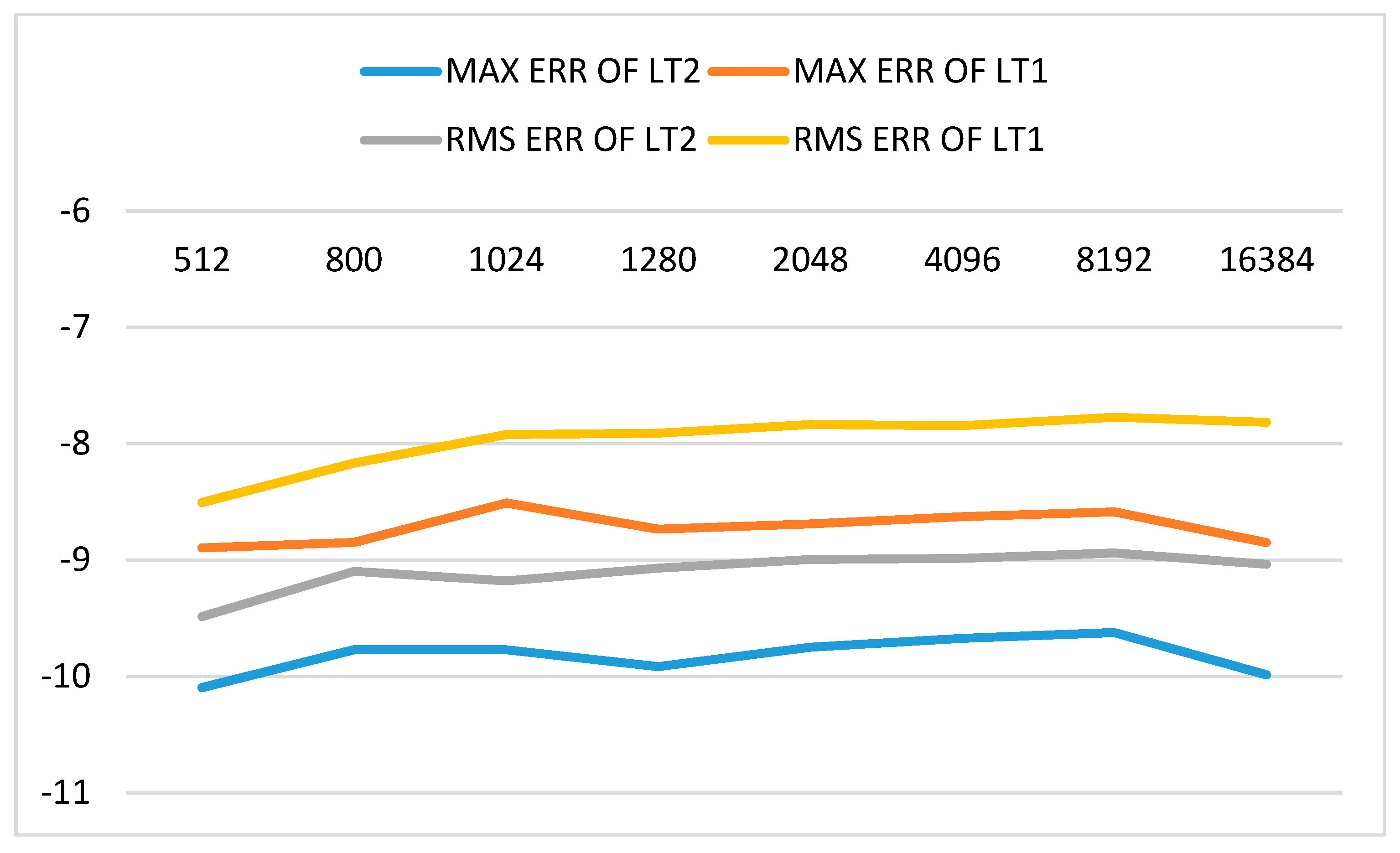
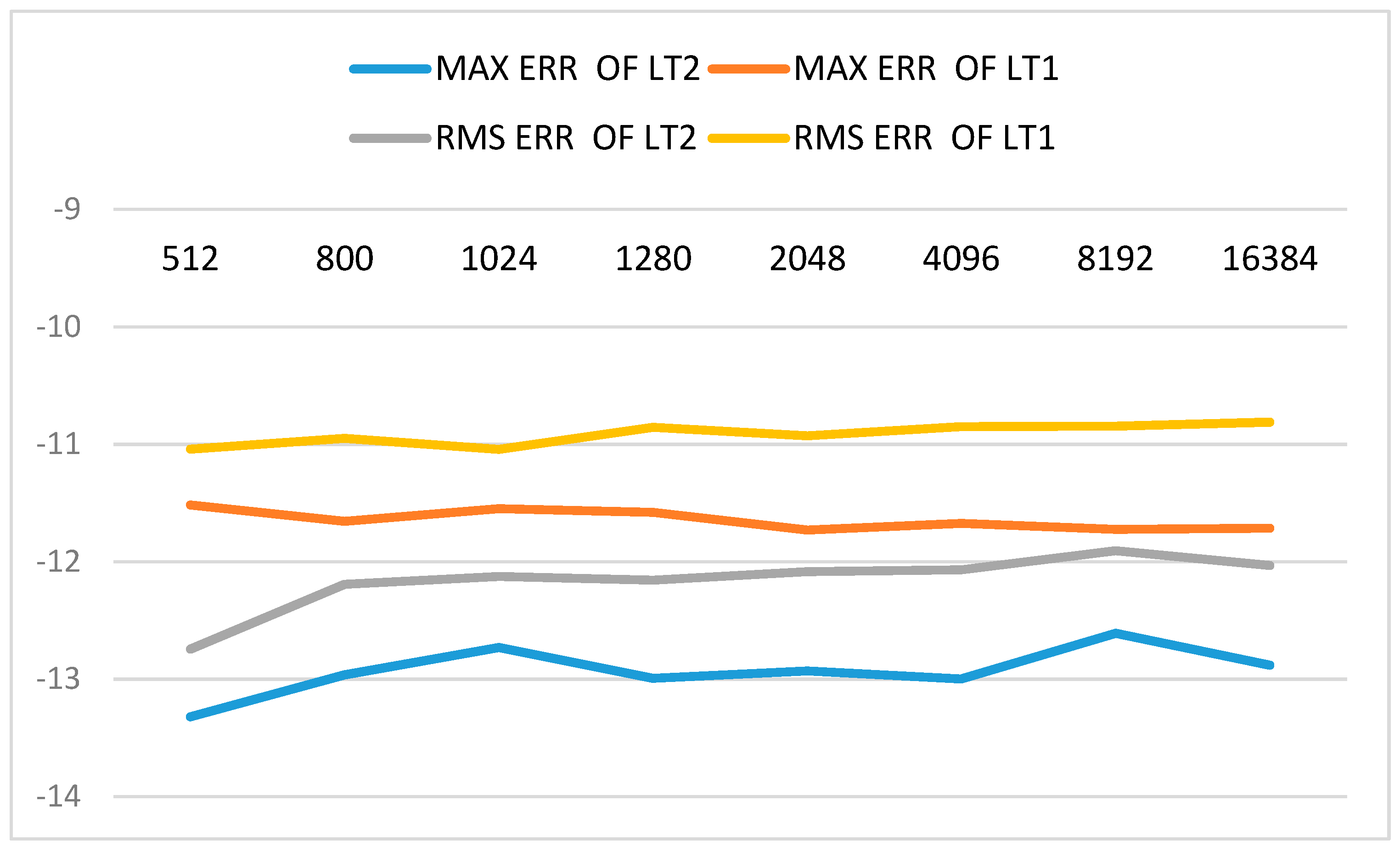
Figure 2, Figure 3 and Figure 4 show the errors of LT with CMAX = 64 in log10 form for EPS = 1.0E-05, EPS = 1.0E-07 and EPS = 1.0E-10, respectively. Abbreviations “MAX ERR” and “RMS ERR” in Figure 2, Figure 3 and Figure 4 denote maximum error and root-mean-square error, respectively. It can be found that both maximum error and root-mean-square error of LT2 are improved by about one order magnitude than LT1. The results show that the proposed method is effective in improving the accuracy of Legendre transform using butterfly algorithm.

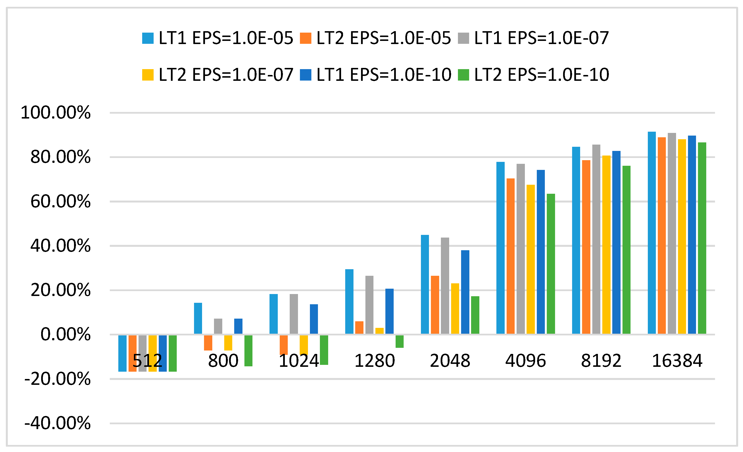
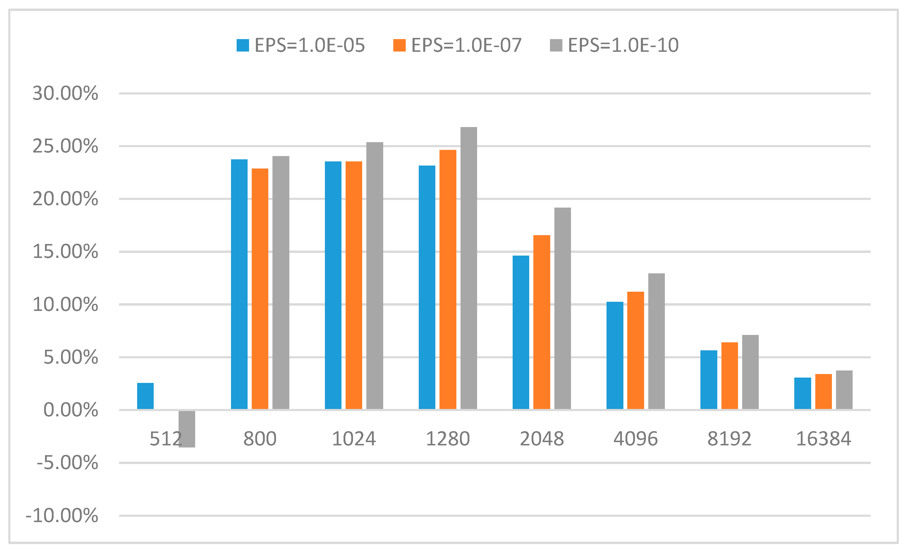
Figure 5 shows the computational time for different Legendre transform algorithms. The speedup and loss speedup of LT2 with CMAX = 64 are demonstrated in Figure 6 and Figure 7, respectively. Loss speedup which measures the relative performance penalty is defined as the speedup of LT1 minus the speedup of LT2 and divided by the speedup of LT0. From Figure 5 and Figure 6, LT2 begins to be faster than LT0 when N = 2048 and achieves more than 26%, 22%, 17% reduction in elapsed time for EPS = 1.0E-5, EPS = 1.0E-7 and EPS = 1.0E-10. LT2 has achieved more than 17%, 63%, 75% and 86% reduction in elapsed time for a run of N2048, N4096, N8192 and N16384, respectively. In Figure 7, the loss speedup of LT2 relative to LT1 is less than 21%, 11%, 7% and 4% for N = 2048, 4096, 8192 and 16,384, respectively. Moreover, the loss speedup of LT2 relative to LT1 decreases rapidly with the increase of N. According to the results of Yin [3], the potential instability of interpolative decomposition only exists in the case of very high order. So, the presented method can alleviate the potential instability of interpolative decomposition at a very small computational burden.

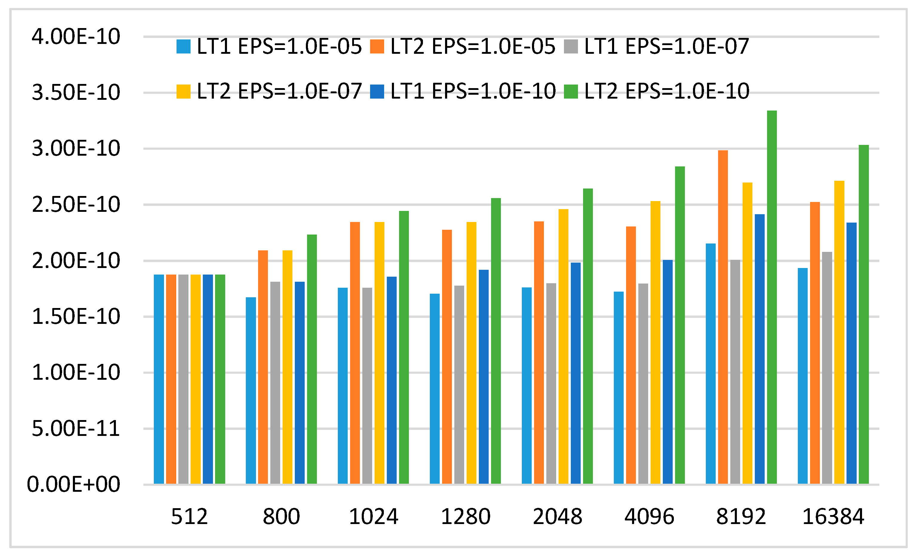
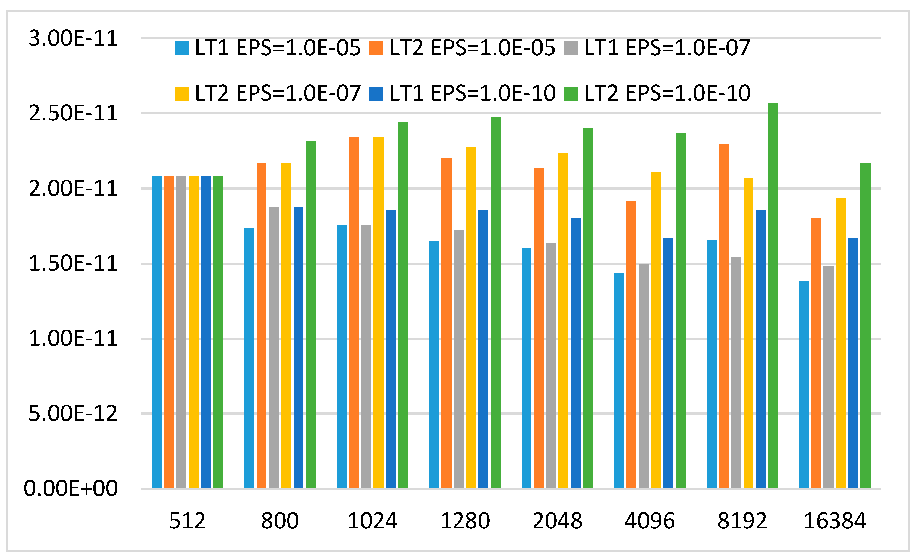
Figure 8 and Figure 9 show the computational time of LT scaled by Nlog³N and Nlog⁴N, respectively. It can be found that the computational complexity of LT2 appears to a little bigger than LT1. The boundary blocks which can’t be accurately expressed by the asymptotic formula and the internal blocks with dimension less that dimensional thresh value result in the increase of the computational complexity. Although the results of LT2 are bigger than those of LT1, LT2 has a similar trend as LT1 in Figure 8 and Figure 9. This means that LT2 has the same computational complexity O(Nlog³N) as LT1.

Legendre-Vandermond matrix is divided into boundary blocks and internal blocks. Boundary blocks which can’t be accurately expressed by the asymptotic formula cause instability of interpolative decompositions and are not suitable for interpolation decomposition. The matrix-vector multiplication based on butterfly algorithm is faster than BLAS function DGEMV only when the dimension of matrix is greater than or equal to 512. Internal blocks with lower matrix dimension adopt direct matrix-vector multiplication instead of butterfly algorithm. The number of nonzero elements of boundary blocks, internal blocks which do not participate in interpolation decomposition cause the increase of the computational cost compare to Tygert’s algorithm. Therefore, through reasonable partitioning, the theoretical computational complexity of the proposed method can reach the optimal computational complexity O(Nlog²N/loglogN).

6. Conclusions

In this paper, a high accurate and stable Legendre transform algorithm is proposed. A block partitioning based on asymptotic formula is employed to mitigate the potential instability of Legendre transform using butterfly algorithm. The Legendre-Vandermonde matrix is divided into one block $P_{\mathrm{N}}^{\mathrm{REC}}\left({\underset{\_}{x}}_N^{leg}\right)$ and $K$ sub-matrices $P_{\mathrm{N}}^{\left(k\right)}\left(x_N^{leg}\right)$. Instead of FFT method, butterfly algorithm is employed to compute $P_{\mathrm{N}}^{\left(k\right)}\left(x_N^{leg}\right){\underset{\_}{c}}_N^{leg}$. Numerical results demonstrate that the proposed method improves stability by about one order magnitude than Tygert’s algorithm (2010), while only sacrifices less than 7% speedup for very high order (N ≥ 4096) Legendre transform.

Although the computational time of proposed method is a little bigger than Tygert’s algorithm, it has the same computational complexity O(Nlog³N) as Tygert’s algorithm. Moreover, the proposed method is equivalent to Tygert’s algorithm when no block partition is used. In the application of NWP, an additional dimensional thresh value could be introduced to include Tygert’s algorithm (2010) for further reducing the computational complexity.

In the future, we will study the more optimal block partition method to improve the computational performance, while still keeping stability and making a detailed analysis in regard to the spectral harmonic transform using the proposed method for very high resolution—especially its performance in the reduction of potential numerical instability for resolution T7999.

References

- Seljebotn, D.S. Wavemoth—Fast spherical harmonic transforms by butterfly matrix compression. Astrophys. J. 2012, 199, 1–12. [Google Scholar] [CrossRef]
- Wedi, N.P.; Hamrud, M.; Mozdzynski, G. A Fast Spherical Harmonics Transform for Global NWP and Climate Models. Mon. Weather Rev. 2013, 141, 3450–3461. [Google Scholar] [CrossRef]
- Yin, F.; Wu, G.; Wu, J.; Zhao, J.; Song, J. Performance evaluation of the fast spherical harmonic transform algorithm in the yin–he global spectral model. Mon. Weather Rev. 2018, 146, 3163–3182. [Google Scholar] [CrossRef]
- Suda, R.; Takami, M. A fast spherical harmonics transform algorithm. Math. Comput. 2002, 71, 703–715. [Google Scholar] [CrossRef]
- Kunis, S.; Potts, D. Fast spherical Fourier algorithms. J. Comput. Appl. Math. 2003, 161, 75–98. [Google Scholar] [CrossRef] [Green Version]
- Suda, R. Stability analysis of the fast Legendre transform algorithm based on the fast multipole method. In Proceedings of the Estonian Academy of Sciences Physics; Tallinn Book Printers Ltd.: Tallinn, Estonia, 2004; Volume 53, pp. 107–115. [Google Scholar]
- Suda, R. Fast Spherical Harmonic Transform Routine FLTSS Applied to the Shallow Water Test Set. Mon. Weather Rev. 2005, 133, 634–648. [Google Scholar] [CrossRef]
- Rokhlin, V.; Tygert, M. Fast Algorithms for Spherical Harmonic Expansions. SIAM J. Sci. Comput. 2005, 27, 1903–1928. [Google Scholar] [CrossRef]
- Tygert, M. Recurrence relations and fast algorithms. Appl. Comput. Harmon. Anal. 2006, 28, 121–128. [Google Scholar] [CrossRef]
- Tygert, M. Fast algorithms for spherical harmonic expansions, II. J. Comput. Phys. 2008, 227, 4260–4279. [Google Scholar] [CrossRef] [Green Version]
- Tygert, M. Short Note: Fast algorithms for spherical harmonic expansions, III. J. Comput. Phys. 2010, 229, 6181–6192. [Google Scholar] [CrossRef]
- Michielssen, E.; Boag, A. A multilevel matrix decomposition algorithm for analyzing scattering from large structures. IEEE Trans. Antenn. Propag. 1996, 44, 1086–1093. [Google Scholar] [CrossRef]
- O’Neil, M.; Woolfe, F.; Rokhlin, V. An algorithm for the rapid evaluation of special function transforms. Appl. Comput. Harmon. Anal. 2010, 28, 203–226. [Google Scholar] [CrossRef] [Green Version]
- Li, Y.; Yang, H. Interpolative Butterfly Factorization. SIAM J. Sci. Comput. 2017, 39, A503–A531. [Google Scholar] [CrossRef] [Green Version]
- Wu, J.P.; Zhao, J.; Song, J.Q.; Zhang, W.M. Preliminary design of dynamic framework for global non-hydrostatic spectral model. Comput. Eng. Des. 2011, 32, 3539–3543. [Google Scholar]
- Yang, J.; Song, J.; Wu, J.; Ren, K.; Leng, H. A high-order vertical discretization method for a semi-implicit mass-based non-hydrostatic kernel. Q. J. R. Meteorol. Soc. 2015, 141, 2880–2885. [Google Scholar] [CrossRef]
- Yang, J.; Song, J.; Wu, J.; Ying, F.; Peng, J.; Leng, H. A semi-implicit deep-atmosphere spectral dynamical kernel using a hydrostatic-pressure coordinate. Q. J. R. Meteorol. Soc. 2017, 143, 2703–2713. [Google Scholar] [CrossRef]
- Cheng, H.; Gimbutas, Z.; Martinsson, P.G.; Rokhlin, V. On the compression of low rank matrices. SIAM J. Sci. Comput. 2005, 26, 1389–1404. [Google Scholar] [CrossRef]
- Heitman, Z.; Bremer, J.; Rokhlin, V. On the existence of nonoscillatory phase functions for second order ordinary differential equations in the high-frequency regime. J. Comput. Phys. 2015, 290, 1–27. [Google Scholar] [CrossRef]
- Bremer, J.; Rokhlin, V. Improved estimates for nonoscillatory phase functions. Discrete Cont. Dyn.-Am. 2016, 36, 4101–4131. [Google Scholar] [CrossRef] [Green Version]
- Bremer, J.; Rokhlin, V. On the nonoscillatory phase function for Legendre’s differential equation. J. Comput. Phys. 2017, 350, 326–342. [Google Scholar] [CrossRef]
- Bremer, J.; Yang, H. Fast algorithms for Jacobi expansions via nonoscillatory phase functions. IMA J. Numer. Anal. 2018, arXiv:1803.03889. [Google Scholar]
- Glaser, A.; Liu, X.; Rokhlin, V. A fast algorithm for the calculation of the roots of special functions. SIAM J. Sci. Comput. 2019, 29, 1420–1438. [Google Scholar] [CrossRef]
- James, B.; Qiyuan, P.; Haizhao, Y. Fast Algorithms for the Multi-dimensional Jacobi Polynomial Transform. arXiv 2019, arXiv:1901.07275. [Google Scholar]
- ButterflyLab. Available online: https://github.com/ButterflyLab/ButterflyLab (accessed on 14 August 2019).
- Candès, E.; Demanet, L.; Ying, L. A Fast Butterfly Algorithm for the Computation of Fourier Integral Operators. Multiscale Model. Simul. 2009, 7, 1727–1750. [Google Scholar] [CrossRef]
- Hale, N.; Townsend, A. A fast, simple, and stable Chebyshev-Legendre transform using an asymptotic formula. SIAM J. Sci. Comput. 2014, 36, 148–167. [Google Scholar] [CrossRef]
- Hale, N.; Townsend, A. A fast FFT-based discrete Legendre transform. IMA J. Numer. Anal. 2015, 36, 1670–1684. [Google Scholar] [CrossRef] [Green Version]
- Townsend, A.; Webby, M.; Olver, S. Fast polynomial transforms based on Toeplitz and Hankel matrices. Math. Comput. 2018, 87, 1913–1934. [Google Scholar] [CrossRef]
- Stieltjes, T.J. Sur les polynômes de Legendre. Ann. Fac. Sci. Toulouse 1890, 4, G1–G17. [Google Scholar] [CrossRef]
- Liao, X.; Xiao, L.; Yang, C.; Lu, Y. MilkyWay-2 supercomputer: System and application. Front. Comput. Sci. 2014, 8, 345–356. [Google Scholar] [CrossRef]
- Martinsson, P.G.; Rokhlin, V.; Shkolnisky, Y.; Tygert, M. ID: a software package for low rank approximation of matrices via interpolative decompositions, version 0.2. Available online: http://cims.nyu.edu/~tygert/id_doc.pdf (accessed on 4 August 2017).
- Mark Tygert’s Homepage. Available online: http://tygert.com/software.html (accessed on 14 August 2019).
Figure 1.
Partitioning of the Legendre-Vandermonde matrix for N = 1024 (in which matrix B is the boundary parts can’t be accurately expressed by the asymptotic formula while matrix P is the internal parts can. There are 2(K + 1) sub-matrices of B and 2K sub-matrices of P. According to the symmetric or anti-symmetric property of Legendre polynomials, we only need to consider K + 1 sub-matrices of B and K sub-matrices of P on top).
Figure 2.
Errors of LT in log10 form with EPS = 1.0E-05 and CMAX = 64 (LT1 is the butterfly algorithm and LT2 is the proposed method. Abbreviations “MAX ERR” and “RMS ERR” denote the maximum error and root-mean-square error, respectively. EPS is desired precision in interpolative decomposition, CMAX is the number of columns in each sub-matrix on level 0).
Figure 3.
Errors of LT in log10 form with EPS = 1.0E-07 and CMAX = 64 (LT1 is the butterfly algorithm and LT2 is the proposed method. Abbreviations “MAX ERR” and “RMS ERR” denote the maximum error and root-mean-square error, respectively. EPS is desired precision in interpolative decomposition, CMAX is the number of columns in each sub-matrix on level 0).
Figure 4.
Errors of LT in log10 form with EPS = 1.0E-10 and CMAX = 64 (LT1 is the butterfly algorithm and LT2 is the proposed method. Abbreviations “MAX ERR” and “RMS ERR” denote the maximum error and root-mean-square error, respectively. EPS is desired precision in interpolative decomposition, CMAX is the number of columns in each sub-matrix on level 0).
Figure 5.
Computational time for different Legendre transform algorithms with CMAX = 64 (LT0 is the algorithm using DGEMM, LT1 is the butterfly algorithm and LT2 is the proposed method, EPS is desired precision in interpolative decomposition, CMAX is the number of columns in each sub-matrix on level 0, Unit: Second).
Figure 6.
Speedup of LT1 and LT2 with CMAX = 64 compare to LT0 (LT0 is the algorithm using DGEMM, LT1 is the butterfly algorithm and LT2 is the proposed method, EPS is desired precision in interpolative decomposition, CMAX is the number of columns in each sub-matrix on level 0).
Figure 7.
Loss speedup of LT2 with CMAX = 64 compare to LT1 (LT1 is the butterfly algorithm and LT2 is the proposed method, EPS is desired precision in interpolative decomposition, CMAX is the number of columns in each sub-matrix on level 0).
Figure 8.
Computational time scaled by Nlog3N with CMAX = 64(LT1 is the butterfly algorithm and LT2 is the proposed method. EPS is desired precision in interpolative decomposition, CMAX is the number of columns in each sub-matrix on level 0).
Figure 9.
Computational time scaled by Nlog4N with CMAX = 64 (LT1 is the butterfly algorithm and LT2 is the proposed method. EPS is desired precision in interpolative decomposition, CMAX is the number of columns in each sub-matrix on level 0).
© 2019 by the authors. Licensee MDPI, Basel, Switzerland. This article is an open access article distributed under the terms and conditions of the Creative Commons Attribution (CC BY) license (http://creativecommons.org/licenses/by/4.0/).
Share and Cite
MDPI and ACS Style
Yin, F.; Wu, J.; Song, J.; Yang, J. A High Accurate and Stable Legendre Transform Based on Block Partitioning and Butterfly Algorithm for NWP. Mathematics 2019, 7, 966. https://doi.org/10.3390/math7100966
AMA Style
Yin F, Wu J, Song J, Yang J. A High Accurate and Stable Legendre Transform Based on Block Partitioning and Butterfly Algorithm for NWP. Mathematics. 2019; 7(10):966. https://doi.org/10.3390/math7100966
Chicago/Turabian StyleYin, Fukang, Jianping Wu, Junqiang Song, and Jinhui Yang. 2019. "A High Accurate and Stable Legendre Transform Based on Block Partitioning and Butterfly Algorithm for NWP" Mathematics 7, no. 10: 966. https://doi.org/10.3390/math7100966
Note that from the first issue of 2016, this journal uses article numbers instead of page numbers. See further details here.