An Intelligent Algorithm for Solving the Efficient Nash Equilibrium of a Single-Leader Multi-Follower Game

Abstract

This aim of this paper is to provide the immune particle swarm optimization (IPSO) algorithm for solving the single-leader–multi-follower game (SLMFG). Through cooperating with the particle swarm optimization (PSO) algorithm and an immune memory mechanism, the IPSO algorithm is designed. Furthermore, we define the efficient Nash equilibrium from the perspective of mathematical economics, which maximizes social welfare and further refines the number of Nash equilibria. In the end, numerical experiments show that the IPSO algorithm has fast convergence speed and high effectiveness.

1. Introduction

In 1950, Nash equilibrium was formulated based on noncooperative games formed among all players, and the existence of an equilibrium point was proven [1,2]. In economics, most noncooperative game theory has focused on equilibrium in games, especially Nash equilibrium and its refinements [3]. Nash equilibrium means that every player cannot obtain additional advantage by adjusting his/her present strategy individually. The Nash equilibrium has played significant roles in many disciplines: psychology, economics, engineering management, computer sciences [4], reinsurance bargaining [5], etc. The Nash equilibrium may not be unique but multiple. Thus, the player is confused when making decisions. For the refinement of the Nash equilibrium, efficiency is introduced by using the efficient mechanism design of mathematical economics [6]. This paper proposes the efficient Nash equilibrium, which can be beneficial to all players in that social welfare is maximized and the number of Nash equilibria is greatly reduced. Hence, the study of the efficient Nash equilibrium has certain practical significance.

A single-leader–multi-follower game (SLMFG) is a special form of the leader–follower game, also called the bilevel programming problem. Yu [7] introduced the Nash equilibrium point existence theorem for the SLMFG and multi-leader–follower game. Jia et al. [8] established the existence theorem for the weakly Pareto Nash equilibrium of the SLMFG. Furthermore, SLMFGs are widely used in resource coordination [9], energy scheduling [10], cellular data traffic and 5G networks [11], hexarotors with tilted propellers [12], etc. The SLMFG contains one leader and multiple followers. The leader is capable of dominating and expecting the responses of the followers, and the leader selects the best strategy from his own feasible strategy space by knowing the responses of the followers. The followers make their optimal responses according to the leader’s given strategy. Currently, many problems can be treated as leader–follower problems in reality, such as those between suppliers and retailers [13], between groups and subsidiaries, between central and local governments [14], and between defenders and multiple attackers [15].

Furthermore, a SLMFG is regarded as a bilevel programming problem with a leader–follower hierarchical structure [16]. Currently, the study of linear bilevel programming is relatively mature, but the studies on nonlinear bilevel programming are lacking. Nonlinear bilevel programming is a NP-hard problem [17,18]. Fortunately, with the development of biological evolution and heuristic algorithms, swarm intelligent algorithms have displayed the potential for possibly solving nonlinear bilevel programming problems. Many scholars have tried to solve the Nash equilibrium of the SLMFG by using swarm intelligence algorithms, including a dynamic particle swarm optimization algorithm [19], genetic algorithms [20,21], and a nested evolutionary algorithm [22]. We consider swarm intelligence algorithms for solving the SLMFG, which has an evident theoretic foundation and applied significance.

The paper is organized as follows. In the next section, we present the model of the single-leader–multi-follower game, the efficient Nash equilibrium of the SLMFG, and some assumptions of the SLMFG. In Section 3, we consider that the SLMFG is turned into a nonlinear equation problem (NEP) by using the Karush–Kuhn–Tucker (KKT) condition and complementarity function methods. In Section 4, the IPSO algorithm consists of introducing the antibody concentration inhibition mechanism and immune memory function into the particle swarm optimization (PSO) algorithm. In Section 5, we solve some numerical experiments by utilizing the IPSO algorithm. Additionally, the IPSO algorithm has the advantages of few parameters, easy implementation, and random generation of the initial point. Furthermore, the IPSO algorithm has a fast convergence speed, as shown by observing its off-line performance. Finally, several numerical experiments showed that the IPSO algorithm is practicable: the efficient Nash equilibrium is solved and the number of Nash equilibria is greatly reduced.

2. Preliminaries and Prerequisites

In this section, we present the model of the SLMFG, the efficient Nash equilibrium, and some assumptions of the SLMFG.

2.1. The Model of the Single-Leader Multi-Follower Game (SLMFG)

Assume that $I=\{1,2,\dots ,n\}$ is a set of followers and $y_i$ ($i\in I$) is the control vector of the ith follower. The ith follower’s feasible strategy set is $Y_i$ ($i\in I$), where $Y={\displaystyle \prod _{i=1}^n}{Y}_i$, $Y_{-i}={\displaystyle \prod _{j\in I\setminus \left\{i\right\}}}{Y}_j$, and $-i=I\setminus \left\{i\right\}$. The leader’s feasible strategy set is X, and $x\in X$ is the control vector of the leader. The objective function of the leader is $\phi :X\times Y\to \mathbb{R}$, and the followers’ objective functions are $f_i:X\times Y\to \mathbb{R}$. Furthermore, the followers’ best response feasible strategies regarding the leader’s strategy parameter x are defined by the set-value mapping $K:X\to 2^Y$ as follows:

$$K\left(x\right)=\{y\in Y|f_i(x,y_i,y_{-i})=\underset{u_i\in Y_i}{min}{f}_i(x,u_i,y_{-i})\}.$$

(1)

Assume that a strategy profile for the followers is $y^{*}=(y_1^{*},y_2^{*},\dots ,y_n^{*})\in Y$; for any $i\in I$, the following equation is satisfied:

$$f_i(x,y_i^{*},y_{-i}^{*})\le f_i(x,u_i,y_{-i}^{*}),u_i\in Y_i.$$

(2)

In that case $y^{*}$ is called the Nash equilibrium of the followers if the leader’s strategy $x^{*}$ satisfies

$$\phi (x^{*},y^{*})=\underset{x\in X}{max}\phi (x,y^{*}).$$

(3)

$x^{*}$ is the Nash equilibrium of the leader; hence, the strategy profile $(x^{*},y^{*})$ is the Nash equilibrium of the SLMFG, and this means that each follower cannot obtain additional payment by altering his/her recent strategy singly, that is, every follower makes his/her best response when the strategy of the leader is given.

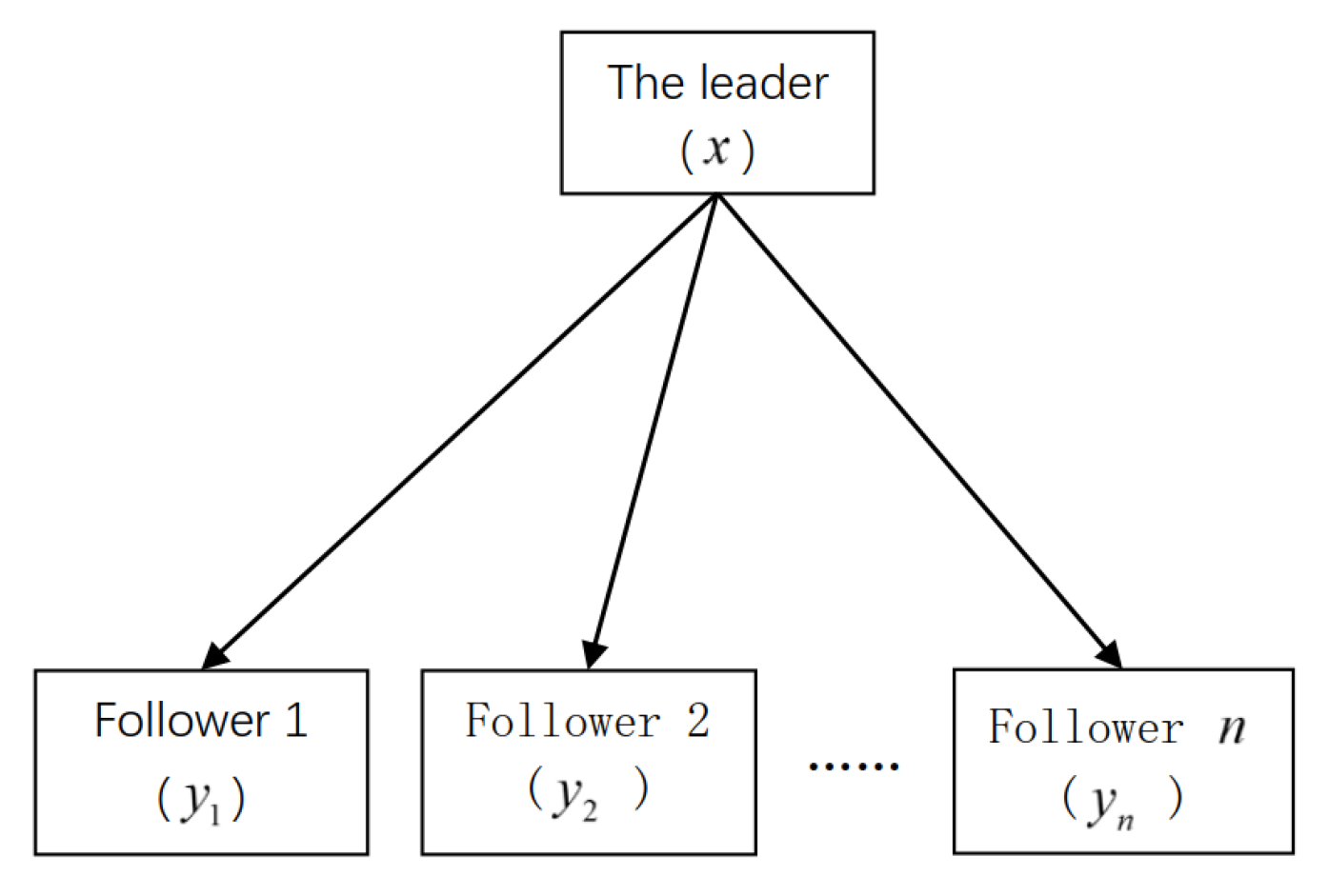
The SLMFG (Figure 1) model of a leader and n followers be expressed as follows:

2.2. The Special Form of the SLMFG

From now on, we make the following some assumptions:

Assumption 1.

(a) 

The leader’s objective function $\phi :X\times Y\to \mathbb{R}$ and the leader’s feasible set G, $G:X\to \mathbb{R}$ are both continuous.

(b) 

The followers’ objective functions $f_i:X\times Y\to \mathbb{R}(i\in I)$ and the followers’ constraint functions $g_i:X\times Y\to \mathbb{R}$ are both differentiable with local Lipschitz continuity.

(c) 

For every follower $i\in I$, given any $y_{-i}$, each follower’s objective function $f_i(x,y_i,y_{-i})(i\in I)$ is convex concerning $y_i$, and the constraint function $g_i(x,y_i,y_{-i})$ is convex with respect to $y_i$.

A general expression for the above model is as follows:

$$\begin{array}{c}\hfill \begin{array}{cc}& \mathrm{The}\mathrm{leader}:\left\{\begin{array}{c}\underset{x\in X}{max}\phi (x,y),\hfill \\ \mathrm{s}.\mathrm{t}.G\left(x\right)\le 0,\hfill \end{array}\right.\hfill \\ & \mathrm{The}\mathrm{followers}:\forall i\in I,\left\{\begin{array}{c}\underset{y\in Y}{min}{f}_i(x,y),\hfill \\ \mathrm{s}.\mathrm{t}.g_i(x,y_i,y_{-i})\le 0,\hfill \end{array}\right.\hfill \end{array}\end{array}$$

(4)

where x and y denote the leader’s decision variable and the followers’ decision variables, respectively. $\phi$ represents the leader’s objective function and $f_i(i\in I)$ represent the followers’ objective functions. The leader first selects his/her own strategy x, and the followers choose their own strategies $y=(y_1,\dots ,y_n)$ through the leader’s given strategy x.

We define the set for problem (4) as follows [18,23]:

The feasible set of problem (4) is $\Omega =\{(x,y)\in X\times Y|G\left(x\right)\le 0,g_i(x,y_i,y_{-i})\le 0\}$. For fixed values of $x\in X$, the feasible set for the followers is $\Omega \left(x\right)=\{y\in Y|g_i(x,y_i,y_{-i})\le 0\}$. The projection of $\Omega$ in the leader’s decision space is represented by $\overline{X}=\left\{x\right|\exists y,\mathrm{s}.\mathrm{t}.(x,y)\in \Omega \}$. For fixed values of $x\in \overline{X}$, the response set for the followers is $K\left(x\right)=\left\{y\right|y\in \mathrm{argmin}\left\{f_i(x,y)\right|y\in \Omega \left(x\right)\}\}$, and the induced domain of problem (4) is $\Xi =\left\{(x,y)\right|x\in \overline{X},y\in K\left(x\right)\}$. Thus, the problem (4) can be translated into an optimization problem as follows:

$$\max \left\{\phi \right(x,y\left)\right|(x,y)\in \Xi \}.$$

(5)

Since the Nash equilibrium may not be unique but multiple, the players are confused when making decisions. The refinement of the Nash equilibrium is an essential prerequisite. Thus, the concept of efficiency is incorporated into the Nash equilibrium, called the efficient Nash equilibrium, which maximizes social welfare and further refines the number of Nash equilibria. Efficient Nash equilibrium expresses a win–win idea under certain conditions, making it beneficial to all players and enabling it to reduce the number of Nash equilibria.

2.3. The Definition of Efficient Nash Equilibrium

We give the following some definitions:

Definition 1

(Efficiency) [6]). If a strategy maximizes social welfare in a way that the leader obtains the biggest rewards and the sum of the followers’ payoff is the smallest in the entire feasible strategy space, then it is called efficient.

Definition 2

(Efficient Nash equilibrium). Let S be all Nash equilibrium strategies of the SLMFG, the sum function mapping is $U:X\times Y\to \mathbb{R}$, $U_k(x,y)(k=0,1,\dots ,n)$ indicates the sum of the payoffs obtained from all Nash equilibrium strategies S, where $k=0$ denotes the payoff sum from the leader’s strategy and $k=1,\dots ,n$ denote the payoff sums from followers’ strategy. If the sum of the payoffs $Z^{*}(Z^{*}\in S)$, then, for any other strategy, the sum of the payoffs $Z(Z\in S)$ satisfies the following:

$$\sum _{i=0}^n{U}_i\left(Z\right)\le \sum _{i=0}^n{U}_i\left(Z^{*}\right),\forall Z\in S,$$

and then $Z^{*}$ is called the efficient Nash equilibrium. This means that social welfare is maximized, and each player cannot obtain additional advantages by altering his/her present strategy individually.

The set of Nash equilibria depends on the leader’s decision variable x and the followers’ decision variables $y=(y_1,\dots ,y_n)$. If x and $y=(y_1,\dots ,y_n)$ satisfy the following equation:

$$\phi \left(x^{*}\right)=\underset{x\in X}{max}\phi \left(x\right)=\underset{x\in X}{max}\underset{y\in K\left(x\right)}{max}\phi (x,y),$$

$$y^{*}\in K\left(x^{*}\right),$$

$$\phi (x^{*},y)\le \phi (x^{*},y^{*}),\forall y\in K\left(x^{*}\right),$$

(6)

$$\sum _{i=1}^n{U}_i(x^{*},y)\le \sum _{i=1}^n{U}_i(x^{*},y^{*}),i=1,\dots ,n.$$

Then, $(x^{*},y^{*})$ is the efficient Nash equilibrium of the SLMFG, and this signifies that the leader obtains the largest rewards; the sum of the followers’ payoffs is the smallest under the strategy profile $(x^{*},y^{*})$; and the leader and the followers cannot obtain additional reward by altering their current strategies unilaterally.

3. The Transformation of the SLMFG

When the upper-level leader’s strategy is given, we need to be able to consider converting the lower-level follower problem into a nonlinear equation problem (NEP). Through the Karush–Kuhn–Tucker (KKT) condition, the SLMFG is converted into a nonlinear complementarity problem (NCP), and the nonlinear complementarity problem is transformed into a NEP through the complementarity function method. Therefore, the SLMFG problem is regarded as a nonlinear optimization problem with a bilayer structure, and the SLMFG problem is solved by using the IPSO algorithm.

3.1. The SLMFG Is Turned into a Nonlinear Equation Problem (NEP)

When the followers satisfy Assumption 1(b,c), the optimal solutions of the followers are represented by the Karush–Kuhn–Tucker (KKT) condition, and the followers can be expressed as NCP through the KKT condition [24]. Therefore, when the leader’s strategy x is given, if $y^{*}$ contains the appropriate constraint condition, after that there is a multiplier ${\lambda }_i^{*}$ such that $(x,y_i^{*},{\lambda }_i^{*})$ satisfies the following KKT system [25]:

$$\begin{array}{c}\hfill \begin{array}{ccc}\hfill {\nabla }_{y_i}L(x,y_i,y_{-i}^{*},{\lambda }_i)& =\hfill & 0\\ \hfill 0\le {\lambda }_i\perp -g_i(x,y_i,y_{-i})& \ge \hfill & 0,\end{array}\end{array}$$

(7)

where $g_i(x,y_i,y_{-i})$ are the constraints of the followers, which depend on the control variables of the leader and the control variables of the followers. The Lagrangian function for the ith follower of system (7) is as follows:

$$L(x,y_i,y_{-i},{\lambda }_i)=f_i(x,y_i,y_{-i})+{\lambda }_i{g}_i(x,y_i,y_{-i}).$$

(8)

Consequently, system (7) is regarded as a first-order necessary condition for the followers. Let the SLMFG further satisfy Assumption 1(c); then, $\forall y_{-i}(i=1,2,\dots ,n)$, formula (5) is turned into a convex optimization problem, and system (7) turns into the SLMFG’s sufficient state. We can obtain the following result:

Theorem 1.

Let the $\mathrm{SLMFG}$ satisfy Assumption 1; if $(x^{*},y^{*},{\lambda }^{*})$ satisfies Equation (6) and system (7), then a strategy profile $(x^{*},y^{*})$ is the efficient Nash equilibrium of the SLMFG.

For $\mathcal{F}:\mathbb{R}\times {\mathbb{R}}^n\to \mathbb{R}$, $\mathcal{F}(x,y)=\mathrm{vec}{\left\{{\nabla }_{y_i}{f}_i(x,y_i,y_{-i})\right\}}_{i=1}^n$, system (7) is equal to the system as follows:

$$\begin{array}{c}\hfill \begin{array}{ccc}\hfill \mathcal{F}(x,y)+\sum _{i=1}^n{\nabla }_{y_i}{g}_i(x,y_i,y_{-i}){\lambda }_i& =\hfill & 0\\ \hfill 0\le {\lambda }_i\perp -g_i(x,y_i,y_{-i})& \ge \hfill & 0.\end{array}\end{array}$$

(9)

System (9) is NCP, thus the followers’ problems of the SLMFG are converted into the NCP for the convex optimization. The Lagrangian function is uncertain differentiable, so the function needs to be smoothed further [24,25,26], but the function only needs a differentiable in this paper. However, through the complementary function, the system (9) is converted into a NEP in this paper.

3.2. The Nonlinear Complementarity Problem (NCP) Is Converted into a Nonlinear Equation Problem (NEP)

A NCP is transformed into a NEP through complementarity function methods. The function $\varphi :{\mathbb{R}}^2\to \mathbb{R}$ is called a complementarity function if and only if $\varphi (E,F)=0\iff E\ge 0,F\ge 0,E·F=0$. The Fisher–Burmeister (FB) function can be written as ${\varphi }_{\mathrm{FB}}(E,F)=E+F-\sqrt{E^2+F^2}$, that is, we obtain the following complementarity function:

$$\mathsf{\Theta }(x,y,\lambda )=\left[\begin{array}{c}L(x,y,\lambda )\\ {\theta }_{\mathrm{FB}}(-g_1(x,y),{\lambda }_1)\\ ⋮\\ {\theta }_{\mathrm{FB}}(-g_i(x,y),{\lambda }_i)\\ ⋮\\ {\theta }_{\mathrm{FB}}(-g_n(x,y)),{\lambda }_n)\end{array}\right],$$

(10)

where $\mathsf{\Theta }(x,y,\lambda )$ is a FB function; then, the solution of Equation (10) is equivalent to $\mathsf{\Theta }(x,y,\lambda )=0$. Consequently, the followers’ problems are transformed into a NEP by the Fisher-Burmeister (FB) complementarity function. Thus, the NCP for the followers is converted to a NEP. For the NEP, the IPSO algorithm is designed to solve the optimal responses $y^{*}$ of the followers and the leader’s optimal strategy $x^{*}$, respectively.

For followers, the fitness function is expressed as follows:

$$\mathbb{F}(x,y)={\parallel \mathsf{\Theta }(x,y,\lambda )\parallel }^2.$$

(11)

Obviously, $\mathbb{F}(x,y)=0\iff \mathsf{\Theta }(x,y,\lambda )=0$, which means solving the value of $\underset{x\in \overline{X},y\in K\left(x\right)}{min}\mathbb{F}(x,y)$ under the leader’s fixed strategy. We obtain the followers’ optimal strategies $y^{*}$ by the IPSO algorithm.

For the leader, the fitness function is as follows:

$$\psi (x,y)=\underset{x\in X}{max}\phi (x,y).$$

(12)

Furthermore, we can obtain the leader’s optimal strategy $x^{*}$ by the IPSO algorithm. For the SLMFG, with $(x^{*},y^{*})$ satisfying Definition 2, the efficient Nash equilibrium $(x^{*},y^{*})$ is solved by using the IPSO algorithm. Finally, we obtain a reasonable, efficient Nash equilibrium solution by a refinement of the Nash equilibrium, which implies benefits to all players.

4. The Design of Immune Particle Swarm Optimization (IPSO) Algorithm

For a nonlinear equation equilibrium problem, the IPSO algorithm is designed by incorporating an immune memory function and an antibody concentration inhibition mechanism into the PSO algorithm. In this section, the IPSO algorithm is designed.

4.1. The Particle Swarm Optimization (PSO) Algorithm

The PSO algorithm was originally derived by Kennedy and Eberhart [27]. The PSO algorithm finds the optimal solution through collaboration and shares information among individuals. In the PSO algorithm, the solution of each optimization problem can be viewed as a “particle” in the search space. In the PSO algorithm with a population size of M and an N-dimensional space, $x_i=(x_{i1},x_{i2},\dots ,x_{iN})$ denotes the position vector of particle i and $v_i=(v_{i1},v_{i2},\dots ,v_{iN})$ represents velocity vector of particle i. According to the optimization model, each particle moves towards its own best current position $p_{best}$ (known as personal best) and towards the globally best particle $g_{best}$ (global best). At step t, the basic velocity and position of particle i are updated using the following equation:

$$v_i^{t+1}=w{v}_i^t+c_1{r}_1(p_{best}-x_i^t)+c_2{r}_2(g_{best}-x_i^t),$$

(13)

$$x_i^{t+1}=x_i^t+v_i^{t+1},(i=1,2,\dots ,M),$$

(14)

where $c_1$ is the cognizant factor and $c_2$ is the communal factor. $r_1$ and $r_2$ are two $N\times N$ diagonal elements uniformly distributed in the section [0,1]. w is the inertia weight and w has an impact on the global and local exploration capabilities of the particle. When w is large, the global exploration ability is strong at the beginning of the process. When w is small, the local exploitation ability is stronger in the search space than when the weight is large. At present, increasing the value of the dynamic inertia weight value causes a linear decrease in the weight strategy, and the calculation formula is as follows [28]:

$$w=w_{\max }-\mathrm{T}\frac{w_{\max }-w_{\min }}{{\mathrm{T}}_{\max }},$$

(15)

where $w_{\max }$ is the maximum inertia weight and $w_{\min }$ is the minimum inertia weight. ${\mathrm{T}}_{\max }$ and $\mathrm{T}$ are the maximum number of iterations and the current number of iterations, respectively.

4.2. The Immune Particle Swarm Optimization (IPSO) Algorithm

The IPSO algorithm is a novel intelligent optimization algorithm [29,30] in view of the immune evolution mechanism and information sharing in biological immune systems. The optimal solution is regarded as an antibody, and the functions of object and the restricting terms are considered antigens. The IPSO algorithm is the combination of a probability concentration selection function and the PSO algorithm. During the process of particle (antibody) population updating, we always hope that highly adaptable particles (antibodies) are left behind. If a particle (antibody) is too concentrated, it is difficult to guarantee the diversity of the particle (antibody), and the algorithm may even fall into a local optimum. Therefore, those particles which have worse fitness but a better evolutionary tendency are maintained through the antibody probability concentration selection formula. Antibody $M+Q$ consists of a nonempty set X, and the distance of the antibody $\mathbb{F}(x,y_i)(i=1,2,\dots ,M+Q)$ is calculated by

$${\rho }_1(x,y_i)=\sum _{j=1}^{M+Q}|\mathbb{F}(x,y_i)-\mathbb{F}(x,y_j)|,j=1,2,\dots ,M+Q,$$

(16)

$${\rho }_2(x_i,y)=\sum _{j=1}^{M+Q}|\psi (x_i,y)-\psi (x_j,y)|,j=1,2,\dots ,M+Q.$$

(17)

We can define the concentration formula of particle i as follows:

$${\mathbb{D}}_1(x,y_i)=\frac{1}{{\rho }_1(x,y_i)}=\frac{1}{{\displaystyle \sum _{j=1}^{M+Q}}|\mathbb{F}(x,y_i)-\mathbb{F}(x,y_j)|},$$

(18)

$${\mathbb{D}}_2(x_i,y)=\frac{1}{{\rho }_2(x_i,y)}=\frac{1}{{\displaystyle \sum _{j=1}^{M+Q}}|\psi (x_i,y)-\psi (x_j,y)|}.$$

(19)

We can attain the probability concentration selection function for the followers as [31]:

$${\mathcal{P}}_1(x,y_i)=\frac{\frac{1}{{\mathbb{D}}_1(x,y_i)}}{{\displaystyle \sum _{i=1}^{M+Q}}\frac{1}{{\mathbb{D}}_1(x,y_i)}}=\frac{{\displaystyle \sum _{j=1}^{M+Q}}|\mathbb{F}(x,y_i)-\mathbb{F}(x,y_j)|}{{\displaystyle \sum _{i=1}^{M+Q}}{\displaystyle \sum _{j=1}^{M+Q}}|\mathbb{F}(x,y_i)-\mathbb{F}(x,y_j)|},$$

(20)

where $y_i(i=1,2,\dots ,M+Q)$ represents the particle position for the followers and $\mathbb{F}(x,y_i)$ denotes the fitness value of the function for the followers.

Similarly, we can also obtain the probability density selection function for the leader as follows:

$${\mathcal{P}}_2(x_i,y)=\frac{\frac{1}{{\mathbb{D}}_2(x_i,y)}}{{\displaystyle \sum _{i=1}^{M+Q}}\frac{1}{{\mathbb{D}}_2(x_i,y)}}=\frac{{\displaystyle \sum _{j=1}^{M+Q}}|\psi (x_i,y)-\psi (x_j,y)|}{{\displaystyle \sum _{i=1}^{M+Q}}{\displaystyle \sum _{j=1}^{M+Q}}|\psi (x_i,y)-\psi (x_j,y)|},$$

(21)

where $x_i(i=1,2,\dots ,M+Q)$ represents the particle position for the leader and $\psi (x_i,y)$ is the fitness value of the function for the leader.

Increasing the new population Q primarily maintains the dynamic equilibrium of the population and takes the role of adjusting population concentration. Specifically, when the evolutionary population exhibits worse diversity and weaker global search ability, the IPSO algorithm allows the population to shift to a region with a better evolutionary tendency.

4.3. Implementation Steps of the IPSO Algorithm

The IPSO algorithm implement steps are as follows:

Step 1:

Initialize the parameters. The maximum number of iterations for the followers is ${\mathrm{T}}_1$ and the maximum number of iterations for the leader is ${\mathrm{T}}_2$. The acceleration constants are $c_1$ and $c_2$, the inertia weight values are $w_{max}$ and $w_{min}$, and the precision is $\epsilon$. The size of the randomly generated population is M, and the initial value $x_0$ is randomly generated according to the feasible domain of the leader.

Step 2:

The IPSO algorithm can obtain the initial population $p_0$ by randomly generating the followers’ initial positions $y_i(i=1,2,\dots ,n)$ and initial velocities $v_{yi}$ with the followers’ set-value mappings.

Step 3:

The $\mathrm{IPSO}$ algorithm is used to calculate each particle’s fitness function value for the followers and find the individual best position $p_{ybest}$ and population best position $g_{ybest}$.

Step 4:

Equation (15) is used to compute the inertia weight w.

Step 5:

Equations (13) and (14) are used to update the velocities and positions of followers particles, respectively; compare the fitness functions of the particles; and retain the population best position in the memory library.

Step 6:

Followers are randomly generated to obtain a new population with size Q.

Step 7:

We select population M from the new population $M+Q$ through the probability concentration selection formulation Equation (20).

Step 8:

We choose particles from the memory library to replace particles with poor fitness, and then the immune system produces a next generation of particles $p_1$. Then, the algorithm continues to update the particle velocities and positions by using Equations (13) and (14).

Step 9:

By calculating the fitness value of particle $y_i$’s current position, $y_i$’s fitness value is compared with $y_{i-1}$’s fitness value. If $\mathbb{F}(x_0,y_i)<\mathbb{F}(x_0,y_{i-1})$, then $y_{i-1}=y_i$; otherwise, $y_i=y_{i-1}$.

Step 10:

Each particle’s fitness function value for the followers is calculated, and the individual best position $p_{ybest}$ and population best position $g_{ybest}$ are found. Hence, we can compare the fitness value of the particle $y_i$ with the fitness value of the global $g_{ybest}$; if $\mathbb{F}(x_0,g_{ybest})<\mathbb{F}(x_0,y_i)$, then $y_i=g_{ybest}$; otherwise, $g_{ybest}=y_i$.

Step 11:

Stopping condition of the followers: Does the maximum number of iterations ${\mathrm{T}}_1$ or the precision $|\mathbb{F}\left(x_{i-1}\right)-\mathbb{F}\left(x_i\right)|<{\epsilon }_1$ satisfy the termination condition? If yes, we output the optimal particle $y^{*}$ (approximate solution of the followers); otherwise, we return to Step 4.

Step 12:

The followers’ optimal particle $y^{*}$ is returned as feedback to the leader.

Step 13:

The $\mathrm{IPSO}$ algorithm is used to calculate each particle’s fitness function value for the leader and find the individual best position $p_{xbest}$ and population best position $g_{xbest}$.

Step 14:

The leader particle’s initial position $x_i$ and initial velocity $v_{xi}$ are randomly generated. For each particle i, Equation (13) is applied for updating the velocity of the particle and Equation (14) is applied to update the position of the particle.

Step 15:

A new population number of size Q is randomly generated.

Step 16:

We choose population M from the new population $M+Q$ through the probability concentration selection formula Equation (21).

Step 17:

From the memory library, we choose particles to replace particles with worse fitness among the population, and the immune system generates a new generation of particles $p_1$. Then, the algorithm continues to update the particle velocities and positions by using Equations (13) and (14).

Step 18:

By calculating and comparing $x_i$’s fitness value with $x_{i-1}$’s fitness value, if $\psi (x_i,y^{*})>\psi (x_{i-1},y^{*})$, then $x_{i-1}=x_i$; otherwise, $x_i=x_{i-1}$.

Step 19:

Each particle’s fitness function value for the leader is calculated, and the individual best position $p_{xbest}$ and population best position $g_{xbest}$ are found. Hence, we can compare the particle $x_i$’s fitness value with the global optimal particle $g_{xbest}$’s fitness value; if $\psi (g_{xbest},y^{*})>\psi (x_i,y^{*})$, then $x_i=g_{xbest}$; otherwise, $g_{xbest}=x_i$.

Step 20:

Stopping condition for the leader: Is the maximum number of iterations ${\mathrm{T}}_2$ achieved or is the precision $|\psi \left(x_{i-1}\right)-\psi \left(x_i\right)|<{\epsilon }_2$? If yes, we output the optimal particle $x^{*}$; otherwise, we return to Step 14.

Step 21:

Finally, if $(x^{*},y^{*})$ satisfies Definition 2, then $(x^{*},y^{*})$ denotes the efficient Nash equilibrium set of the SLMFG.

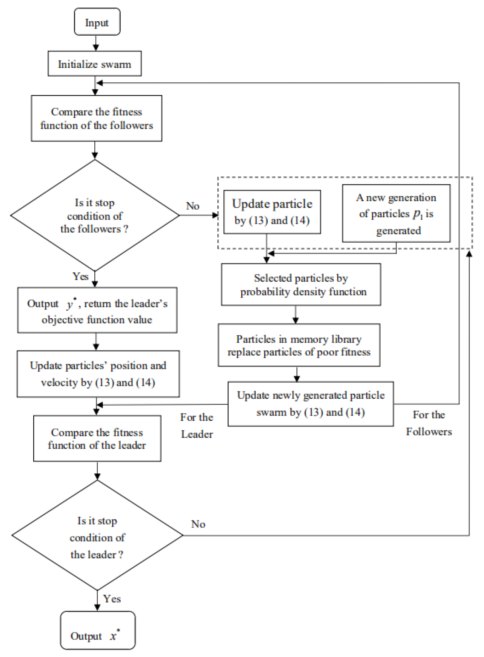
The flow chart of the IPSO algorithm is presented in Figure 2:

4.4. Performance Evaluation of the IPSO Algorithm

The IPSO algorithm expresses a bio-evolving swarm intelligence algorithm that is parallel to genetic algorithms (GAs), such as “natural selection” and “survival of the fittest”. Thus, the measurable analysis method proposed by De Jong [32] can be used for evaluating the convergence of the IPSO algorithm according to its off-line performance.

Definition 3.

The functions off-line performance for the followers and the leader are $s^{*}:\mathbb{R}\to \mathbb{R}$ and $u^{*}:\mathbb{R}\to \mathbb{R}$, respectively. Their final expressions are as follows:

$$\begin{array}{ccc}& & \mathrm{The}\mathrm{followers}:s^{*}(x,y)=\frac{1}{{\mathrm{T}}_1}\sum _{t=1}^{\mathrm{T}}1{\mathbb{F}}^{*}(x,y),\hfill \\ & & \mathrm{The}\mathrm{leader}:u^{*}(x,y)=\frac{1}{{\mathrm{T}}_2}\sum _{t=1}^{\mathrm{T}}2{\psi }^{*}(x,y).\hfill \end{array}$$

From above equations, we know that off-line performance represents the cumulative average of the best fitness function. When particles are closer to the fitness function value, the particles can better adapt to the SLMFG problems, thus the particles are more suitable for the objective functions under certain constraints.

5. Numerical Experiment

The SLMFG can be regarded as a bilevel programming problem. In the paper, the IPSO algorithm is applied for solving the leader’s optimal strategy $x^{*}$ and the followers’ optimal strategy $y^{*}$, respectively. The IPSO algorithm parameters are set as follows: the population size is $M=30$, the learning factors are $c_1=c_2=2$, $w_{\max }=0.2$, and $w_{\min }=0.1$. The maximum numbers for the followers and leader are ${\mathrm{T}}_1=300$ and ${\mathrm{T}}_2=200$, respectively. The size of the new population of followers is $Q=10$ and the precision of the fitness function is set to $\epsilon ={10}^{-3}$. The Nash equilibrium of the SLMFG is solved by the IPSO algorithm, and we can calculate the efficient Nash equilibrium by a refinement of the Nash equilibrium, which implies benefits to all players.

Example 1.

Suppose we have a SLMFG, where the leader strategy is x and the followers’ strategies are $y_1$ and $y_2$. The leader’s payoff function is $\phi (x,y)$, and the followers’ payoff functions are $f_1(x,y_1)$ and $f_2(x,y_2)$.

$$\begin{array}{ccc}& & \underset{x}{max}\phi (x,y)=x{y}_1{y}_2\hfill \\ & & \mathrm{s}.\mathrm{t}.0\le x\le 40.\hfill \\ & & \underset{y_1}{min}{f}_1(x,y_1)={(y_1-4)}^2\hfill \\ & & \mathrm{s}.\mathrm{t}.2y_1+x\le 30,\hfill \\ & & y_1\ge 0.\hfill \\ & & \underset{y_2}{min}{f}_2(x,y_2)={(y_2-5)}^2\hfill \\ & & \mathrm{s}.\mathrm{t}.y_2+2x\le 20,\hfill \\ & & y_2\ge 0.\hfill \end{array}$$

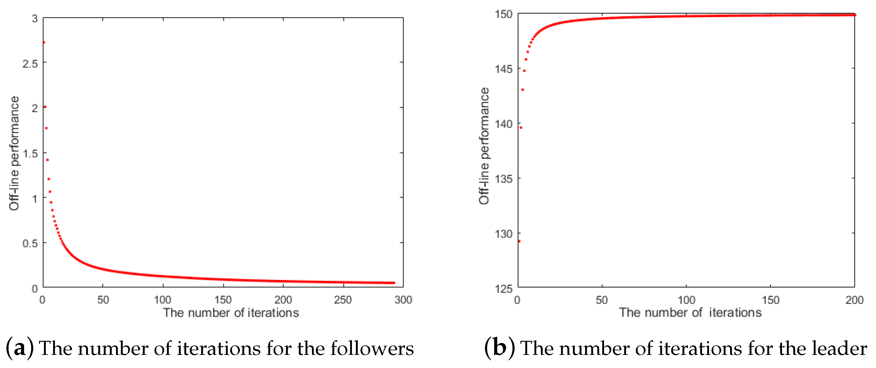
The corresponding numerical results of Example 1 are given in

Table 1. The IPSO algorithm for solving the followers’ result of Example 1.

Times	Number of Iterations	Efficient Nash Equilibrium	Fitness Function Value
1	285	$y_1=3.998$, $y_2=5.026$	21.8 × 10${}^{-3}$
2	274	$y_1=3.998$, $y_2=4.997$	2.2 × 10${}^{-3}$
3	276	$y_1=3.940$, $y_2=5.008$	27.7 × 10${}^{-3}$
4	292	$y_1=3.975$, $y_2=5.043$	44.6 × 10${}^{-3}$
5	288	$y_1=4.031$, $y_2=4.994$	27.9 × 10${}^{-3}$

and

Table 2. The IPSO algorithm for solving the leader’s result of Example 1.

Times	Number of Iterations	Efficient Nash Equilibrium	Fitness Function Value
1	75	$x=7.487$	150.445
2	80	$x=7.501$	149.932
3	84	$x=7.500$	150.000
4	101	$x=7.479$	149.898
5	150	$x=7.5032$	151.022

, and its off-line performance is shown in Figure 3a,b, respectively.

In Table 1, the average number of iterations for the follower problem is 283, and we can obtain that the approximate solution for the followers is ${(4,5)}^{\mathrm{T}}$. In Table 2, the average number of iterations for the leader problem is 98, and we obtain that the leader’s approximate efficient Nash equilibrium is $7.5$. The efficient Nash equilibrium can minimize the income gap for the followers and maximize the rewards earned by the leader, thus strategy $(7.5,4,5)$ is an efficient Nash equilibrium since Example 1 is just unique Nash equilibria. During the calculation process, the number of iterations is small and the convergence of the IPSO algorithm does not depend on the selection of the initial points. Furthermore, it greatly reduces the calculation time of the algorithm, and it does not easily fall into the local optimal solutions. As shown in Figure 3a,b, the off-line performance of the algorithm indicates that the algorithm has a fast convergence speed and is effective.

Example 2.

Suppose we have a SLMFG [33], where the leader strategy is $x=(x_1,x_2,x_3,x_4)$ and the strategies of the followers are $y_1=(y_{11},y_{12})$ and $y_2=(y_{21},y_{22})$. The leader’s payoff function is $\phi (x,y_1,y_2)$, and the followers’ payoff functions are $f_1\left(y_1\right)$ and $f_2\left(y_2\right)$.

$$\begin{array}{ccc}& & \underset{x}{max}\phi (x,y_1,y_2)=(200-y_{11}-y_{21})(y_{11}+y_{21})+(160-y_{12}-y_{22})(y_{12}+y_{22})\hfill \\ & & \mathrm{s}.\mathrm{t}.x_1+x_2+x_3+x_4\le 40,\hfill \\ & & 0\le x_1\le 10,0\le x_2\le 5,0\le x_3\le 15,0\le x_4\le 20.\hfill \\ & & \underset{y_1}{min}{f}_1\left(y_1\right)={(y_{11}-4)}^2+{(y_{12}-13)}^2\hfill \\ & & \mathrm{s}.\mathrm{t}.0.4y_{11}+0.7y_{12}\le x_1,\hfill \\ & & 0.6y_{11}+0.3y_{12}\le x_2,\hfill \\ & & 0\le y_{11},y_{12}\le 20.\hfill \\ & & \underset{y_2}{min}{f}_2\left(y_2\right)={(y_{21}-35)}^2+{(y_{22}-2)}^2\hfill \\ & & \mathrm{s}.\mathrm{t}.0.4y_{21}+0.7y_{22}\le x_3,\hfill \\ & & 0.6y_{21}+0.3y_{22}\le x_4,\hfill \\ & & 0\le y_{21},y_{22}\le 40.\hfill \end{array}$$

For the leader’s decision vector $x_0$, the followers’ corresponding strategy is $(y_1,y_2)$. The optimal decision vector for the followers may not be unique when the strategy of the leader fixed. Thus, the efficient Nash equilibrium is also not unique and may even be multiple, but the number of Nash equilibria is greatly reduced, thus the Nash equilibria are refined efficiently. The followers’ strategy $y=(y_1,y_2)$ is solved by the IPSO algorithm, and the leader’s strategy $x^{*}$ is solved by the IPSO algorithm. The numerical results are shown in

Table 3. The IPSO algorithm for solving the numerical result of Example 2.

x	${\mathit{y}}_1$	${\mathit{y}}_2$	$max\mathit{\phi }(\mathit{x},{\mathit{y}}_1,{\mathit{y}}_2)$	$min{\mathit{f}}_1\left({\mathit{y}}_1\right)$	$min{\mathit{f}}_2\left({\mathit{y}}_2\right)$
(7, 3, 12, 18)	(0, 10)	(30, 0)	6600	25	29
(6.97, 3.03, 12.03, 17.97)	(0.1, 9.9)	(29.9, 0.1)	6600	24.82	29.62
(6.96, 3.04, 12.05, 17.95)	(0.15, 9.85)	(29.85, 0.15)	6600	24.745	29.945
(6.94, 3.06, 12.06, 17.94)	(0.2, 9.8)	(29.8, 0.2)	6600	24.68	30.28
(6.91, 3.09, 12.09, 17.91)	(0.3, 9.7)	(29.7, 0.3)	6600	24.58	30.98
(6.85, 3.15, 12.15, 17.85)	(0.5, 9.5)	(29.5, 0.5)	6600	24.5	32.50
(6.7, 3.3, 12.3, 17.7)	(1, 9)	(29, 1)	6600	25	37
(7.05, 3.13, 11.93, 17.89)	(0.26, 9.92)	(29.82, 0.00)	6599.99	23.47	30.83
⋯	⋯	⋯	⋯	⋯	⋯

:

A run of the IPSO algorithm with 178 iterations for the followers and 105 iterations for the leader was executed. The calculation results are shown in Table 3. When the leader has the greatest benefit, there is dynamic competition among followers, that is, when one player’s income grows, the other player’s income is reduced. The total CPU time spent was 41 s. By Definitions 1 and 2, the leader chooses the strategy that maximizes the total rewards and minimizes followers’ income gap, which means social welfare is maximized, and further each player cannot obtain additional rewards by varying his/her present strategy individually. In Table 3, the minimum total payoff $min\{min{f}_1\left(y_1\right)+min{f}_2\left(y_2\right)\}$ is equal to 54 for the followers, and the smallest income gap $min\{min{f}_1\left(y_1\right)-min{f}_2\left(y_2\right)\}$ is equal to 4. At this point, we can obtain that the efficient Nash equilibrium solution is $(7,3,12,18;0,10;30,0)$ with the leader’s objective value $\phi (x^{*},y^{*})=6600$, and the objective values of the two followers are $f_1\left(y_1^{*}\right)=25$ and $f_2\left(y_2^{*}\right)=29$, respectively. In [21], a run of the genetic algorithm with 600 generations shows that a Stacklberg–Nash equilibrium is $(7.05,3.13,11.93,17.89;0.26,9.92;29.82,0.00)$ with an objective value $\phi (x^{*},y^{*})=6599.99$, and the objective values of two followers are $f_1\left(y_1^{*}\right)=23.47$ and $f_2\left(y_2^{*}\right)=30.83$, which means the smallest income up for the two followers’ is 7.36 and the minimize total payoff is 54.30. As there is a greater income gap between followers and more total payoff than in this paper, the results in [21] are inferior to the IPSO algorithm. In [33], the value of the leader’s objective function is also 6600, but this traditional mathematical analysis method has high computational complexity; the minimum total payoff is 119.42, the smallest income gap is 19.8, and the efficiency is inferior to that of the IPSO algorithm. The IPSO algorithm has a fast convergence speed, saves time, and is effective. In summary, the IPSO algorithm obtains the optimal efficient Nash equilibrium of $(7,3,12,18;0,10;30,0)$, which minimizes the income gap among all followers and maximizes the incomes of the leader.

Example 3.

Suppose we have a SLMFG, where the leader’s strategy is $x=(x_1,x_2,x_3)$ and the strategies of the followers are $y_1=(y_{11},y_{12})$, $y_2=(y_{21},y_{22})$ and $y_3=(y_{31},y_{32})$. The leader’s payoff function is $\phi (x,y_1,y_2,y_3)$, and the follower’s payoff functions are $f_1\left(y_1\right)$, $f_2\left(y_2\right)$ and $f_3\left(y_3\right)$.

$$\begin{array}{ccc}& & \underset{x}{max}\phi (x,y_1,y_2,y_3)=y_{11}{y}_{12}sin{x}_1+y_{21}{y}_{22}sin{x}_2+y_{31}{y}_{32}sin{x}_3\hfill \\ & & \mathrm{s}.\mathrm{t}.x_1+x_2+x_3\le 10,\hfill \\ & & x_1\ge 0,x_2\ge 0,x_3\ge 0.\hfill \\ & & \underset{y_1}{max}{f}_1\left(y_1\right)=y_{11}sin{y}_{12}+y_{12}sin{y}_{11}\hfill \\ & & \mathrm{s}.\mathrm{t}.y_{11}+y_{12}\le x_1,\hfill \\ & & y_{11}\ge 0,y_{12}\ge 0.\hfill \\ & & \underset{y_2}{max}{f}_2\left(y_2\right)=y_{21}sin{y}_{22}+y_{22}sin{y}_{21}\hfill \\ & & \mathrm{s}.\mathrm{t}.y_{21}+y_{22}\le x_2,\hfill \\ & & y_{21}\ge 0,y_{22}\ge 0.\hfill \\ & & \underset{y_3}{max}{f}_3\left(y_3\right)=y_{31}sin{y}_{32}+y_{32}sin{y}_{31}\hfill \\ & & \mathrm{s}.\mathrm{t}.y_{31}+y_{32}\le x_3,\hfill \\ & & y_{31}\ge 0,y_{32}\ge 0.\hfill \end{array}$$

For the optimization problem of the SLMFG, the followers’ strategy is $y=(y_1,y_2,y_3)$ and the leader’s strategy is x. We use the IPSO algorithm to search the optimal solutions. A run of the IPSO algorithm with 254 iterations for the followers and 132 iterations for the leader was executed. The computation results are shown in

Table 4. The IPSO algorithm for solving the numerical result of Example 3.

x	${\mathit{y}}_1$	${\mathit{y}}_2$	${\mathit{y}}_3$	$max\mathit{\phi }(\mathit{x},{\mathit{y}}_1,{\mathit{y}}_2,{\mathit{y}}_3)$	$max{\mathit{f}}_1\left({\mathit{y}}_1\right)$	$max{\mathit{f}}_2\left({\mathit{y}}_2\right)$	$max{\mathit{f}}_3\left({\mathit{y}}_3\right)$
(1.946, 8.054, 0.000)	(0.973, 0.973)	(1.317, 6.737)	(0.000, 0.000)	9.577	1.609	7.099	0.000
(8.054, 1.946, 0.000)	(1.316, 6.738)	(0.973, 0.973)	(0.000, 0.000)	9.577	7.099	1.609	0.000
(0.000, 1.946, 8.054)	(0.000, 0.000)	(0.973, 0.973)	(6.319, 6.735)	9.587	0.000	1.609	7.098
(0.000, 8.054, 1.946)	(0.000, 0.000)	(1.320, 6.734)	(0.973, 0.973)	9.593	0.000	7.098	1.609
(1.946, 0.000, 8.054)	(0.973, 0.973)	(0.000, 0.000)	(1.320, 6.734)	9.593	1.609	0.000	7.098
(8.054, 1.946, 0.000)	(6.734, 1.320)	(0.973, 0.973)	(0.000, 0.000)	9.593	7.098	1.609	0.000
(1.946, 8.054, 0.000)	(0.973, 0.973)	(1.314, 6.378)	(0.000, 0.000)	9.558	1.609	7.094	0.000
⋯	⋯	⋯	⋯	⋯	⋯	⋯	⋯

.

The followers’ strategy $y^{*}=(y_1^{*},y_2^{*},y_3^{*})$ is solved by the IPSO algorithm. $y_1^{*}$, $y_2^{*}$, and $y_3^{*}$ are three identical objective function because their components are equivalent. The leader’s strategy $x^{*}$ is solved by the IPSO algorithm. In Table 4, the efficient Nash equilibrium sets are:

• (0.000, 8.054, 1.946; 0.000, 0.000; 1.320, 6.734; 0.973, 0.973);
• (1.946, 0.000, 8.054; 0.973, 0.973; 0.000, 0.000; 1.320, 6.734); and
• (8.054, 1.946, 0.000; 6.734, 1.320; 0.973, 0.973; 0.000, 0.000).

The efficient Nash equilibrium solution of Example 3 is multiple. By Definitions 1 and 2, to increase efficiency, each player chooses the strategy that minimizes the income gap among the followers and maximizes the total payoffs of the leader. Furthermore, the leader’s objective value is 9.593, the followers’ objective values are one of $\{1.609,7.094,0.000\}$, and $max{\displaystyle \sum _{i=1}^3}{f}_i\left(y_i\right)=18.300$. Thus, when Example 3 obtains the efficient Nash equilibrium, the leader’s maximum benefit is 9.593, and the followers’ total maximum benefit is 18.300. The convergence speed of the IPSO algorithm is superior to that of the algorithm in [21] with 300 generations. The calculation time of the IPSO algorithm is less than that in [34]. The IPSO algorithm has a fast convergence speed, saves more time, and is effective. In Example 3, the IPSO algorithm obtains the optimal efficient Nash equilibrium, which is also the efficient Nash equilibrium set, thereby minimizing the income gap among all followers and maximizing the reward of the leader.

6. Conclusions

This paper considers a single-leader–multi-follower game with a bilevel hierarchical structure. We define the efficient Nash equilibrium by refining of the traditional Nash equilibrium with efficiency; this efficient Nash equilibrium is beneficial to all followers and greatly reduces the number of Nash equilibria, which means social welfare maximization. Furthermore, the SLMFG is transformed into a nonlinear equation problem (NEP) through the the Karush–Kuhn–Tucker (KKT) condition and complementarity function methods. Furthermore, the IPSO algorithm is designed by combining the probability concentration selection function and the PSO algorithm. In conclusion, it can be seen from the comparisons and analyses of the numerical experiments that the IPSO algorithm is effective for solving the efficient Nash equilibrium of a SLMFG. The IPSO algorithm is not dependant on the selection of the initial point, maintains the diversity of the population, and further has the great advantages of global convergence and fast convergence speed. In brief, we provide a swarm intelligence algorithm to solve the bilevel leader–follower game and obtain the efficient Nash equilibrium solution by a refinement of the Nash equilibrium. Solving the multi-leader–multi-follower game by using swarm intelligence algorithms warrants further consideration.

References

- Nash, J. Non-cooperative games. Ann. Math. 1951, 54, 286–295. [Google Scholar] [CrossRef]
- Nash, J. Equilibrium points in n-person games. Proc. Natl. Acad. Sci. USA 1950, 36, 48–49. [Google Scholar] [CrossRef] [PubMed] [Green Version]
- Takako, F.-G. Non-Cooperative Game Theory; Springer: Cham, Switzerland, 2015. [Google Scholar]
- Bhatti, B.A.; Broadwater, R. Distributed Nash equilibrium seeking for a dynamic micro-grid energy trading game with non-quadratic payoffs. Energy 2020, 117709. [Google Scholar] [CrossRef]
- Anthropelos, M.; Boonen, T.J. Nash equilibria in optimal reinsurance bargaining. Insur. Math. Econ. 2020, 93, 196–205. [Google Scholar] [CrossRef]
- Campbell, D.E. Incentives: Motivation and the Economics of Information, 2nd ed.; Cambridge University Press: Cambridge, UK, 2006. [Google Scholar]
- Yu, J.; Wang, H.L. An existence theorem for equilibrium points for multi-leader-follower games. Nonlinear TMA 2008, 69, 1775–1777. [Google Scholar] [CrossRef]
- Jia, W.S.; Xiang, S.W.; He, J.H.; Yang, Y. Existence and stability of weakly Pareto-Nash equilibrium for generalized multiobjective multi-leader-follower games. J. Glob. Optim. 2015, 61, 397–405. [Google Scholar] [CrossRef]
- Bucarey, L.V.; Casorrán, L.M.; Labbé, M.; Ordoñez, F.; Figueroa, O. Coordinating resources in Stackelberg security games. Eur. J. Oper. Res. 2019, 11, 1–13. [Google Scholar] [CrossRef] [Green Version]
- Luo, X.; Liu, Y.F.; Liu, J.P.; Liu, X. Energy scheduling for a three-level integrated energy system based on energy hub models: A hierarchical Stackelberg game approach. Sustain. Cities Soc. 2020, 52, 101814. [Google Scholar] [CrossRef]
- Anbalagan, S.; Kumar, D.; Raja, G.; Balaji, A. SDN assisted Stackelberg game model for LTE-WiFi offloading in 5G networks. Digit. Commun. Netw. 2019, 5, 268–275. [Google Scholar] [CrossRef]
- Lee, M.L.; Nguyen, N.P.; Moonc, J. Leader-follower decentralized optimal control for large population hexarotors with tilted propellers: A Stackelberg game approach. J. Frankl. Inst. 2019, 356, 6175–6207. [Google Scholar] [CrossRef]
- Saberi, Z.; Saberi, M.; Hussain, O.; Chang, E. Stackelberg model based game theory approach for assortment andselling price planning for small scale online retailers. Future Gener. Comput. Syst. 2019, 100, 1088–1102. [Google Scholar] [CrossRef]
- Clempner, J.B.; Poznyak, A.S. Solving transfer pricing involving collaborative and non-cooperative equilibria in Nash and Stackelberg games: Centralized-Decentralized decision making. Comput. Econ. 2019, 54, 477–505. [Google Scholar] [CrossRef]
- Jie, Y.M.; Choo, K.K.R.; Li, M.C.; Chen, L.; Guo, C. Tradeoff gain and loss optimization against man-in-the-middle attacks based on game theoretic model. Future Gener. Comput. Syst. 2019, 101, 169–179. [Google Scholar] [CrossRef]
- Bard, J.F. Practical Bilevel Optimization: Algorithms and Applications; Kluwer Academic Publishers: Dordrecht, The Netherlands, 1998; pp. 193–386. [Google Scholar]
- Jeroslow, R.G. The polynomial hierarchy and a simple model for competitive analysis. Math. Program. 1985, 32, 146–164. [Google Scholar] [CrossRef]
- Gumus, Z.H.; Floudas, C.A. Global optimization of nonlinear bilevel programming problems. J. Glob. Optim. 2001, 20, 1–31. [Google Scholar] [CrossRef]
- Tutuko, B.; Nurmaini, S.; Sahayu, P. Optimal route driving for leader-follower using dynamic particle swarm optimization. In Proceedings of the 2018 International Conference on Electrical Engineering and Computer Science(ICECOS), Pangkal Pinang, Indonesia, 2–4 October 2018; pp. 45–49. [Google Scholar]
- Khanduzi, R.; Maleki, H.R. A novel bilevel model and solution algorithms for multi-period interdiction problem with fortification. Appl. Intell. 2018, 48, 2770–2791. [Google Scholar] [CrossRef]
- Liu, B.D. Stackelberg-Nash equilibrium for multilevel programming with multiple follows using genetic algorithms. Comput. Math. Appl. 1998, 36, 79–89. [Google Scholar] [CrossRef] [Green Version]
- Mahmoodi, A. Stackelberg-Nash equilibrium of pricing and inventory decisions in duopoly supply chains using a nested evolutionary algorithm. Appl. Soft Comput. J. 2020, 86, 105922. [Google Scholar] [CrossRef]
- Amouzegar, M.A. A global optimization method for nonlinear bilevel programming problems. Syst. Man Cybern. 1999, 29, 771–777. [Google Scholar] [CrossRef]
- Facchinei, F.; Fisher, A.; Piccialli, V. Generalized Nash equilibrium problems and Newton methods. Math. Program. 2009, 117, 163–194. [Google Scholar] [CrossRef]
- Li, Q. A Smoothing Newton Method for Generalized Nash Equilibrium Problems; Dalian University of Technology: Dalian, China, 2009. [Google Scholar]
- Izmailov, A.F.; Solodov, M.V. On error bounds and Newton-type methods for generalized Nash equilibrium problems. Comput. Optim. Appl. 2014, 59, 201–218. [Google Scholar] [CrossRef] [Green Version]
- Kennedy, J.; Eberhart, R.C. Particle swarm optimization. In Proceedings of the International Conference on Networks, Singapore, 27–30 August 2002; pp. 1942–1948. [Google Scholar]
- Shi, Y.; Eberhart, R.C. A modified particle swarm optimizer. In Proceedings of the IEEE International Conference on Evolutionary Computation, Anchorage, AK, USA, 4–9 May 1998; pp. 69–73. [Google Scholar]
- Jiao, W.; Cheng, W.; Zhang, M.; Song, T. A simple and effective immune particle swarm optimization algorithm. In Advances in Swarm Intelligence; Springer: Berlin/Heidelberg, Germany, 2012. [Google Scholar]
- Jiang, J.; Song, C.; Ping, H.; Zhang, C. Convergence analysis of self-adaptive immune particle swarm optimization algorithm. In Advances in Neural Networks-ISNN 2018; Lecture Notes in Computer Science; Huang, T., Lv, J., Sun, C., Tuzikov, A., Eds.; Springer: Cham, Switzerland, 2018; Volume 10878. [Google Scholar]
- Lu, G.; Tan, D.; Zhao, M. Improvement on regulating definition of antibody density of immune algorithm. In Proceedings of the International Conference on Neural Information Processing, Singapore, 18–22 November 2002; pp. 2669–2672. [Google Scholar]
- De Jong, K.A. Analysis of the Behavior of a Class of Genetic Adaptive System; University of Michigan: Ann Arbor, MI, USA, 1975. [Google Scholar]
- Bard, J.F. Convex two-level optimization. Math. Program. 1988, 40, 15–27. [Google Scholar] [CrossRef]
- Li, H.; Wang, Y.P.; Jian, Y.C. A new genetic algorithm for nonlinear bilevel programming problem and its global convergence. Syst. Eng. Theory Pract. 2005, 3, 62–71. [Google Scholar]