U.S. Equity Mean-Reversion Examined

Johns Hopkins Carey Business School 100 International Drive, Office 1355, Baltimore, Maryland, 21202, USA
*
Author to whom correspondence should be addressed.
Risks 2013, 1(3), 162-175; https://doi.org/10.3390/risks1030162
Submission received: 16 October 2013
/
Revised: 13 November 2013
/
Accepted: 18 November 2013
/
Published: 4 December 2013
(This article belongs to the Special Issue Risk Factors and Portfolio Choice in the Context of Hedge Fund Investing)
Abstract
:In this paper we introduce an intra-sector dynamic trading strategy that captures mean-reversion opportunities across liquid U.S. stocks. Our strategy combines the Avellaneda and Lee methodology (AL; Quant. Financ. 2010, 10, 761–782) within the Black and Litterman framework (BL; J. Fixed Income, 1991, 1, 7–18; Financ. Anal. J. 1992, 48, 28–43). In particular, we incorporate the s-scores and the conditional mean returns from the Orstein and Ulhembeck (Phys. Rev. 1930, 36, 823–841) process into BL. We find that our combined strategy ALBL has generated a 45% increase in Sharpe Ratio when compared to the uncombined AL strategy over the period from January 2, 2001 to May 27, 2010. These new indices, built to capture dynamic trading strategies, will definitely be an interesting addition to the growing hedge fund index offerings. This paper introduces our first “focused-core” strategy, namely, U.S. Equity Mean-Reversion.
1. Background
Recently, we have seen a proliferation of hedge fund replication products. Often these products are marketed as low cost vehicles for institutional investors to gain broad hedge fund exposure. The case for a cost-effective alternative to direct hedge fund investments becomes very compelling once “fees” and “skills” are taken into consideration.
Fama and French (2010) [4] have shown that active mutual fund managers have difficulty in beating their benchmarks. They document that less than 3% of managers in their sample had statistically significant skill net of fees over the following period of time: January 1984 to September 2006. Whether they employ Fama and French’s (1993) [3] three-factor model or Carhart’s (1997) [5] four-factor model, less than 3% of their sample of 3,156 funds had t-statistics above 2.0. In other words, less than 3% of actively managed mutual funds net of fees exhibit statistically significant skill.
If the result of Fama and French [4] extends to hedge fund managers, that is, if a very small majority of hedge fund managers have statistically significant skills over a long period of time, and products can be created to capture the basic return generating process of these managers, then such products should change our industry. The changes will be fee compression and increased investment process transparency.
For example, suppose that statistical arbitrage (stat arb) managers, in general, do well whenever we are in the state-of-nature where the cross-section of stocks exhibits strong mean-reversion tendencies, i.e., choppy-markets. In such choppy-markets suppose most stat arb managers do well and in non-choppy-markets or strongly trending markets suppose most perform poorly. A benchmark built extract mean-reversion should perform similarly, i.e., generate good returns in choppy-markets and poor returns in non-choppy-markets. Such a benchmark, if constructed properly, should be difficult for approximately 50% of the stat arb managers (gross of fees) to beat. In choppy markets, 50% of the stat arb managers should beat it and 50% should be beaten by it; and in trending market 50% of managers should beat it and 50% should be beaten by it. If one further assumes no manager has skill, the composition of the managers within the top 50% will change over time. If a very small group of managers had skill, then they would consistently beat this benchmark in both choppy and trending market environments.
Let us consider fees, assuming such a benchmark product charges investors 1% management fee and all the stat arb funds charge 2% management fee and 20% incentive fees, then the net of fees performance analysis should favor the benchmark over the managers. A cost-effective investable benchmark product should thus gain traction and ultimately market share from those managers who cannot consistently beat it, which we hypothesize, could be the majority of managers.
Unfortunately, a similar empirical study on hedge fund performance is nearly impossible due to the voluntary nature of hedge fund performance disclosure. We are left to debate this topic without hard empirical supporting or conflicting evidence. Some argue that hedge funds’ return generating processes are too complex to engineer. Hedge fund managers are somehow gifted with this innate ability and this ability cannot be transferred, taught, or duplicated. We disagree. We believe that some “focused-core” hedge fund strategies (or investable benchmarks) can be constructed to capture a significant portion of the return generating process for specific strategies. In this paper we examine one “focused-core” strategy: the U.S. Equity Mean-Reversion.
The advantage of creating a suite of such “focused-core” strategies is that it serves both as an alternative to direct hedge fund investments and as effective barometers to monitor real-time risks and opportunities. With a suite of products, risk managers can properly monitor the behavior of strategies over time. In addition, if such products are liquid enough, skilled allocators could tactically shift between such strategies, thus gaining a level of control that has been largely absent with traditional fund of funds and multi-strategy hedge fund investments.
2. Introduction
Our work builds on previous work by Avellanenda and Lee [6] (AL) and Black and Litterman [7,8] (BL). We combine the AL methodology within the context of BL (hereafter referred to as “ALBL”). Our ALBL or “focused-core” strategy attempts to extract mean-reversion alpha within liquid U.S. sectors. Moreover, ALBL incorporates the recent thoughts of zero-equilibrium expected returns as in Herold [9] and Da Silva, Lee, and Pornrojnangkool [10] within the BL optimization procedure.
AL built their model with the assumption that the residual or idiosyncratic component obtained from their time-series regressions are stationary and conforms to a mean-reverting process. Specifically, they assume an Orstein and Ulhembeck [11] process (OU) on the co-integration residual and employ resultant estimated parameters in their s-score construction. S-scores are then employed to derive final positions with larger positive (smaller negative) s-score values providing a contrarian signal that initiate sell (buy) orders.
We find that principal components (PCs) help us better understand the nature of the cross-sectional mean-reversion opportunity. Namely, for a given level of variation explained within a sector, the larger the number of components required to explain this level of variation, the better this sector is suited for mean-reversion alpha extraction see Section 3. We examine the following nine sectors: (1) Materials—XLB; (2) Energy—XLE; (3) Financial—XLF; (4) Industrial—XLI; (5) Technology—XLK; (6) Consumer Staples—XLP; (7) Utilities—XLU; (8) Health Care—XLV; and (9) Consumer Discretionary—XLY. In totality, we have 500 associated stocks that comprise our 9 sectors. We find that Energy, Financial, and Utilities are sectors which have very few PCs driving cross-sectional variation and thus are sectors that are difficult to capture mean-reversion alpha vis-à-vis the other sectors’ mean-reversion alpha.
Next, we find that incorporating information about the rapid-reversion states-of-nature improves the investment process. This information is captured in the magnitude of the s-score. This magnitude contains informational content with regards to confidence level of future mean-reversion performance over time. The larger the magnitude, the larger is the confidence that future mean-reversion will occur. If one constantly shifts the focus into higher magnitude s-score regions, then the resultant mean-reversion opportunities are enhanced. The simplest explanation seems to be that proactive employment of a measure of confidence in capturing mean-reversion is beneficial to the overall process.
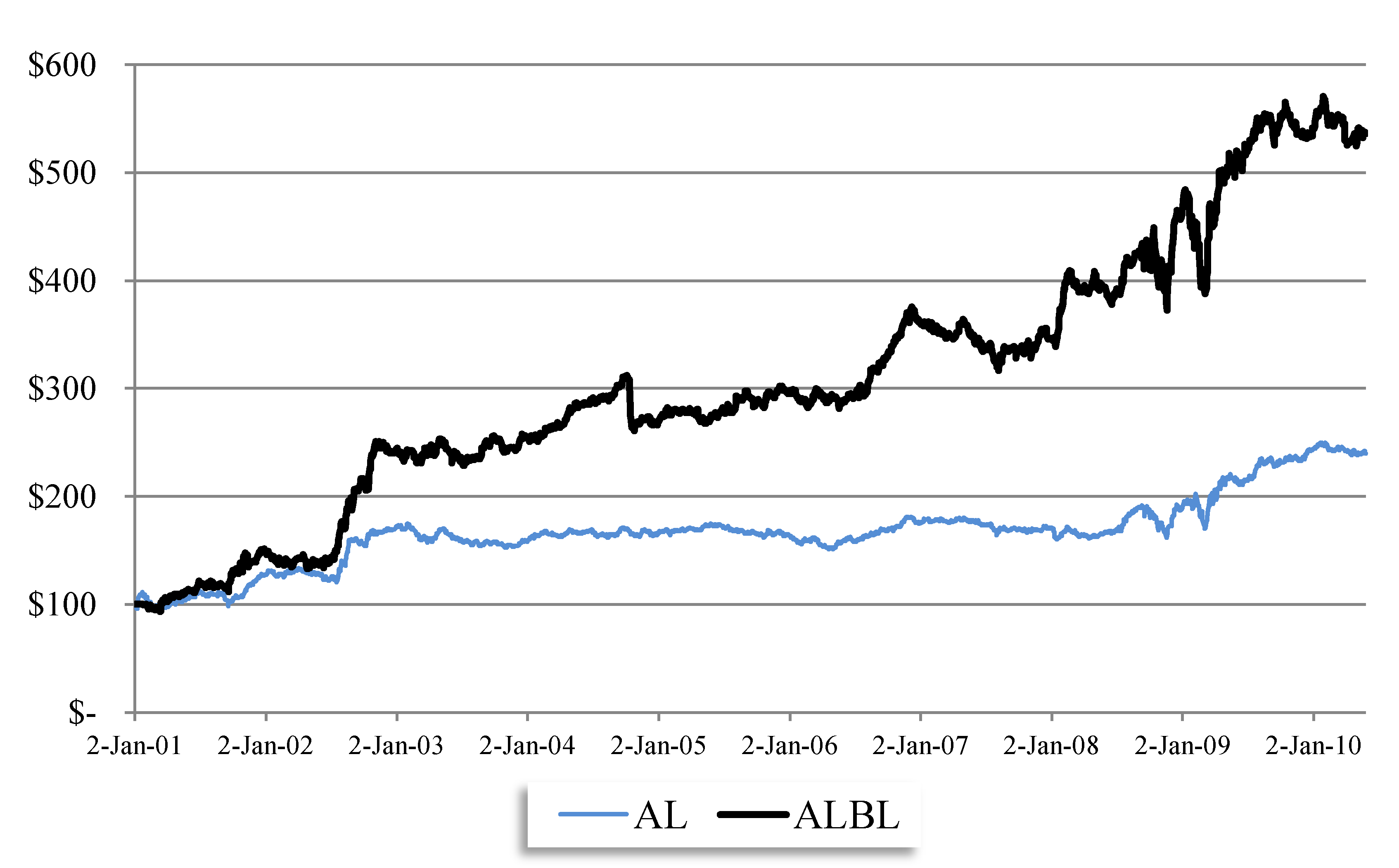
The main results are highlighted in Figure 1 below. We find that the ALBL strategy significantly outperforms the AL investment strategy. Figure 1 displays the performance net of costs for ALBL vs. AL over the period from January 2, 2001 to May 27, 2010. Assuming a zero risk free rate, we compute the Sharpe Ratio of AL to be 0.843, compared to that of ALBL which is 1.225, which is an increase of over 45%. Incidentally, we also find that the daily rolling 3-year Sharpe Ratio of ALBL is consistently above that of the AL strategy (results available upon request).
The remainder of this paper is organized as follows: Section 3 and Section 4, we begin with a short discussion on the ALBL model. Section 5, we discuss issues with proper back-testing procedures as well as describing our data and the many associated biases. Section 7 and Section 8, we discuss our results. Section 9, we conclude with thoughts for the future of the “focused-core” hedge fund strategies.
Figure 1.
Historical Performance Net of Costs: Avellaneda and Lee methodology/Black and Litterman framework (ALBL) vs. Avellaneda and Lee methodology (AL). Time Period: January 2, 2001 to May 27, 2010.
Figure 1.
Historical Performance Net of Costs: Avellaneda and Lee methodology/Black and Litterman framework (ALBL) vs. Avellaneda and Lee methodology (AL). Time Period: January 2, 2001 to May 27, 2010.

3. The Mean-Reversion Model
Mean-reversion or contrarian strategies are based on price movements in which prices stray too far away from some original level and then tend to revert back to normalcy. Some industry experts explain this phenomenon by large institutional buying/selling demands that push the prices away from equilibrium values. The participants that provide liquidity in these periods receive, in an efficiently functioning market, a premium associated with providing liquidity during these times. The opposite of a mean-reversion or contrarian strategy would be a momentum or trending-following strategy, which holds that when, prices move in a particular direction they will continue and not revert. Incidentally, a momentum strategy becomes much more difficult to properly back-test as prices drift higher/lower when a buy/sell order is generated. Chasing the market is much more difficult than providing liquidity against the market direction.
In this section we summarize the AL strategy. AL has an elegant approach by assuming the OU process on the co-integration residuals.
The OU process, Xi(t), being defined as follow:
ki is the speed of reversion to the long-term mean mi, with σi the volatility of the OU process of security i, and we assume we have N securities. W(t) is the standard Brownian motion.
dXi(t) = ki(mi - Xi(t))dt + σidWi(t), with ki > 0
The residuals are obtained from the first step of regressing stock i’s returns on the respective stock i’s sector ETF returns.
![Risks 01 00162 i002]() where α is the estimated intercept of the regression and β is the estimated slope coefficient obtained from the regression. ϵt is the residual at time t obtained from the regression for stock i. AL sets the number of daily observation employed in the regression to be 60 days, additionally they examine when the independent variable is set to certain number of principal components. In this paper we will only examine the case using stock’s sector ETFs.
where α is the estimated intercept of the regression and β is the estimated slope coefficient obtained from the regression. ϵt is the residual at time t obtained from the regression for stock i. AL sets the number of daily observation employed in the regression to be 60 days, additionally they examine when the independent variable is set to certain number of principal components. In this paper we will only examine the case using stock’s sector ETFs.

The second step is to define the sum of residuals process for stock i at time t:
![Risks 01 00162 i003]() OU parameters are obtained from assuming an AR(1) process and estimating the coefficients in a lag 1 regression model employing the prior 59 observations of
OU parameters are obtained from assuming an AR(1) process and estimating the coefficients in a lag 1 regression model employing the prior 59 observations of ![Risks 01 00162 i019]() :
:
![Risks 01 00162 i004]() whereby:
whereby:
![Risks 01 00162 i006]()
![Risks 01 00162 i007]()
![Risks 01 00162 i008]() We arrive with our s-score:
We arrive with our s-score:
![Risks 01 00162 i009]()

 :
:

ki = −log(b)252


Finally, similar to AL we incorporate the “trade” time weighing scheme for returns.
4. Black–Litterman Framework and Active Mean-Reversion Management
In this section, we detail the ALBL model by demonstrating how AL’s OU mean-reversion process maps naturally within BL framework for portfolio allocation.
BL attempts to stabilize the optimal portfolio allocations by blending the equilibrium (excess) expected returns vectors with a view vector. We assume we have N assets. It is well-known that the solution to the unconstrained optimization problem is sensitive to perturbation in.μ
![Risks 01 00162 i010]() with μ the (N × 1) expected return vector, ∑ the (N × N) variance-covariance matrix of returns, and λ the risk aversion coefficient. The unconstrained solution is. ω = (λ∑)−1μ Notice that the optimal weights are linear in μ and inversely related to λ, ceteris paribus. BL invert this optimal solution to derive the equilibrium expected return vector by replacing the ω with the market observed vector of weights, ωmkt BL begins by defining the equilibrium expected returns as follows:
Additionally, ∑ the covariance matrix is typically measured employing historical returns data. In order to stabilize the original μ vector of expected returns, BL blends П with views vector, q , thereby limiting the movement of the expected return vector and thus keeping the optimal solution, ω, relatively well-behaved. It becomes a bit more clear, if we assume we have N absolute views so q is (N × 1), we can write the posterior expected return, E(r), as the weighted sum of equilibrium expected returns, П, and views, q :
with μ the (N × 1) expected return vector, ∑ the (N × N) variance-covariance matrix of returns, and λ the risk aversion coefficient. The unconstrained solution is. ω = (λ∑)−1μ Notice that the optimal weights are linear in μ and inversely related to λ, ceteris paribus. BL invert this optimal solution to derive the equilibrium expected return vector by replacing the ω with the market observed vector of weights, ωmkt BL begins by defining the equilibrium expected returns as follows:
Additionally, ∑ the covariance matrix is typically measured employing historical returns data. In order to stabilize the original μ vector of expected returns, BL blends П with views vector, q , thereby limiting the movement of the expected return vector and thus keeping the optimal solution, ω, relatively well-behaved. It becomes a bit more clear, if we assume we have N absolute views so q is (N × 1), we can write the posterior expected return, E(r), as the weighted sum of equilibrium expected returns, П, and views, q :
![Risks 01 00162 i011]() In general, we define the following as:
In general, we define the following as:

П = λ∑ωmkt

| П | N × 1, vector of equilibrium expected returns, which is assumed to be known; |
| ∑ | N × N, covariance matrix of returns, which, again, is assumed to be known; |
| Ρ | K × N, pick matrix; |
| q | K × 1, vector of views on the returns; |
| Ω | K × K, diagonal covariance matrix that expresses the confidence in the views (the stronger the view, the smaller the corresponding entry); |
| E(r) | N × 1, the resulting expected return vector after incorporating our views; |
| τ | 1 × 1, the measure of the uncertainty of the prior estimate of the mean returns. |
We do not go into all the details of the BL model interested reader should see He and Litterman [1], but only list the model parameters and provide a discussion on how to set these parameters from our mean-reversion model. Throughout, we will assume that the investor seeks to construct a market-neutral active portfolio.
4.1. Equilibrium (or Prior) Expected Returns
Following Herold [8] and Da Silva, Lee, and Pornrojnangkool [9] we set the equilibrium expected returns, П, to zero. This falls out directly from the above OU process. In particular, when holding a market-neutral long-short portfolio (assuming α = 0), any net-returns result from the increments of the auxiliary process, dX(t). The increments of the auxiliary process have an unconditional mean equal to zero. Another way to think about this would be that the market processes information correctly when the market is in equilibrium and prices reflect the underlying values so there are no expected profits available to mean-reversion extraction. In cases where there are deviations from equilibrium this may occur due to temporary liquidity demands or other shocks to prices such as major news events, as such these prices may ebb and flow from equilibrium values.
4.2. Covariance Matrix
Again, given our assumption of a market-neutral long-short portfolio, any net-returns result from the increments of the auxiliary process dX(t). We estimate ∑ by the sample covariance matrix from the previous 252 trading days.
4.3. Pick Matrix
BL considers views on expectations. This corresponds to placing views of the expected excess return vector of the assets. In particular, K views represented by a K-by-N pick matrix, P, whose k-th row determines the relative weight of the expected return in the respective view. It is common practice to set this weight to 1 in the case of an absolute view or a combination of 1 and −1 in the case of a relative view. Within our mean-reversion framework, we place an absolute view on each of the assets that we expect to mean-revert. Hence, our pick matrix is simply the identity matrix.
4.4. Views
Our subjective views on the vector of mean excess returns, q, is simply the one-day expected return for each of the assets in our mean-reversion universe. That is, from the above OU-process and the assumption of a market-neutral long-short portfolio, the expected 1-day return on asset i is given by
αidt + ki(mi − Xi(t))dt
4.5. Certainty in Our Views
The diagonal covariance matrix, Ω , is a means to quantify the uncertainty of our views. Let ωi = Ωii. If this value is small, it indicates that there is a large certainty in our in our view and that μi should closely track. qi On the other hand, if ωi is large, it indicates that there is little certainty in our view and that μi should closely track πi. One common method to estimate Ω is as follows:
![Risks 01 00162 i012]() where c represents the overall level of confidence in the views. In this work, we introduce a slightly different approach. We transform the s-scores into confidence intervals which are a monotonically decreasing function that takes quintile s-score values into distinct break-points. The following break-points were employed: [0.1, 0.01, 0.001, 0.0001, 0.00001], with larger/smaller s-score values having a larger/smaller degree of confidence. The idea is to put more emphasis on those s-scores that are larger thus gaining more exposure to those state-of-natures where mean-reversion should occur.
where c represents the overall level of confidence in the views. In this work, we introduce a slightly different approach. We transform the s-scores into confidence intervals which are a monotonically decreasing function that takes quintile s-score values into distinct break-points. The following break-points were employed: [0.1, 0.01, 0.001, 0.0001, 0.00001], with larger/smaller s-score values having a larger/smaller degree of confidence. The idea is to put more emphasis on those s-scores that are larger thus gaining more exposure to those state-of-natures where mean-reversion should occur.

4.6. Posterior Distribution of Expected Returns
From these parameters, the resulting posterior distribution of expected returns μ is a multivariate normal distribution with mean
that can replace the equilibrium expected returns, π, within any asset allocation setting such as Mean-CVaR portfolio optimization or Mean-Variance Optimization.
E(r) = [(τ∑)−1 + PTΩ−1P]−1[(τ∑)−1П + PTΩ−1q]
Following Da Silva, Lee, and Pornrojnangkool [9], with the equilibrium returns set to 0 we arrive at the following problem formulation:
where all other constraints consist of the following:
maxx μTω − λωT∑ω s.t. all other constraints
- Beta-neutrality within each sector
![Risks 01 00162 i015]()
- The sum of all active positions must sum to 0
![Risks 01 00162 i016]()
- Leverage constraints
![Risks 01 00162 i017]()
![Risks 01 00162 i018]() ui ≥ 0 for all i
ui ≥ 0 for all i - Long-only positions for assets we expect to mean-revert from belowωi ≥ 0 for all i ϵ buy to open signal
- Short-only positions for assets we expect to mean-revert from aboveωi ≤ 0 for all i ϵ sell to open signal


5. Discussion on Proper Back-Testing
On several occasions, researchers will find strong back-tested results only to fail when managing “live” capital. One common mistake made when employing returns based on close-to-close prices is “unintentional-cheating.” Suppose that we define P(t) as the closing price at the end of time period t. If we further define returns from end of period t − 1 to end of period t: r(t) = [P(t) / P(t−1)] − 1, then attempt to use r(t) as an input to a model that attempts to gain r(t+1), we would have made the most common back-testing mistake. Namely, we would have assumed that we could have employed P(t) to create our signal and thus our trade-position and then actually traded on P(t), which is a cheat, as r(t+1) = [P(t+1)/P(t)] – 1. We would need to give time for the model to take in the input P(t), process the results and create our position at thus generate the order to trade at a time epsilon greater than t. Of course, epsilon time depends on your infra-structure and locations constraints, etc. In this work, we compute signals using r(t), and book profits at r(t+2). In addition, we assume one-way transaction costs of $1 per ticket charge and $0.003 per share. All results are presented net of these transaction costs unless otherwise specified.
6. Data and Biases
The main source of our data comes from Yahoo! Finance Website [16], which provides daily open, high, low, volume, and adjusted close prices for exchange traded equity securities. We gather our prices from this source which is readily available to all researchers. Below we list some of the potential biases that will affect our results:
- (1)
- Survivorship Bias—we only examine stocks which comprise the ETFs as of May 2010. Therefore, securities that have become defunct over our time period examined are excluded;
- (2)
- Prior Empirical Study Bias—we build upon findings from an earlier empirical study, namely AL. Therefore, there should be no surprise that mean-reversion as defined in the ALBL has worked historically;
- (3)
- Readily Available Data Bias—we examine only securities to which we have readily available data, namely U.S. exchange trade securities available through Yahoo! Finance Website;
- (4)
- Time Period Specific Bias—we focus our study by examining a very limited time period of history: from roughly 2000 to 2010. This period may be very unique and characterized by specific financial events, such as financial market crisis and consequent government intervention, the real estate boom and bust, the quant blow-up, large bankruptcies, etc. Moreover, we only examine daily data so it is unlikely that our results will extend to tick, intraday bars, weekly, monthly, and yearly time-periods;
- (5)
- Unidentified Biases—these include biases that we have not yet identified but which are present in our empirical analysis.
Please note that to the extent that our universe is limited to the larger securities which may be less affected by defunct securities, the survivorship bias may be mitigated. However, to the extent that corporate actions such as merger and acquisitions have consolidated sectors/industries, this bias may be more acute within these sectors. We hope that the above biases will only mitigate and not reverse any of our main results. We are aware and acknowledge that data biases have and continue to refocus our current understanding of empirical research.
7. Discussion of Results I
Our data consists of daily observations from December 31, 1999 to May 27, 2010 or 2,610 possible days. In Table 1, we follow the AL approach by obtaining the respective ETF, employing sector ETFs as our independent variable in our regressions and describing our mean-reversion strategy employed across nine sectors with a 60 day window.
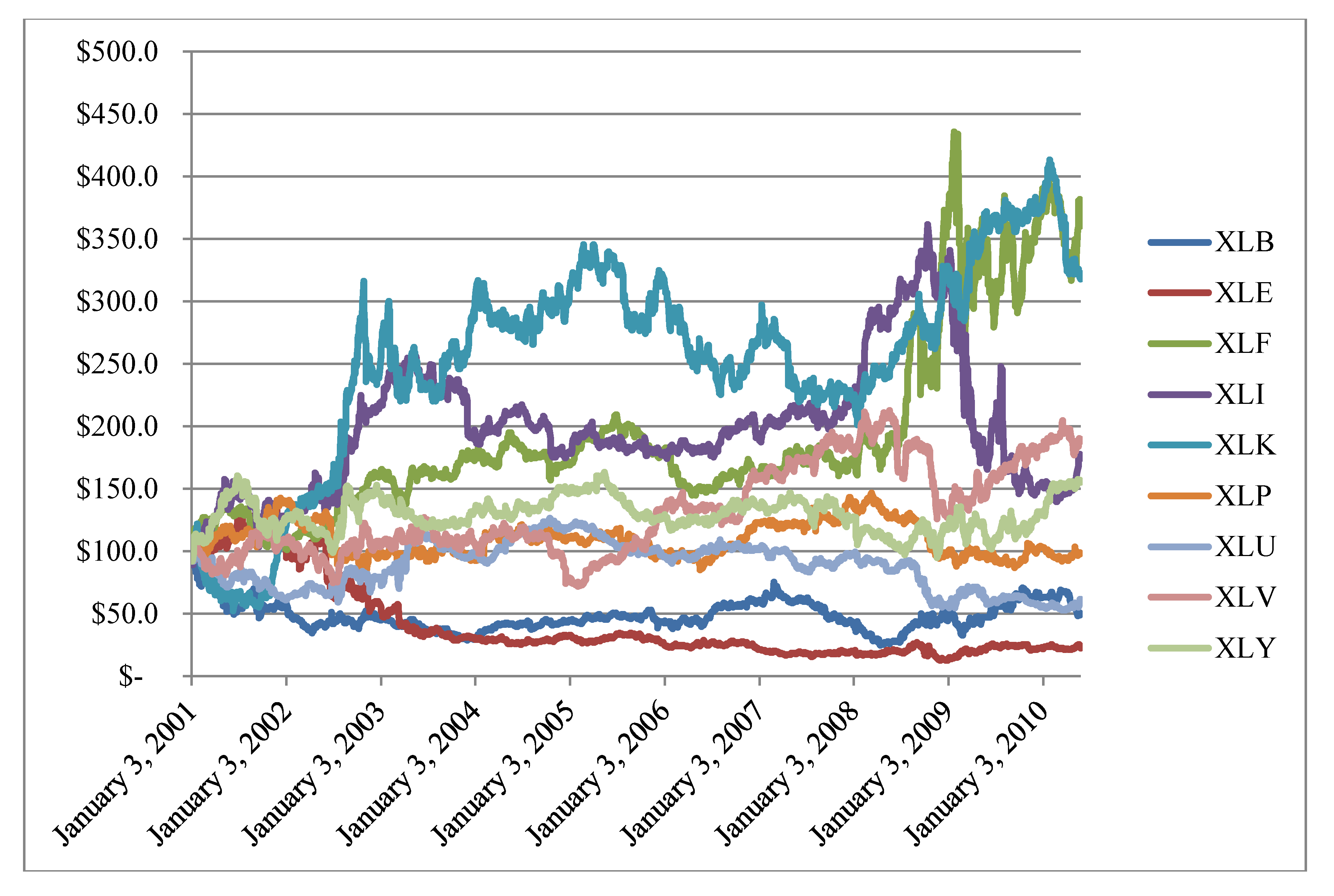
Additionally, we plot the cumulative returns to our sectors in Figure 2. We can see that XLF and XLK are the most profitable sector for mean-reversion extraction with XLB and XLE are the least profitable sectors. Interestingly enough, our strategies are not highly correlated as our cumulative returns appear to have distinct behaviors. Sectors which display mean-reversion with positive drift may have interesting stand-alone investment implications. Additionally, given their low correlations, portfolio of these strategies will benefit from diversification.

Table 1.
Summary statistics of mean-reversion strategy by sector. Ann. Ret.: Annualized Return; Ann. Std.: Annualized Standard Deviation. Sector abbreviations are given in the main text.
| XLB | XLE | XLF | XLI | XLK | XLP | XLU | XLV | XLY | |
| Names | Materials | Energy | Financial | Industrial | Technology | Consumer Staples | Utilities | Health Care | Consumer Discretionary |
| # of Stocks | 31 | 39 | 79 | 57 | 84 | 41 | 36 | 52 | 81 |
| Ann. Ret. | −0.76% | −8.81% | 17.67% | 9.91% | 17.25% | 2.49% | −1.82% | 10.16% | 7.38% |
| Ann. Std. | 36.7% | 37.4% | 27.2% | 28.2% | 31.2% | 22.8% | 25.7% | 25.6% | 23.1% |
| Sharpe (Rf=0) | −0.02 | −0.24 | 0.65 | 0.35 | 0.55 | 0.11 | −0.07 | 0.04 | 0.32 |
| Correlation | XLB | XLE | XLF | XLI | XLK | XLP | XLU | XLV | XLY |
| XLB | 1.00 | 0.03 | 0.06 | 0.05 | 0.03 | 0.03 | 0.03 | 0.03 | 0.07 |
| XLE | 1.00 | 0.04 | 0.04 | −0.02 | −0.01 | 0.05 | 0.00 | 0.03 | |
| XLF | 1.00 | 0.08 | 0.05 | 0.07 | −0.01 | 0.07 | 0.12 | ||
| XLI | 1.00 | 0.04 | 0.05 | 0.06 | 0.06 | −0.01 | |||
| XLK | 1.00 | 0.01 | 0.05 | 0.01 | 0.07 | ||||
| XLP | 1.00 | 0.03 | 0.04 | 0.02 | |||||
| XLU | 1.00 | 0.04 | 0.04 | ||||||
| XLV | 1.00 | 0.05 | |||||||
| XLY | 1.00 |
Figure 2.
Cumulative returns to mean-reversion strategy across nine sectors.

8. Discussion of Results II
Why does mean-reversion work in some sectors and does not work on others?
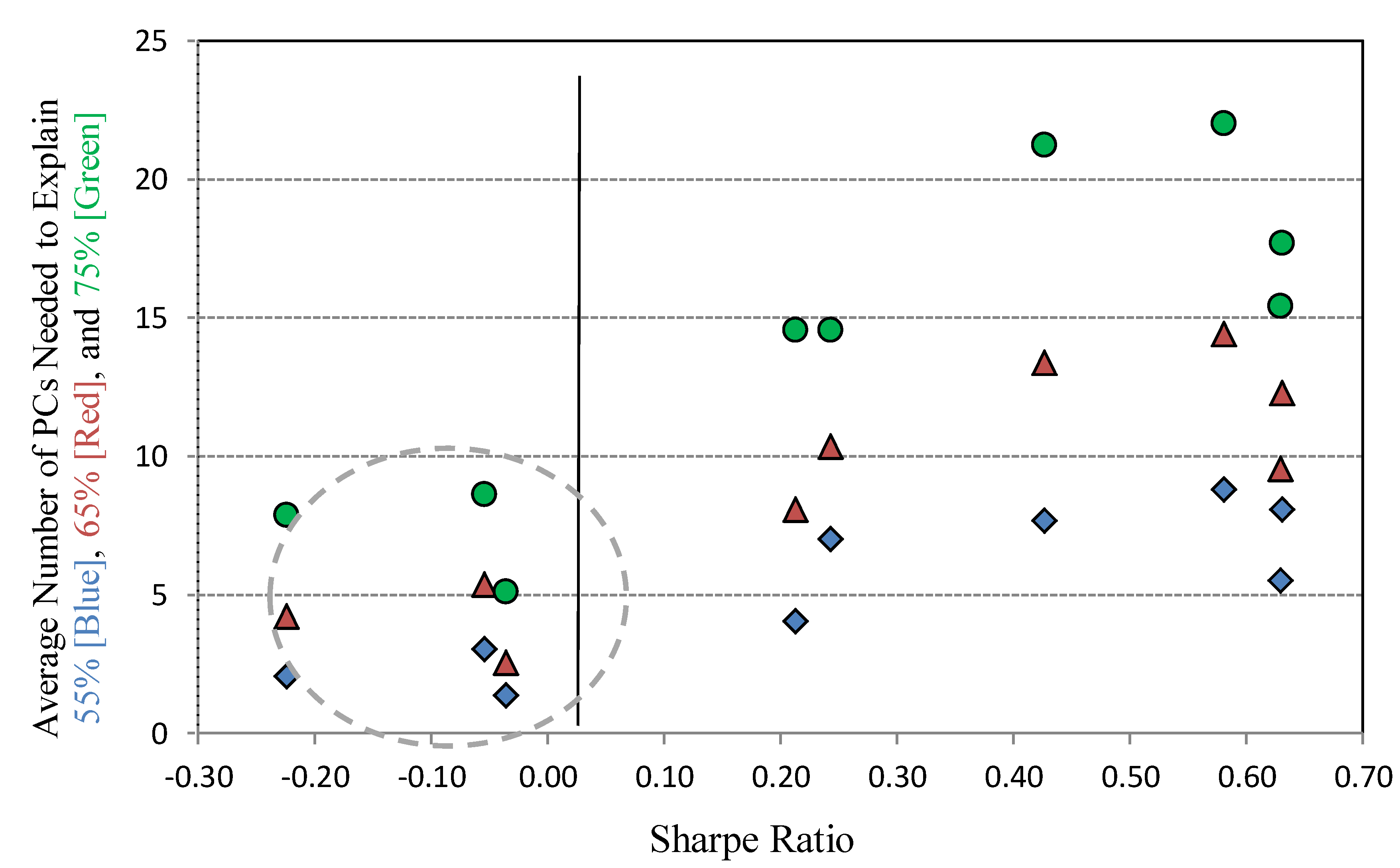
Figure 3 supports the contention that the more PCs (principal components) that are needed to explain the variation of stock returns within a given sector, the more attractive that sector is for mean-reversion extraction. The economic story appears to be that when a sector’s stocks’ risk premium is complicated (i.e., to explain a given level of variation takes relatively more factors), then mean-reversion tends to work better in such sectors. On the contrary, when a sector’s stocks’ risk premium is simple (i.e., to explain a given level of variation takes few factors), then mean-reversion extraction is more difficult. Such observations are important to consider when evaluating if a certain market place is ripe for a mean-reversion strategy. We examined the number of PCs that are required to explain a given level of variations: 55%, 65%, and 75%. We find that sectors that had poor mean-reversion performance also had a very low number of PCs explaining return variation. In particular, the gray circled sectors are Materials, Energy, and Utilities, which all had negative Sharpe Ratios over our sample period.
Figure 3.
Average number of principal components (PCs) needed to explain variation vs. Sharpe ratio.
Figure 3.
Average number of principal components (PCs) needed to explain variation vs. Sharpe ratio.

We began by examining information variables that would help us predict the cross-section of expected mean-reversion returns. We examined many different parameters such as beta, kappa, etc. We found that the absolute value of s-scores helps differentiate the cross-section of returns. Namely, when we sort by absolute value of s-scores, we find that high scores are associated to higher levels of cumulative returns, and lower s-scores with lower cumulative returns. This result led us to incorporate the magnitude of s-score into our confidence parameter—matrix Ω.
We settled on at least one possible explanation, that is, using the absolute value of s-scores will give us more confidence with our views under an OU process framework. That is, we bet more heavily the larger (in absolute sense) the s-score. We examined other functional forms but shall leave this to future research to fine-tune or to optimize our results.
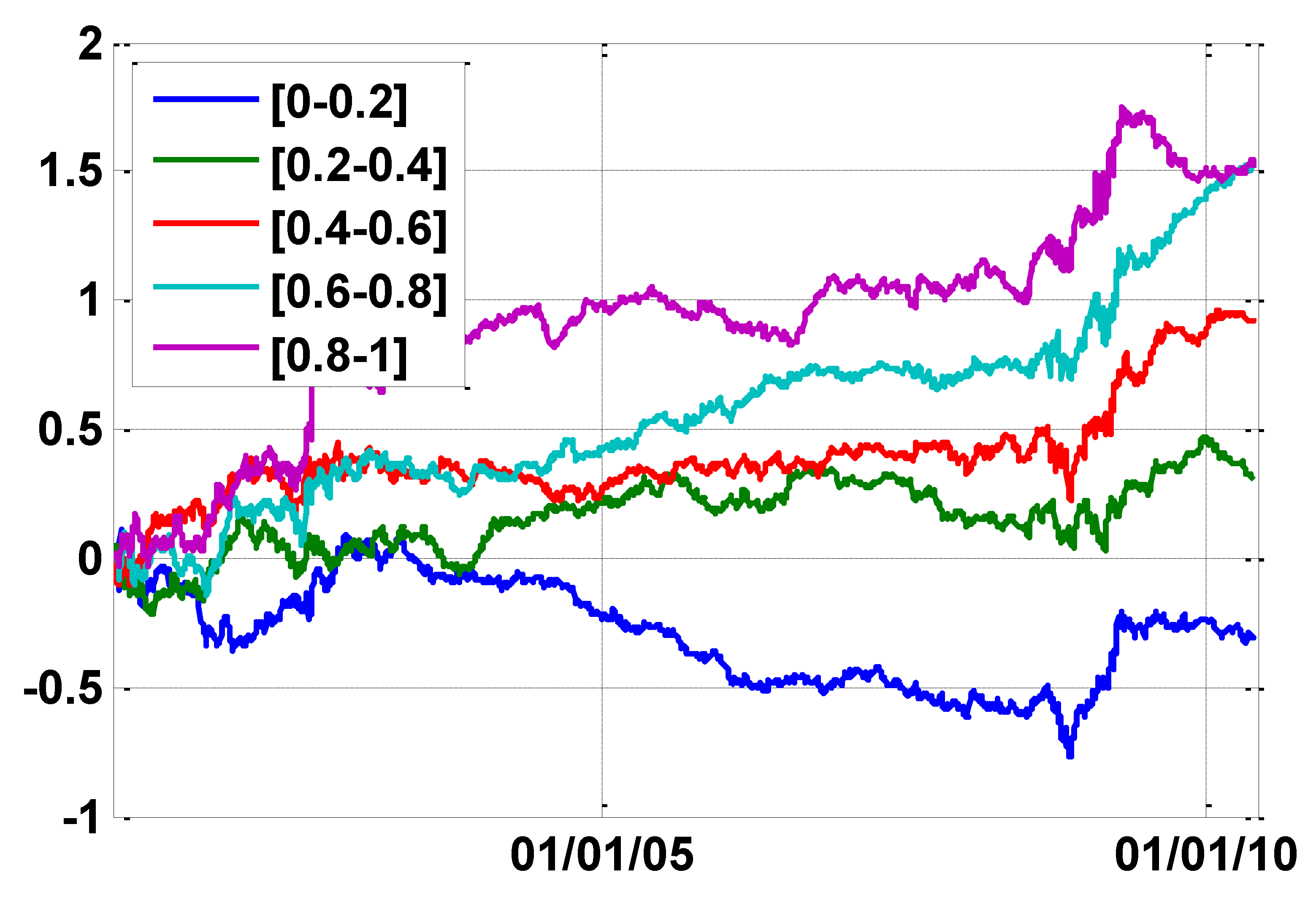
Figure 4 displays quintile portfolio returns sorted by absolute s-score each day. It is apparent that s-scores help to differentiate the cross-section of realized returns, thereby leading us to incorporating this information variable into BL procedure. We sorted our absolute s-scores each day and put them into relative buckets with Blue bucket containing s-scores in the 0%–20% range, Green bucket containing s-score in the 20%–40% range, etc. Next, performance was monitored over time. The purple and light blue lines are associated with the larger absolute s-scores, and blue and green lines are associated with the smaller absolute s-scores.
Figure 4.
S-score quintile performance over time.

9. Conclusion
In this paper, we have introduced a new “focused-core” strategy that attempts to capture the opportunities available employing a fully disclosed transparent mean-reversion strategy trading U.S. equities. In particular, we examine the co-integration residuals under the assumed OU process. Similarly to AL, we employ ETFs as our benchmarks associated with each stock in our universe. We examine a total of 500 stocks. Our model built upon daily data, with all the disclosed biases, but could be easily extended to unbiased data as well as to intra-day data. To the best of our knowledge, we are the first to bridge the gap between transparent statistical arbitrage methodology of AL and institutional-grade asset optimization procedure introduced by BL, thus we formally name this combination as ALBL. The primary endeavor of ALBL is to set the tone for future “focused-core” strategies that are thoughtful in construction and fully disclosed. No doubt many other replicators will emerge, but we feel strongly that such competition within the “focused-core” strategies will be beneficial to our industry, as well as to institutional investors. If in fact such “focused-core” strategies capture a significant portion of the return generating process of statistical arbitrage hedge funds, then institutional investors should expect lower fees and more transparency in the near future.
Acknowledgments
We would like to thank Brian Hayes, Sumit Kumar Jha, Joy Pathak, Min Shin, and Achilles Venetoulias for helpful comments and suggestions. All remaining errors are our own.
References
- G. He, and R. Litterman. “The Intuition Behind Black–Litterman Model Portfolio.” San Fransisco, CA, USA: Goldman Sachs, Investment Management Division, 1999. [Google Scholar]
- M.J. Poterba, and L.H. Summers. “Mean reversion in stock prices: Evidence and implications.” J. Financ. Econ. 22 (1988): 27–59. [Google Scholar] [CrossRef]
- E.F. Fama, and K.R. French. “Common risk factors in the returns on stocks and bonds.” J. Financ. Econ. 33 (1993): 3–56. [Google Scholar] [CrossRef]
- E.F. Fama, and K.R. French. “Luck vs. skill in the cross section of mutual fund returns.” J. Financ. 65 (2010): 1915–1947. [Google Scholar] [CrossRef]
- M. Carhart. “On persistence in mutual fund performance.” J. Financ. 52 (1997): 57–82. [Google Scholar] [CrossRef]
- M. Avellaneda, and J.H. Lee. “Statistical arbitrage in the U.S. equity market.” Quant. Financ. 10 (2010): 761–782. [Google Scholar] [CrossRef]
- F. Black, and R. Litterman. “Asset allocation: Combining investors’ views with market equilibrium.” J. Fixed Income 1 (1991): 7–18. [Google Scholar] [CrossRef]
- F. Black, and R. Litterman. “Global portfolio optimization.” Financ. Anal. J. 48 (1992): 28–43. [Google Scholar] [CrossRef]
- U. Herold. “Portfolio construction with qualitative forecasts.” J. Portfolio Manag. 30 (2003): 61–72. [Google Scholar] [CrossRef]
- A.S. Da Silva, W. Lee, and B. Pornrojnangkool. “The Black–Litterman model for active portfolio management.” J. Portfolio Manag. 35 (2009): 61–70. [Google Scholar]
- E.G. Uhlenbeck, and L.S. Ornstein. “On the theory of the Brownian motion.” Phys. Rev. 36 (1930): 823–841. [Google Scholar] [CrossRef]
- W.A. Lo, and A.C. MacKinlay. “When are contrarian profits due to stock market overreaction? ” Rev. Financ. Stud. 3 (1990): 175–205. [Google Scholar] [CrossRef]
- N. Jegadeesh, and S. Titman. “Returns to buying winners and selling losers: Implications for stock market efficiency.” J. Financ. 48 (1993): 65–91. [Google Scholar] [CrossRef]
- N. Jegadeesh, and S. Titman. “Overreaction, delayed reaction, and contrarian profits.” Rev. Financ. Stud. 8 (1995): 973–993. [Google Scholar] [CrossRef]
- S. Satchell, and A. Scowcroft. “A demystification of the Black–Litterman model: Managing quantitative and traditional portfolio construction.” J. Asset Manag. 1 (2000): 138–150. [Google Scholar] [CrossRef]
- T. Idzorek. “A Step-by-Step Guide to the Black–Litterman Model.” In Forecasting Expected Returns in the Financial Markets. Edited by S. Satchell. Waltham, MA, USA: Academic Press, 2007. [Google Scholar]
- “Yahoo! Finance Website.” Available online: http://finance.yahoo.com (accessed on 1 October 2013).
© 2013 by the authors; licensee MDPI, Basel, Switzerland. This article is an open access article distributed under the terms and conditions of the Creative Commons Attribution license (http://creativecommons.org/licenses/by/3.0/).
Share and Cite
MDPI and ACS Style
Liew, J.; Roberts, R. U.S. Equity Mean-Reversion Examined. Risks 2013, 1, 162-175. https://doi.org/10.3390/risks1030162
AMA Style
Liew J, Roberts R. U.S. Equity Mean-Reversion Examined. Risks. 2013; 1(3):162-175. https://doi.org/10.3390/risks1030162
Chicago/Turabian StyleLiew, Jim, and Ryan Roberts. 2013. "U.S. Equity Mean-Reversion Examined" Risks 1, no. 3: 162-175. https://doi.org/10.3390/risks1030162