Gaussian and Affine Approximation of Stochastic Diffusion Models for Interest and Mortality Rates

Abstract

In the actuarial literature, it has become common practice to model future capital returns and mortality rates stochastically in order to capture market risk and forecasting risk. Although interest rates often should and mortality rates always have to be non-negative, many authors use stochastic diffusion models with an affine drift term and additive noise. As a result, the diffusion process is Gaussian and, thus, analytically tractable, but negative values occur with positive probability. The argument is that the class of Gaussian diffusions would be a good approximation of the real future development. We challenge that reasoning and study the asymptotics of diffusion processes with affine drift and a general noise term with corresponding diffusion processes with an affine drift term and an affine noise term or additive noise. Our study helps to quantify the error that is made by approximating diffusive interest and mortality rate models with Gaussian diffusions and affine diffusions. In particular, we discuss forward interest and forward mortality rates and the error that approximations cause on the valuation of life insurance claims.

1. Introduction

For the most part of the 20th century, actuaries used to model the lifespan of an insured stochastically, but relied on a mere deterministic prognosis of capital returns and mortality rates. The past has shown that these assumptions can vary significantly within one contract period. Especially in recent years, financial markets have experienced increased volatility, and life expectancies have risen in many developed countries at an unforeseen rate. For two decades, actuaries have been increasingly using stochastic interest rate models, and since the last decade, stochastic mortality rate models have become more and more popular. On the one hand, the stochastic approach helps to better capture systematic risk by offering the possibility to calculate confidence intervals. On the other hand, investors and insurance regulators nowadays call for a market-consistent valuation of the insurers assets and liabilities, so that concepts from financial mathematics have entered actuarial science, where the market value of a claim is calculated as a risk-neutral expectation in a specific stochastic model.

In financial mathematics, stochastic modeling of interest rates is a common approach, and a great variety of different interest rate models can be found in the literature. The majority of authors models the interest rate with the help of diffusion processes. Typical short rate models are, for example, the Vasicek model and the Cox–Ingersoll–Ross model. The evolution of forward rates is often modeled within the Heath–Jarrow–Morton framework. Readers may refer to [1] for a comprehensive overview or to the original works, such as [2,3,4]. In the nineteen nineties, these models also found their way into the actuarial literature; see e.g., [5,6,7,8,9,10,11].

The uncertainty about future mortality probabilities always drew the attention of life insurance actuaries. However, since recently, actuaries have been increasingly using stochastic models for the mortality rate. A very popular approach is to adopt the well-known models from interest rate theory, such as the Vasicek or the Cox–Ingersoll–Ross model. A more recent development is the concept of forward mortality rates, which are frequently modeled by a Heath–Jarrow–Morton framework similarly to forward interest rates. References that use diffusion process are, e.g., [12,13,14,15,16,17,18,19,20,21,22,23,24], just to mention a few. Although negative mortality rates do not have a meaningful interpretation, many of those references use diffusion models, where negative values occur with a positive probability. In particular, Gaussian diffusion processes are frequently used. This is justified with the argument that Gaussian models would offer a good approximation of more appropriate models.

In the present paper, we study the asymptotics of diffusions with affine drift and a general noise term to corresponding diffusions with an affine drift term, but an affine noise term or additive noise. In the additive case, we end up with Gaussian processes, that is, the finite-dimensional projections are multivariate, normally distributed. The affine case is a generalization of the additive case and allows for better approximations, but the corresponding distributions are not always analytically tractable. We introduce a reasonable approximation concept and calculate bounds for the absolute moments of the approximation errors. Furthermore, we calculate the error that the approximating processes imply when valuating insurance claims. Our basic notion is to study asymptotics relative to the size of the noise term; the smaller the noise term, the better the approximation. Our results help to better assess the quality of Gaussian and affine approximations for interest and mortality rate models.

After introducing a basic life insurance model in Section 2, we study Gaussian approximations in Section 3 and affine approximations in Section 4 and present theoretical results for the asymptotic behavior. The proofs are put into their own section at the end; see Section 7. In Section 5, we discuss the effect of the Gaussian and affine approximations on the valuation of insurance claims. A numerical illustration is given in Section 6. In Section 8, we summarize our findings.

2. Basic Life Insurance Framework

Assume that the lifetime of a policyholder is described by a nonnegative random variable T. Time t measures the seniority of the policy (i.e., the time elapsed since policy issue). Policyholder’s age at policy issue is denoted as x, so that the age at time t is $x+t$. Suppose that the distribution function $P[T\le x+t]$ of the lifetime T has a representation of the form:

$$\begin{array}{c}\hfill 1-e^{-{\int }_0^{x+t}m\left(s\right)\text{d}s}\end{array}$$

(1)

where m is the so-called mortality rate (or force of mortality). We consider a general life insurance contract with both survival and death benefits. We write $B\left(t\right)$ for the aggregated survival benefits minus premiums on $[0,t]$ and $c\left(t\right)$ for the benefit payments that are due in the case of a death at time t. The contract terminates at time ${\omega }_x=\omega -x<\infty$, at the latest, where ω is the maximal value that T can take, possibly infinite.

Let $r\left(t\right)$ be the short rate. Then, the discounted sum of future benefits minus premiums for a policyholder alive at time t is given by:

$$\begin{array}{c}\hfill A\left(t\right)={\int }_{(t,T)}{e}^{-{\int }_t^{s}r\left(u\right)\text{d}u}\text{d}B\left(s\right)+e^{-{\int }_t^{T}r\left(u\right)\text{d}u}c\left(T\right).\end{array}$$

(2)

In classical life insurance modeling, r and m are integrable functions, B is a right-continuous function with finite variation and c is a bounded function. Therefore, in the classical perspective, r, m, B and c are deterministic, and the prospective reserve at time t in the active state is defined as:

$$\begin{array}{cc}\hfill V(t;r,m)& =E\left[A\right(t)|T>t]\hfill \end{array}$$

(3)

and has the representation:

$$\begin{array}{cc}\hfill V(t;r,m)& ={\int }_{(t,{\omega }_x]}{e}^{-{\int }_t^{s}r\left(u\right)+m(x+u)\text{d}u}\text{d}B\left(s\right)+{\int }_t^{{\omega }_x}{e}^{-{\int }_t^{s}r\left(u\right)+m(x+u)\text{d}u}m(x+s)c\left(s\right)\text{d}s.\hfill \end{array}$$

(4)

In insurance practice, the functions r and m are not perfectly known for the future, but have to be forecasted. In order to capture the corresponding uncertainty, we construct a doubly-stochastic model by assuming that:

• ${\left(r\left(t\right)\right)}_{t\ge 0}$ is a stochastic process with continuous paths,
• ${\left(m\left(t\right)\right)}_{t\ge 0}$ is a stochastic process with continuous paths,
• ${\left({\mathcal{F}}_t\right)}_{t\ge 0}$ is the natural filtration generated by the joint process, $(r,m)$.

Let ${\mathcal{F}}_{\infty }:=\sigma \left({\bigcup }_{t\ge 0}{\mathcal{F}}_t\right)=\sigma (r\left(t\right),m\left(t\right),t\ge 0)$. We can embed the classical model, where r and m are deterministic, into the doubly-stochastic model by interpreting Formula (1) as the conditional distribution function $P[T\le x+t|{(r\left(t\right),m\left(t\right))}_{t\ge 0}]:=P[T\le x+t|{\mathcal{F}}_{\infty }]$. Doing that for all $x+t$, Formula (1) uniquely defines a stochastic kernel $(A,(r,m))\mapsto P[T\in A|{(r\left(t\right),m\left(t\right))}_{t\ge 0}=(r,m)]$. The prospective reserve according to Equation (4) is now interpreted as the conditional expectation:

$$\begin{array}{cc}\hfill V(t;r,m)& =E[A\left(t\right)|T>t,{(r\left(t\right),m\left(t\right))}_{t\ge 0}=(r,m)].\hfill \end{array}$$

(5)

Moreover, B and c may here be ${\left({\mathcal{F}}_t\right)}_{t\ge 0}$-adapted stochastic processes, as well. For a rigorous definition of the integrals in Equation (4), we assume that B is a semimartingale and c, a bounded process. In the following, we work throughout in the doubly-stochastic framework.

Suppose that we are at time s, where the information ${\mathcal{F}}_s$ is available. The forward interest rate, ${\left({\rho }_s\left(t\right)\right)}_{t\ge s}$, is defined via a zero-coupon bond, i.e., as the ${\mathcal{F}}_s$-measurable solution of:

$$\begin{array}{c}\hfill E\left[e^{-{\int }_s^{t}r\left(u\right)\text{d}u}|{\mathcal{F}}_s\right]=e^{-{\int }_s^t{\rho }_s\left(u\right)\text{d}u},t\ge s\end{array}$$

(6)

where the underlying probability measure represents here some market measure. In the present paper, we suppose throughout that the underlying probability measure is given by the context of the application and that in the following all expectations are calculated on the basis of that probability measure. For our asymptotic approximation results, the origin of the underlying probability measure will not be relevant. In [12,13,16,19], a forward mortality rate ${\left({\mu }_s\left(t\right)\right)}_{t\ge s}$ is defined as the ${\mathcal{F}}_s$-measurable solution of:

$$\begin{array}{c}\hfill E\left[e^{-{\int }_s^{t}m\left(u\right)\text{d}u}|{\mathcal{F}}_s\right]=e^{-{\int }_s^t{\mu }_s\left(u\right)\text{d}u},t\ge s.\end{array}$$

(7)

In [25], we find a spread rate concept where the forward mortality rate is either defined as the solution of:

$$\begin{array}{c}\hfill E\left[e^{-{\int }_s^{t}r\left(u\right)+m\left(u\right)\text{d}u}|{\mathcal{F}}_s\right]=e^{-{\int }_s^t{\rho }_s\left(u\right)+{\mu }_s\left(u\right)\text{d}u},t\ge s\end{array}$$

(8)

or as the solution of:

$$\begin{array}{c}\hfill E\left[{\int }_s^t{e}^{-{\int }_s^{\tau }r\left(u\right)+m\left(u\right)\text{d}u}m\left(\tau \right)\text{d}\tau |{\mathcal{F}}_s\right]={\int }_s^t{e}^{-{\int }_s^{\tau }{\rho }_s\left(u\right)+{\mu }_s\left(u\right)\text{d}u}{\mu }_s\left(\tau \right)\text{d}\tau ,t\ge s.\end{array}$$

(9)

3. Gaussian Diffusion Approximation

In this section, we discuss in some generality the approximation of diffusions with affine drift and a general noise term by corresponding Gaussian diffusions with an affine drift term and additive noise.

Let X be a diffusion process that satisfies the stochastic differential equation

$$\begin{array}{c}\hfill \text{d}X\left(t\right)=\left(\alpha \left(t\right)X\left(t\right)+\beta \left(t\right)\right)\text{d}t+\varsigma \sigma (X\left(t\right),t)\text{d}W\left(t\right),t\ge 0,X\left(0\right)=x_0\in \mathbb{\text{R}}\end{array}$$

(10)

where $\varsigma \in [0,1]$ is a scaling parameter and:

(a)

the column vector $W\left(t\right)$ is a d-dimensional standard Wiener process, $d\in \mathbb{\text{N}}$,

(b)

the mapping, $(x,t)\mapsto \alpha (x,t)x+\beta \left(t\right)$, which is composed of the bounded and measurable mappings $\alpha :[0,\omega ]\to \mathbb{\text{R}}$ and $\beta :[0,\omega ]\to \mathbb{\text{R}}$, is jointly measurable on $\mathbb{\text{R}}\times [0,\omega ]$,

(c)

the mapping $\sigma :\mathbb{\text{R}}\times [0,\omega ]\to {\mathbb{\text{R}}}^{1\times d}$ is jointly measurable on $\mathbb{\text{R}}\times [0,\omega ]$,

(d)

there exists a constant $K>0$, such that

$$\parallel \sigma (x,t)-\sigma (y,t)\parallel \le {K|x-y|,\parallel \sigma (x,t)\parallel }^2\le K^2{(1+|x|}^2)$$

for all $x,y\in \mathbb{\text{R}}$, $t\in [0,\omega ]$, where $\parallel ·\parallel$ is the Euclidean norm.

These assumptions are sufficient to ensure that the stochastic differential equation according to (10) has a unique solution with finite moment functions of any order; see Section 4.5 in [26]. As the $dt$ term in Equation (10) can be seen as an affine mapping of $X\left(t\right)$, we say that X has an affine drift term. The scaling parameter, ς, will be the reference parameter for studying asymptotic properties of X. For $\varsigma =0$, we obtain the differential equation of the expectation function, $E\left[X\right(t\left)\right]$, of $X\left(t\right)$:

$$\begin{array}{c}\hfill \text{d}E\left[X\left(t\right)\right]=\left(\alpha \left(t\right)E\left[X\right(t\left)\right]+\beta \left(t\right)\right)\text{d}t,t\ge 0,E\left[X\left(0\right)\right]=x_0.\end{array}$$

(11)

To see that this is indeed the differential equation of the expectation function, integrate Equation (10) from zero to t; take expectation, and then, differentiate again. Apart from a few specific choices of σ, the distribution of X is not analytically tractable. Calculations are much easier if $\sigma \left(X\right(t),t)$ is deterministic, since then, X satisfies a stochastic differential equation with so-called additive noise, and X is a Gaussian process, i.e., its finite dimensional projections are multivariate, normally distributed. With respect to the mean squared error, the best deterministic substitute for $\sigma \left(X\right(t),t)$ is $E\left[\sigma \right(X\left(t\right),t\left)\right]$, as the following proposition shows.

Proposition 3.1. Let the process $X^{*}$ be defined by:

$$\begin{array}{c}\hfill \text{d}{X}^{*}\left(t\right)=\left(\alpha \left(t\right)X^{*}\left(t\right)+\beta \left(t\right)\right)\text{d}t+\varsigma E\left[\sigma (X\left(t\right),t)\right]\text{d}W\left(t\right),t\ge 0,X^{*}\left(0\right)=x_0\in \mathbb{\text{R}}\end{array}$$

(12)

and for a bounded and measurable function $S:[0,\omega ]\to {\mathbb{\text{R}}}^{1\times d}$, let Y be a process defined by:

$$\begin{array}{c}\hfill \text{d}Y\left(t\right)=\left(\alpha \left(t\right)Y\left(t\right)+\beta \left(t\right)\right)\text{d}t+\varsigma S\left(t\right)\text{d}W\left(t\right),t\ge 0,Y\left(0\right)=y_0.\end{array}$$

(13)

Then, for all choices of $y_0$ and S, we have:

$$\begin{array}{c}\hfill E\left[{(X\left(t\right)-X^{*}\left(t\right))}^2\right]\le E\left[{(X\left(t\right)-Y\left(t\right))}^2\right].\end{array}$$

(14)

Proof. By applying Ito’s formula:

$$\begin{array}{cc}\hfill {(X\left(t\right)-Y\left(t\right))}^2=& {(x_0-y_0)}^2+{\int }_0^{t}2(X\left(s\right)-Y\left(s\right))\alpha \left(s\right)\text{d}s\hfill \\ & +\frac{1}{2}{\int }_0^{t}2{\varsigma }^2{\parallel \sigma (X\left(s\right),s)-S\left(s\right)\parallel }^2\text{d}s+{\int }_0^t...\text{d}W\left(s\right)\hfill \end{array}$$

(15)

and taking expectations on both sides, we obtain:

$$\begin{array}{cc}\hfill E\left[{(X\left(t\right)-Y\left(t\right))}^2\right]=& {(x_0-y_0)}^2+{\int }_0^{t}2E\left[{(X\left(s\right)-Y\left(s\right))}^2\right]\alpha \left(s\right)\text{d}s\hfill \\ & +{\int }_0^t{\varsigma }^{2}E[\parallel \sigma (X\left(s\right),s)-S\left(s\right)]{\parallel }^2]\text{d}s.\hfill \end{array}$$

(16)

The latter integral equation has the unique solution:

$$\begin{array}{c}\hfill E\left[{(X\left(t\right)-Y\left(t\right))}^2\right]=e^{{\int }_0^{t}2\alpha \left(s\right)\text{d}s}\left({(x_0-y_0)}^2+{\int }_0^t{e}^{-{\int }_0^{s}2\alpha \left(u\right)\text{d}u}{\varsigma }^{2}E[\parallel \sigma (X\left(s\right),s)-S\left(s\right)]{\parallel }^2]\text{d}s\right).\end{array}$$

(17)

The right-hand side is minimal if $x_0$ equals $y_0$ and $S\left(s\right)$ equals $E\left[\sigma \right(X\left(s\right),s\left)\right]$, since:

$$\begin{array}{c}\hfill {E[\parallel \sigma (X\left(s\right),s)-S\left(s\right)]\parallel }^2{]=E[\parallel \sigma (X\left(s\right),s)-E\left[\sigma (X\left(s\right),s)\right]\parallel }^2{]+\parallel E\left[\sigma (X\left(s\right),s)\right]-S\left(s\right)\parallel }^2.\end{array}$$

(18)

☐

In the insurance applications that we have in mind, the distribution of X is difficult to get, and so, we also have difficulties in calculating $E\left[\sigma \right(X\left(t\right),t\left)\right]$. Therefore, we suggest approximating X by substituting $\sigma \left(X\right(t),t)$ with $\sigma \left(E\right[X\left(t\right)],t)$ instead of $E\left[\sigma \right(X\left(t\right),t\left)\right]$, which leads to a Gaussian diffusion $\tilde{X}$, defined by:

$$\begin{array}{c}\hfill \text{d}\tilde{X}\left(t\right)=\left(\alpha \left(t\right)\tilde{X}\left(t\right)+\beta \left(t\right)\right)\text{d}t+\varsigma \sigma (E\left[X\left(t\right)\right],t)\text{d}W\left(t\right),t\ge 0,\tilde{X}\left(0\right)=x_0.\end{array}$$

(19)

Note that the expectation functions of $\tilde{X}$ and X are equal and that they can be easily obtained from Equation (11). If the difference between $X\left(t\right)$ and $E\left[X\right(t\left)\right]$ is small, then $\tilde{X}$ should be a good approximation for X. The fluctuation of $X\left(t\right)-E\left[X\right(t\left)\right]$ is small whenever ς is small, because a small ς means that we have only little noise. The following theorem gives an asymptotic result on the absolute moments of the approximation error $X\left(t\right)-\tilde{X}\left(t\right)$.

Theorem 3.2. Assume that the properties (a) to (d) hold. Then, for each $(k,l)\in {\mathbb{\text{N}}}_0^2$, there exists a constant $C_{kl}<\infty$ in such a way that:

$$\begin{array}{c}\hfill \mathbb{\text{E}}\left[|X\left(t\right)-\tilde{X}{\left(t\right)|}^k{|X\left(t\right)-E\left[X\left(t\right)\right]|}^l\right]\le C_{k,l}{\varsigma }^{2k+l},\mathrm{for}\mathrm{all}t\in [0,\omega ],0\le \varsigma \le 1.\end{array}$$

(20)

For the proof, see Section 7. From this theorem, we learn that approximating $X\left(t\right)$ by its expectation function, $E\left[X\right(t\left)\right]$, leads to a mean absolute error of order ${\varsigma }^1$, and approximating $X\left(t\right)$ by the corresponding Gaussian process, $\tilde{X}\left(t\right)$, leads to a mean absolute error of order ${\varsigma }^2$. The same is true for the n-th roots of the n-th order moments for $n\in \mathbb{\text{N}}$. The following example shows that the order of convergence cannot be generally improved.

Example 3.3. Let $\alpha \left(t\right)=1/2$ and $\sigma (t,x)=x$. Following the ideas of the proof of Theorem 3.2, we can show that:

$$\begin{array}{c}\hfill \mathbb{\text{E}}\left[|X\left(t\right)-\tilde{X}{\left(t\right)|}^2\right]={\int }_0^t\mathbb{\text{E}}\left[|X\left(s\right)-\tilde{X}{\left(s\right)|}^2\right]\text{d}s+{\varsigma }^2{\int }_0^t\mathbb{\text{E}}\left[|X\left(s\right)-\widehat{X}{\left(s\right)|}^2\right].\end{array}$$

(21)

This integral equation has the unique solution:

$$\begin{array}{c}\hfill \mathbb{\text{E}}\left[|X\left(t\right)-\tilde{X}{\left(t\right)|}^2\right]={\varsigma }^2{\int }_0^t{e}^{(t-s)}\mathbb{\text{E}}\left[|X\left(s\right)-\widehat{X}{\left(s\right)|}^2\right]\text{d}s.\end{array}$$

(22)

The integral on the right-hand side is positive for each t, so the left-hand side has exactly the order ${\varsigma }^2$.

A natural question is whether approximating X by $X^{*}$ instead of $\tilde{X}$ leads to a faster convergence than ${\varsigma }^2$. In the previous example, $X^{*}$ and $\tilde{X}$ are equivalent, so order ${\varsigma }^2$ also applies for $X^{*}$. Hence, in general, the optimal approximation $X^{*}$ does not converge faster than the approximation $\tilde{X}$.

All in all, we can conclude that in the case that interest and mortality rates are diffusion processes of the form of Equation (10) and the noise term is ‘small’, the corresponding Gaussian diffusion, Equation (19), approximates the moment functions quite well. In the proof of Theorem 3.2, the estimates for the constants $C_{k,l}$ increase with an increasing time interval $[0,\omega ]$, function α, Lipschitz constant K and order k of the absolute moments. The following Corollary states some bounds explicitly.

Corollary 3.4. Under the assumptions of Theorem 3.2, for all $t\in [0,\omega ]$ and $\varsigma \in [0,1]$ we have

$$\begin{array}{cc}\hfill \mathbb{\text{E}}\left[{|X\left(t\right)-E\left[X\left(t\right)\right]|}^2\right]& \le {\varsigma }^{2}2texp\{2t(K^2+\underset{s\in [0,t]}{sup}|\alpha \left(s\right)|)\}\underset{s\in [0,t]}{sup}{\parallel \sigma (E\left[X\left(s\right)\right],s)\parallel }^2,\hfill \end{array}$$

(23)

$$\begin{array}{cc}\hfill \mathbb{\text{E}}\left[|X\left(t\right)-\tilde{X}{\left(t\right)|}^2\right]& \le {\varsigma }^{4}2K^2{t}^{2}exp\{2t(K^2+2\underset{s\in [0,t]}{sup}|\alpha \left(s\right)|)\}\underset{s\in [0,t]}{sup}{\parallel \sigma (E\left[X\left(s\right)\right],s)\parallel }^2.\hfill \end{array}$$

(24)

For the proof, see the details of the proof of Theorem 3.2.

4. Affine Diffusion Approximation

In the previous section, we simplified the diffusion process X by making the factor $\sigma \left(X\right(t),t)$ in the noise term of X deterministic. In this section, we study more general approximations by substituting $\sigma \left(X\right(t),t)$ with the first-order Taylor approximation:

$$\begin{array}{c}\hfill {\sigma }^{lin}(X\left(t\right),t):=\sigma (E\left[X\left(t\right)\right],t)+(X\left(t\right)-E\left[X\left(t\right)\right]){\partial }_x\sigma (E\left[X\left(t\right)\right],t).\end{array}$$

(25)

Given that the partial differential ${\partial }_x\sigma$ exists, we end up with the diffusion process:

$$\begin{array}{cc}\hfill \text{d}\widehat{X}\left(t\right)=& \left(\alpha \left(t\right)\widehat{X}\left(t\right)+\beta \left(t\right)\right)\text{d}t+\varsigma {\sigma }^{lin}(\widehat{X}\left(t\right),t)\text{d}W\left(t\right),t\ge 0,\widehat{X}\left(0\right)=x_0.\hfill \end{array}$$

(26)

As ${\sigma }^{lin}$ is an affine mapping in $X\left(t\right)$, we say that $\widehat{X}$ has an affine noise term, and we call $\widehat{X}$ an affine diffusion approximation of X (recall that the drift term of $\widehat{X}$ is also affine). Note that the expectation functions of $\widehat{X}$ and X are equal and that they can be easily obtained from Equation (11). The following theorem shows that $\widehat{X}$ approximates X faster than $\tilde{X}$ approximates X.

Theorem 4.1. Under the assumptions (a) to (d) in Section 3 and given that ${\partial }_{xx}\sigma (x,t)$ exists and is bounded by K, for each $(k,l)\in {\mathbb{\text{N}}}_0^2$, there exists a constant, $C_{kl}<\infty$, in such a way that:

$$\begin{array}{c}\hfill \mathbb{\text{E}}\left[|X\left(t\right)-\widehat{X}{\left(t\right)|}^k{|\widehat{X}\left(t\right)-E\left[X\left(t\right)\right]|}^l\right]\le C_{k,l}{\varsigma }^{3k+l},\mathrm{for}\mathrm{all}t\in [0,\omega ],0\le \varsigma \le 1.\end{array}$$

(27)

For the proof, see Section 7. According to the previous section, approximating $X\left(t\right)$ by the Gaussian process $\tilde{X}\left(t\right)$ leads to a mean absolute error of order ${\varsigma }^2$. Theorem 4.1 shows that approximating $X\left(t\right)$ by $\widehat{X}\left(t\right)$ leads to a mean absolute error of order ${\varsigma }^3$. The same is true for the n-th roots of the n-th order moments for $n\in \mathbb{\text{N}}$.

Corollary 4.2. Under the assumptions of Theorem 4.1, for all $t\in [0,\omega ]$ and $\varsigma \in [0,1]$, we have:

$$\begin{array}{cc}\hfill \mathbb{\text{E}}\left[|\widehat{X}{\left(t\right)-E\left[X\left(t\right)\right]|}^2\right]& \le {\varsigma }^{2}2texp\{2t(K^2+\underset{s\in [0,t]}{sup}|\alpha \left(s\right)|)\}\underset{s\in [0,t]}{sup}{\parallel {\sigma }^{lin}(E\left[X\left(s\right)\right],s)\parallel }^2,\hfill \end{array}$$

(28)

$$\begin{array}{cc}\hfill \mathbb{\text{E}}\left[|\widehat{X}{\left(t\right)-E\left[X\left(t\right)\right]|}^4\right]& \le {\varsigma }^{4}24t^{2}exp\{2t(7K^2+3\underset{s\in [0,t]}{sup}|\alpha \left(s\right)|)\}\underset{s\in [0,t]}{sup}{\parallel {\sigma }^{lin}(E\left[X\left(s\right)\right],s)\parallel }^4,\hfill \end{array}$$

(29)

$$\begin{array}{cc}\hfill \mathbb{\text{E}}\left[|X\left(t\right)-\widehat{X}{\left(t\right)|}^2\right]& \le {\varsigma }^{6}12K^2{t}^{2}exp\{2t(8K^2+4\underset{s\in [0,t]}{sup}|\alpha \left(s\right)|)\}\underset{s\in [0,t]}{sup}{\parallel {\sigma }^{lin}(E\left[X\left(s\right)\right],s)\parallel }^4.\hfill \end{array}$$

(30)

While $\tilde{X}$ has a Gaussian distribution whose mean and variance can be easily calculated, the distribution of $\widehat{X}$ must often be calculated numerically. In applications, the user has to decide decide between the high speed of convergence and analytical tractability.

5. Approximation Error When Valuating Insurance Claims

Suppose that the spot rates r and m and the forward rates ${\rho }_s$ and ${\mu }_s$ are diffusion processes of the form of Equation (10) and that we approximate them by Gaussian or affine diffusions. Then, the approximation error for the corresponding moment functions can be described with the help of the results in the two previous sections. However, in insurance practice, it is rather important to know the approximation error that we obtain in the formulas (4) to (9). All of those valuation formulas are based on:

$$\begin{array}{c}\hfill e^{-{\int }_s^{t}X\left(u\right)\text{d}u}\mathrm{and}{e}^{-{\int }_s^{t}X\left(u\right)\text{d}u}X\left(t\right).\end{array}$$

(31)

Therefore, we now study the mean approximation error in these two terms if the Gaussian and the affine diffusion approximation are used.

Theorem 5.1. Assume that X satisfies (10) with properties (a) to (d) and that $X\left(t\right)$ is nonnegative for all $t\ge 0$. Then, there exists a constant, C, such that:

$$\begin{array}{cc}\hfill E\left[|e^{-{\int }_s^{t}X\left(u\right)\text{d}u}-e^{-{\int }_s^{t}E\left[X\left(u\right)\right]\text{d}u}|\right]& \le C{\varsigma }^1,\hfill \end{array}$$

(32)

$$\begin{array}{cc}\hfill E\left[|e^{-{\int }_s^{t}X\left(u\right)\text{d}u}-e^{-{\int }_s^t\tilde{X}\left(u\right)\text{d}u}|\right]& \le C{\varsigma }^2\hfill \end{array}$$

(33)

and:

$$\begin{array}{cc}\hfill E\left[|e^{-{\int }_s^{t}X\left(u\right)\text{d}u}X\left(t\right)-e^{-{\int }_s^{t}E\left[X\left(u\right)\right]\text{d}u}E\left[X\left(t\right)\right]|\right]& \le C{\varsigma }^1,\hfill \end{array}$$

(34)

$$\begin{array}{cc}\hfill E\left[|e^{-{\int }_s^{t}X\left(u\right)\text{d}u}X\left(t\right)-e^{-{\int }_s^t\tilde{X}\left(u\right)\text{d}u}\tilde{X}\left(t\right)|\right]& \le C{\varsigma }^2\hfill \end{array}$$

(35)

for all $t\in [0,\omega ]$. If, additionally, $E[exp\{|2{\int }_s^t\widehat{X}\left(u\right)\text{d}u|\}]$ is finite, then we also have:

$$\begin{array}{cc}\hfill E\left[|e^{-{\int }_s^{t}X\left(u\right)\text{d}u}-e^{-{\int }_s^t\widehat{X}\left(u\right)\text{d}u}|\right]& \le C{\varsigma }^3,\hfill \end{array}$$

(36)

$$\begin{array}{cc}\hfill E\left[|e^{-{\int }_s^{t}X\left(u\right)\text{d}u}X\left(t\right)-e^{-{\int }_s^t\widehat{X}\left(u\right)\text{d}u}\widehat{X}\left(t\right)|\right]& \le C{\varsigma }^3\hfill \end{array}$$

(37)

for all $t\in [0,\omega ]$.

For the proof, see Section 7. From this theorem, we learn that the Gaussian and the affine diffusion approximation lead to valuation errors of order ${\varsigma }^2$ and ${\varsigma }^3$ when valuating typical insurance claims. Approximating X by its expectation function is also an option, but the speed of convergence is just ${\varsigma }^1$.

Remark 5.2. In the present paper, we only study two-state life insurance with the states ‘active’ and ‘dead’. However, our results can be easily generalized to multi-state life insurance whenever the corresponding transition probabilities have explicit representations with building blocks of the form of (31). This is typically the case for Markovian state processes with a hierarchical transition matrix, i.e., there are no recurrent states.

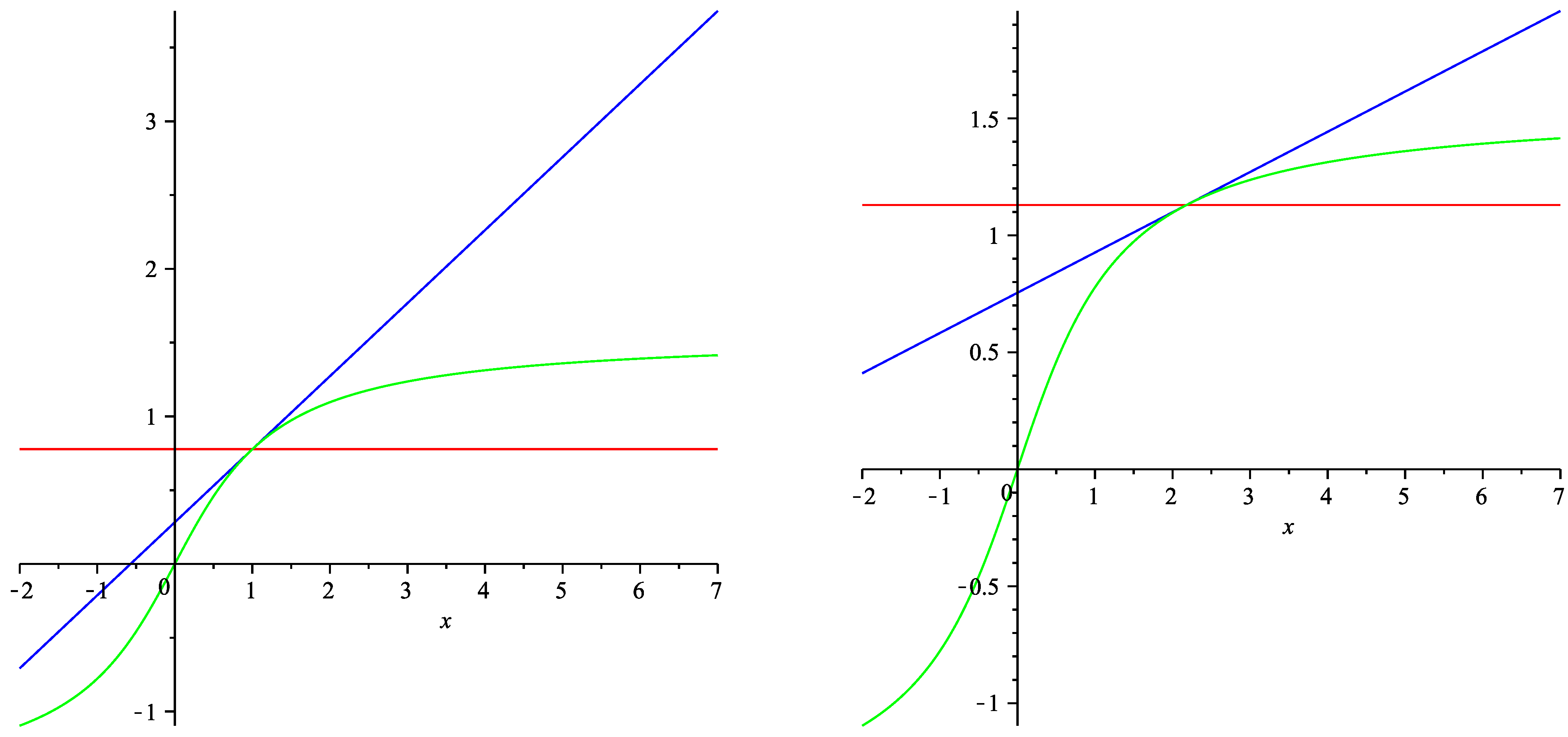
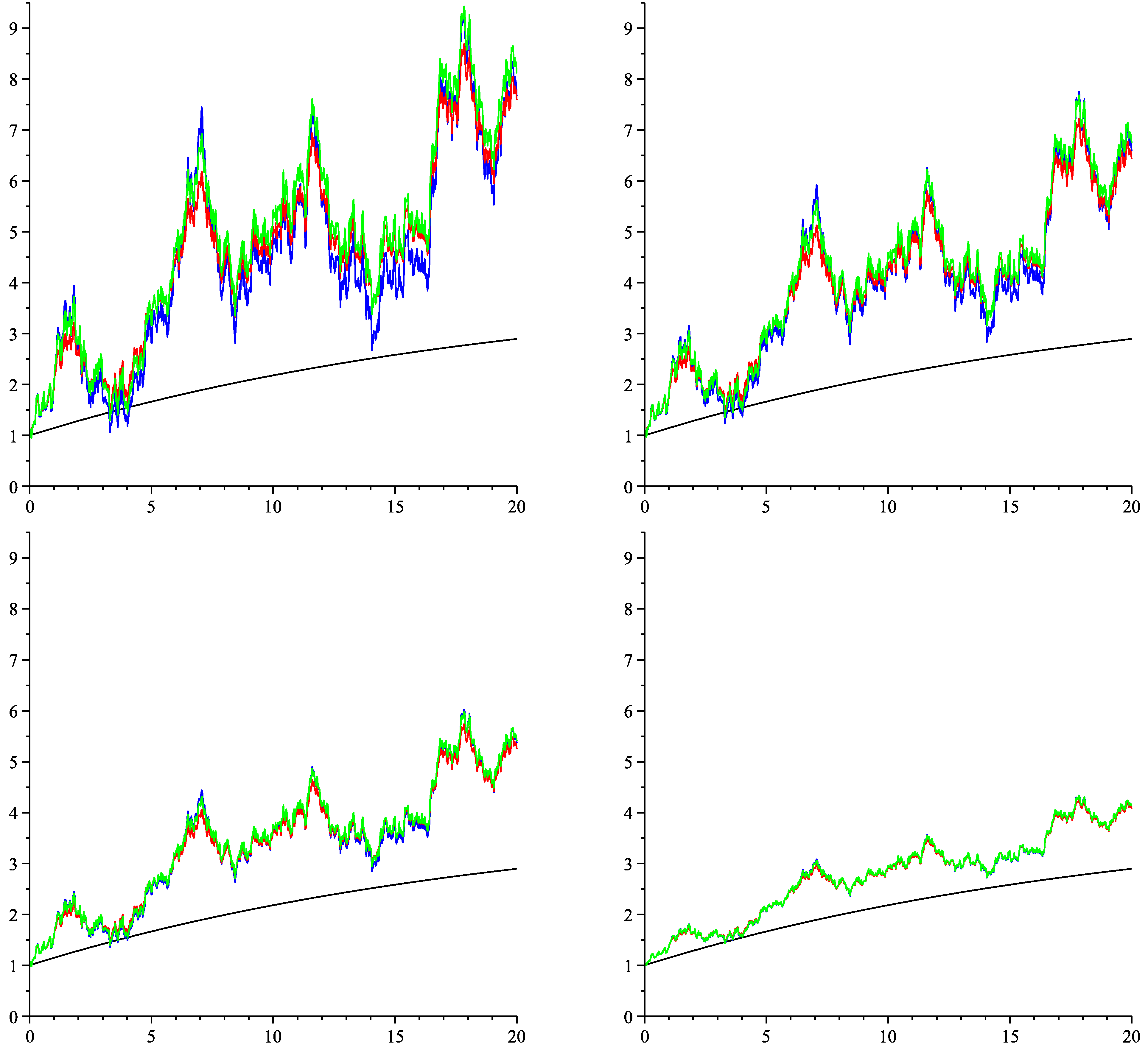
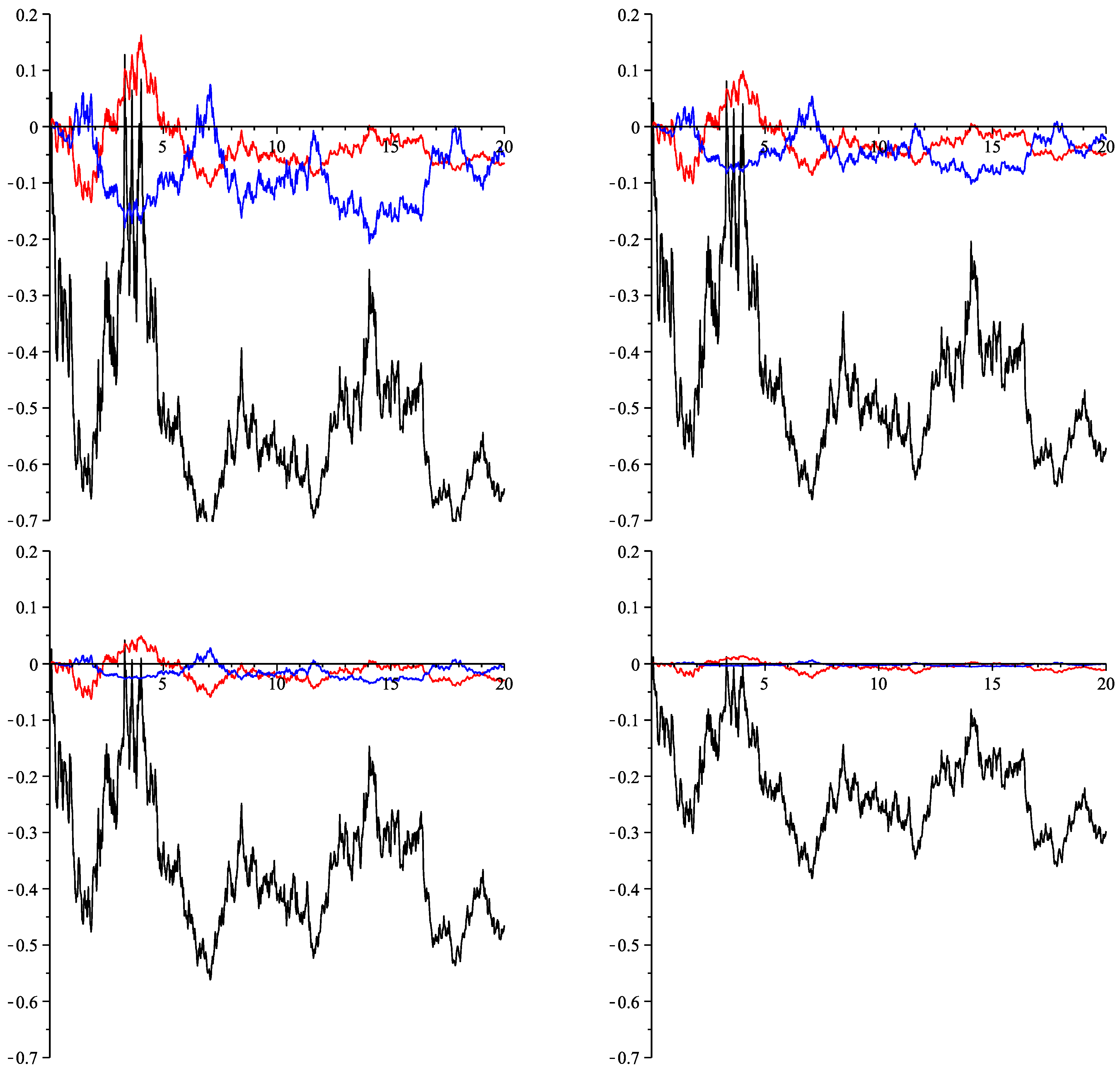
6. Numeric Illustration

We now give a numeric example that illustrates the asymptotics of the Gaussian and the affine diffusion approximation. Let X be a diffusion process that satisfies the stochastic differential equation:

$$\begin{array}{c}\hfill \text{d}X\left(t\right)=(-0.05X(t)+0.2)\text{d}t+\varsigma arctan\left(X\right(t\left)\right)\text{d}W\left(t\right),X\left(0\right)=1.\end{array}$$

(38)

Since X starts at $x_0=1$ and has a positive drift whenever $X\left(t\right)\le 4$ and ${lim}_{x\downarrow 0}\sigma (t,x)=0$, the process X is always nonnegative. The corresponding expectation function equals:

$$\begin{array}{c}\hfill E\left[X\left(t\right)\right]=4-3e^{-0.05t},t\ge 0.\end{array}$$

(39)

Figure 1. $\sigma (t,x)$ in green, $\sigma (t,E[X\left(t\right)\left]\right)$ in red and ${\sigma }^{lin}(t,x)$ in blue for $t=0$ (left) and $t=10$ (right).

Figure 1. $\sigma (t,x)$ in green, $\sigma (t,E[X\left(t\right)\left]\right)$ in red and ${\sigma }^{lin}(t,x)$ in blue for $t=0$ (left) and $t=10$ (right).

Figure 1 shows the mappings $x\mapsto \sigma (t,x)$ (green curve), $x\mapsto \sigma (t,E[X\left(t\right)\left]\right)$ (red curve) and $x\mapsto {\sigma }^{lin}(t,x)$, for $t=0$ and $t=10$. We see that $\sigma (t,E[X\left(t\right)\left]\right)$ and ${\sigma }^{lin}(t,x)$ approximate $\sigma (t,x)$ only for x close to $E\left[X\right(t\left)\right]$ quite well. Figure 2 shows a simulated path of X (green curve), the Gaussian approximation, $\tilde{X}$ (red curve) and the affine diffusion approximation $\widehat{X}$ (blue curve). For all three processes, we used the same random numbers; that is, all paths correspond to the same path of the Brownian motion, W. The smaller ς, the closer are the processes to the expectation function, $t\mapsto E\left[X\right(t\left)\right]$. Figure 3 shows the relative differences to the reference process X. Recall that the mean absolute difference between $X\left(t\right)$ and $E\left[X\right(t\left)\right]$ is of order ${\varsigma }^1$, that the mean absolute difference between $X\left(t\right)$ and $\tilde{X}\left(t\right)$ is of order ${\varsigma }^2$ and that the mean absolute difference between $X\left(t\right)$ and $\widehat{X}\left(t\right)$ is of order ${\varsigma }^3$. Indeed, $E\left[X\right(t\left)\right]$ has the greatest approximation error here. For $\varsigma =1$ and $\varsigma =0.75$, the errors of the Gaussian and the affine diffusion approximations have about the same magnitude, but for $\varsigma =0.25$, we can see a clear advantage for the affine approximation, because of its faster speed of convergence. Table 1 shows the corresponding value of:

$$\begin{array}{c}\hfill e^{-0.01{\int }_0^{20}X\left(u\right)\text{d}u}\end{array}$$

(40)

and the corresponding values of the expectation approximation, Gaussian approximation and affine approximation:

$$\begin{array}{c}\hfill e^{-0.01{\int }_0^{20}E\left[X\left(u\right)\right]\text{d}u},e^{-0.01{\int }_0^{20}\tilde{X}\left(u\right)\text{d}u},e^{-0.01{\int }_0^{20}\widehat{X}\left(u\right)\text{d}u}.\end{array}$$

(41)

The factor $0.01$ was added, because interest and mortality rates typically have magnitudes that are in the percent range. The expectation approximation clearly produces the greatest error for all sizes of ς. Interestingly, already for $\varsigma =0.75$, the error of the Gaussian and the affine approximation is quite small. As predicted by the theorems in the previous sections, the smaller ς, the more does the faster convergence speed of $\widehat{X}$ prevail and the greater is indeed the advantage of the affine approximation.

Figure 2. Expectation function $E\left[X\right(t\left)\right]$ (black) and simulated paths of $X\left(t\right)$ (green), $\tilde{X}\left(t\right)$ (red) and $\widehat{X}\left(t\right)$ (blue) for $\varsigma =1$ (top left), $\varsigma =0.75$ (top right), $\varsigma =0.5$ (bottom left), $\varsigma =0.25$ (bottom right).

Figure 2. Expectation function $E\left[X\right(t\left)\right]$ (black) and simulated paths of $X\left(t\right)$ (green), $\tilde{X}\left(t\right)$ (red) and $\widehat{X}\left(t\right)$ (blue) for $\varsigma =1$ (top left), $\varsigma =0.75$ (top right), $\varsigma =0.5$ (bottom left), $\varsigma =0.25$ (bottom right).

Table 2 shows Monte Carlo simulations for the expectations of (40) and (41) and for the mean absolute deviation of (41) from (40). We used 10,000 simulations. The affine approximation has the smallest mean absolute deviations, followed by the Gaussian approximation. This conforms with our theoretical results from the previous section. Already for $\varsigma =0.75$ the Gaussian and the affine approximation for the expectation of (40) work quite well. Surprisingly, for $\varsigma =0.5,0.25$ the Gaussian approximation seems to be closer to the true value than the affine approximation, but that may well be a random effect from the Monte Carlo simulation.

Figure 3. Relative difference of $E\left[X\right(t\left)\right]$ (black), $\tilde{X}\left(t\right)$ (red) and $\widehat{X}\left(t\right)$ (blue) with respect to $X\left(t\right)$ for $\varsigma =1$ (top left), $\varsigma =0.75$ (top right), $\varsigma =0.5$ (bottom left), $\varsigma =0.25$ (bottom right).

Figure 3. Relative difference of $E\left[X\right(t\left)\right]$ (black), $\tilde{X}\left(t\right)$ (red) and $\widehat{X}\left(t\right)$ (blue) with respect to $X\left(t\right)$ for $\varsigma =1$ (top left), $\varsigma =0.75$ (top right), $\varsigma =0.5$ (bottom left), $\varsigma =0.25$ (bottom right).

Table 1. One-path simulation for (40) and its corresponding expectation approximation, Gaussian approximation and affine approximation.

Valuation w.r.t. the Single Simulated Path	$\varsigma =1$	$\varsigma =0.75$	$\varsigma =0.5$	$\varsigma =0.25$
true value	0.37988	0.43749	0.50274	0.57575
expectation approximation	0.65644	0.65644	0.65644	0.65644
(relative error)	0.72804	0.50046	0.30573	0.14016
Gaussian approximation	0.39773	0.44968	0.50926	0.57768
(relative error)	0.04700	0.02785	0.01296	0.00336
affine approximation	0.41127	0.45185	0.50731	0.57635
(relative error)	0.08264	0.03283	0.00910	0.00105

Table 1. One-path simulation for (40) and its corresponding expectation approximation, Gaussian approximation and affine approximation.

Valuation w.r.t. the Single Simulated Path	$\varsigma =1$	$\varsigma =0.75$	$\varsigma =0.5$	$\varsigma =0.25$
true value	0.37988	0.43749	0.50274	0.57575
expectation approximation	0.65644	0.65644	0.65644	0.65644
(relative error)	0.72804	0.50046	0.30573	0.14016
Gaussian approximation	0.39773	0.44968	0.50926	0.57768
(relative error)	0.04700	0.02785	0.01296	0.00336
affine approximation	0.41127	0.45185	0.50731	0.57635
(relative error)	0.08264	0.03283	0.00910	0.00105

Table 2. Monte Carlo simulation for the expectations of (40) and (41) and for the mean absolute deviation of (41) from (40).

Valuation w.r.t. 10,000 Simulations	$\varsigma =1$	$\varsigma =0.75$	$\varsigma =0.5$	$\varsigma =0.25$
true value	0.68733	0.67571	0.66712	0.65827
expectation approximation	0.65644	0.65644	0.65644	0.65644
(mean absolute deviation)	0.16151	0.13076	0.09186	0.04839
Gaussian approximation	0.70483	0.68155	0.66873	0.65835
(mean absolute deviation)	0.10065	0.05486	0.02272	0.00500
linear noise approximation	0.70280	0.68152	0.66875	0.65839
(mean absolute deviation)	0.04802	0.02486	0.00863	0.00113

Table 2. Monte Carlo simulation for the expectations of (40) and (41) and for the mean absolute deviation of (41) from (40).

Valuation w.r.t. 10,000 Simulations	$\varsigma =1$	$\varsigma =0.75$	$\varsigma =0.5$	$\varsigma =0.25$
true value	0.68733	0.67571	0.66712	0.65827
expectation approximation	0.65644	0.65644	0.65644	0.65644
(mean absolute deviation)	0.16151	0.13076	0.09186	0.04839
Gaussian approximation	0.70483	0.68155	0.66873	0.65835
(mean absolute deviation)	0.10065	0.05486	0.02272	0.00500
linear noise approximation	0.70280	0.68152	0.66875	0.65839
(mean absolute deviation)	0.04802	0.02486	0.00863	0.00113

7. Proofs

Proof of Theorem 3.2. For a shorter notation, define:

$$\begin{array}{c}\hfill E_t^{k,l}:=\mathbb{\text{E}}\left[|X\left(t\right)-\tilde{X}{\left(t\right)|}^k{|X\left(t\right)-E\left[X\left(t\right)\right]|}^l\right]\end{array}$$

(42)

and ${\overline{X}}_t:=E\left[X\left(t\right)\right]$. The twice continuously differentiable function:

$$\begin{array}{c}\hfill g_{\epsilon }:\mathbb{\text{R}}\to (0,\infty ),x\mapsto \left\{\begin{array}{cc}|x|\hfill & \mathrm{for}|x|\ge \epsilon \hfill \\ -\frac{1}{8{\epsilon }^3}{x}^4+\frac{3}{4\epsilon }{x}^2+\frac{3\epsilon }{8}\hfill & \mathrm{for}|x|<\epsilon \hfill \end{array}\right.\end{array}$$

(43)

is for any $\epsilon >0$ a majorant of $x\mapsto |x|$ on $\mathbb{\text{R}}$. Thus, property (20) holds if for an $\epsilon >0$, there exists a constant, $C_{k,l,\epsilon }<\infty$, with:

$$\begin{array}{c}\hfill E_t^{k,l}\le E_t^{k,l,\epsilon }:=\mathbb{\text{E}}\left[g_{\epsilon }\left({(X\left(t\right)-\tilde{X}\left(t\right))}^k{(X\left(t\right)-\overline{X}\left(t\right))}^l\right)\right]\le C_{k,l,\epsilon }{\varsigma }^{2k+l},\forall t\in [0,\omega ].\end{array}$$

(44)

In contrast to $x\mapsto |x|$, the function $g_{\epsilon }$ is differentiable at zero, which allows us to apply Ito’s formula. We prove the theorem by induction. For $(k,l)=(0,0)$, we can choose $C_{0,0}=1$. The sequence of induction steps is tricky here. At first, induction arguments are presented; then, we explain the sequence of induction steps. In order to avoid case differentiations, we define $<z>:=max\{z,0\}$ and $E_t^{k,l}:=0$ for all $(k,l)\in {\mathbb{Z}}^2\setminus {\mathbb{\text{N}}}_0^2$. Applying Ito’s formula, we get:

$$\begin{array}{cc}& g_{\epsilon }\left({(X\left(t\right)-\tilde{X}\left(t\right))}^k{(X\left(t\right)-\overline{X}\left(t\right))}^l\right)-g_{\epsilon }\left(0\right)\hfill \end{array}$$

$$\begin{array}{cc}& ={\int }_0^t{g}_{\epsilon }^{\prime }\left({(X\left(s\right)-\tilde{X}\left(s\right))}^k{(X\left(s\right)-\overline{X}\left(s\right))}^l\right)(k+l){(X\left(s\right)-\tilde{X}\left(s\right))}^k{(X\left(s\right)-\overline{X}\left(s\right))}^l\alpha \left(s\right)\text{d}s\hfill \end{array}$$

$$\begin{array}{cc}& +\frac{1}{2}{\int }_0^t{\varsigma }^2{g}_{\epsilon }^{\prime }\left({(X\left(s\right)-\tilde{X}\left(s\right))}^k{(X\left(s\right)-\overline{X}\left(s\right))}^l\right)\hfill \end{array}$$

$$\begin{array}{cc}& \times (k(k-1){(X\left(s\right)-\tilde{X}\left(s\right))}^{<k-2>}{(X\left(s\right)-\overline{X}\left(s\right))}^l\parallel \sigma (X\left(s\right),s)-\sigma (\overline{X}\left(s\right),s){\parallel }^2\hfill \end{array}$$

$$\begin{array}{cc}& +2kl{(X\left(s\right)-\tilde{X}\left(s\right))}^{<k-1>}{(X\left(s\right)-\overline{X}\left(s\right))}^{<l-1>}\left(\sigma (X\left(s\right),s)-\sigma (\overline{X}\left(s\right),s)\right)\sigma {(X\left(s\right),s)}^T\hfill \end{array}$$

$$\begin{array}{cc}& +l(l-1){(X\left(s\right)-\tilde{X}\left(s\right))}^k{(X\left(s\right)-\overline{X}\left(s\right))}^{<l-2>}\parallel \sigma (X\left(s\right),s){\parallel }^2)\text{d}s\hfill \end{array}$$

$$\begin{array}{cc}& +\frac{1}{2}{\int }_0^t{\varsigma }^2{g}_{\epsilon }^{\prime \prime }\left({(X\left(s\right)-\tilde{X}\left(s\right))}^k{(X\left(s\right)-\overline{X}\left(s\right))}^l\right)\hfill \end{array}$$

$$\begin{array}{cc}& \times (k^2{(X\left(s\right)-\tilde{X}\left(s\right))}^{2<k-1>}{(X\left(s\right)-\overline{X}\left(s\right))}^{2l}\parallel \sigma (X\left(s\right),s)-\sigma (\overline{X}\left(s\right),s){\parallel }^2\hfill \end{array}$$

$$\begin{array}{cc}& +2kl{(X\left(s\right)-\tilde{X}\left(s\right))}^{<2k-1>}{(X\left(s\right)-\overline{X}\left(s\right))}^{<2l-1>}\left(\sigma (X\left(s\right),s)-\sigma (\overline{X}\left(s\right),s)\right)\sigma {(X\left(s\right),s)}^T\hfill \end{array}$$

$$\begin{array}{cc}& +l^2{(X\left(s\right)-\tilde{X}\left(s\right))}^{2k}{(X\left(s\right)-\overline{X}\left(s\right))}^{2<l-1>}\parallel \sigma (X\left(s\right),s){\parallel }^2)\text{d}s\hfill \end{array}$$

$$\begin{array}{cc}& +{\int }_0^t\cdots \text{d}{W}_s.\hfill \end{array}$$

(45)

Taking expectations on both sides makes the last integral zero, since its integrand is square integrable (to see that, apply Theorem 4.5.4 in [26] and Hölders inequality). Since:

• we have $-1\le g_{\epsilon }^{\prime }\left(x\right)\le 1$ and $0\le x{g}_{\epsilon }^{\prime \prime }\left(x\right)\le 3/2$ for all $x\in \mathbb{\text{R}}$,
• the continuous function, α, has a finite bound, $|\alpha \left(t\right)|\le {\alpha }_{max}$, on $[0,\omega ]$,
• the mapping, $\sigma (x,t)$, is Lipschitz-continuous in x with Lipschitz constant K,
• $\parallel \sigma (X\left(s\right),s)\parallel \le \parallel \sigma (X\left(s\right),s)-\sigma (\overline{X}\left(s\right),s)\parallel +\parallel \sigma (\overline{X}\left(s\right),s)\parallel \le K|X\left(s\right)-\overline{X}\left(s\right)|+\parallel \sigma (\overline{X}\left(s\right),s)\parallel$ for all s,
• ${\parallel \sigma (X\left(s\right),s)\parallel }^2\le 2K^2|X\left(s\right)-\overline{X}{\left(s\right)|}^2+2{\parallel \sigma (\overline{X}\left(s\right),s)\parallel }^2$ for all s,
• the continuous function $t\mapsto \parallel \sigma (\overline{X}\left(t\right),t)\parallel$ has a finite bound ${\sigma }^{max}$ on $[0,\omega ]$,

the expectation of the left-hand side has for $k\ne 1$ and $l\ne 1$ an upper bound of:

$$\begin{array}{cc}& \mathbb{\text{E}}\left[g_{\epsilon }\left({(X\left(t\right)-\tilde{X}\left(t\right))}^k{(X\left(t\right)-\overline{X}\left(t\right))}^l\right)\right]-\frac{3}{8}\epsilon \hfill \end{array}$$

$$\begin{array}{cc}& \le {\int }_0^t(k+l)E_s^{k,l}{\alpha }_{max}\text{d}s\hfill \end{array}$$

$$\begin{array}{cc}& +\frac{{\varsigma }^2}{2}{\int }_0^t(k(k-1)E_s^{k-2,l+2}{K}^2+2kl{E}_s^{k-1,l+1}{K}^2+2kl{E}_s^{k-1,l}K{\sigma }_{max}\hfill \end{array}$$

$$\begin{array}{cc}& +2l(l-1)E_s^{k,l}{K}^2+2l(l-1)E_s^{k,l-2}{\sigma }_{max}^2)\text{d}s\hfill \end{array}$$

$$\begin{array}{cc}& +\frac{{\varsigma }^2}{2}{\int }_0^t\frac{3}{2}(k^2{E}_s^{k-2,l+2}{K}^2+2kl{E}_s^{k-1,l+1}{K}^2+2kl{E}_s^{k-1,l}K{\sigma }_{max}\hfill \end{array}$$

$$\begin{array}{cc}& +2l^2{E}_s^{k,l}{K}^2+2l^2{E}_s^{k,l-2}{\sigma }_{max}^2)\text{d}s.\hfill \end{array}$$

(46)

Hence, since we assumed that $\varsigma \le 1$, we obtain:

$$\begin{array}{c}\hfill E_t^{k,l}\le E_t^{k,l,\epsilon }\le \frac{3}{8}\epsilon +{\int }_0^t\left(\text{const}{E}_s^{k,l}+\text{const}{\varsigma }^2\left(E^{k-2,l+2}+E^{k-1,l+1}+E^{k-1,l}+E^{k,l-2}\right)\right)\text{d}s.\end{array}$$

(47)

If inequality (20) holds for $\left\{\right(k-2,l+2),(k-1,l+1),(k-1,l),(k,l-2\left)\right\}$, then we can show that:

$$\begin{array}{c}\hfill E_t^{k,l}\le \frac{3}{8}\epsilon +{\int }_0^t\text{const}{E}_s^{k,l}\text{d}s+\text{const}{\varsigma }^2\left({\varsigma }^{2k-4+l+2}+{\varsigma }^{2k-2+l+1}+{\varsigma }^{2k-2+l}+{\varsigma }^{2k+l-2}\right).\end{array}$$

(48)

For $\epsilon \to 0$ and with Gronwall’s inequality (cf. Lemma 4.5.1 in [26]), we get:

$$\begin{array}{c}\hfill E_t^{k,l}\le \text{const}{\varsigma }^2\left({\varsigma }^{2k-4+l+2}+{\varsigma }^{2k-2+l+1}+{\varsigma }^{2k-2+l}+{\varsigma }^{2k+l-2}\right)\le \text{const}{\varsigma }^{2k+l}\end{array}$$

(49)

for all $(k,l)\in {\mathbb{\text{N}}}_0^2$ with $k\ne 1$ and $l\ne 1$.

Let now $k=1$ and/or $l=1$. Then, analogously to the above, but additionally using that $0\le g_{\epsilon }^{\prime \prime }\left(x\right)\le 3/\left(2\epsilon \right)$ for $x\in \mathbb{\text{R}}$, we can show that:

$$\begin{array}{cc}\hfill E_t^{k,l}\le E_t^{k,l,\epsilon }\le & \frac{3}{8}\epsilon +{\int }_0^t\text{const}{E}_s^{k,l}\text{d}s\hfill \end{array}$$

$$\begin{array}{cc}& +\text{const}{\varsigma }^2\left({\varsigma }^{2k-4+l+2}+{\varsigma }^{2k-2+l+1}+{\varsigma }^{2k-2+l}+{\varsigma }^{2k+l-2}+\frac{1}{\epsilon }{\delta }_{k1}{\varsigma }^{2l+2}+\frac{1}{\epsilon }{\delta }_{l1}{\varsigma }^{4k}\right)\hfill \end{array}$$

(50)

if inequality (20) holds for $\left\{\right(k-2,l+2),(k-1,l+1),(k-1,l),(k,l-2\left)\right\}$, where ${\delta }_{ij}$ is defined as one if i equals j and zero, else. Setting $\epsilon ={\varsigma }^{2k+l}$ and applying Gronwall’s inequality, we can conclude that:

$$\begin{array}{c}\hfill E_t^{k,l}\le \text{const}{\varsigma }^2\left({\varsigma }^{2k+l-2}+{\varsigma }^{2k+l-1}\right)\le \text{const}{\varsigma }^{2k+l}\end{array}$$

(51)

whenever $k=1$ and/or $l=1$.

By using Inequalities (49) and (51), we do the induction steps along the lines: $\left\{\right(0,0),(0,1),(0,2),...\}$, $\left\{\right(1,0),(1,1),(1,2),...\}$, $\left\{\right(2,0),(2,1),(2,2),...\}$ and so forth, which ensures that being at $(k,l)$, we already have been at $\left\{\right(k-2,l+2),(k-1,l+1),(k-1,l),(k,l-2\left)\right\}$. ☐

Proof of Theorem 4.1. The proof is completely analogous to the proof of Theorem 3.2, apart from the fact that the terms:

$$\begin{array}{cc}& \parallel \sigma (X\left(s\right),s)-\sigma (\overline{X}\left(s\right),s){\parallel }^2,\left(\sigma (X\left(s\right),s)-\sigma (\overline{X}\left(s\right),s)\right)\sigma {(X\left(s\right),s)}^T,{\parallel \sigma (X\left(t\right),t)\parallel }^2\hfill \end{array}$$

(52)

have to be substituted by the terms:

$$\begin{array}{cccc}& \parallel \sigma (X\left(t\right),t)-{\sigma }^{lin}(\widehat{X}\left(t\right),t){\parallel }^2,\hfill & \hfill (\sigma (X\left(t\right),t)-{\sigma }^{lin}(\widehat{X}\left(t\right),t)){\sigma }^{lin}{(\widehat{X}\left(t\right),t)}^T,& \parallel {\sigma }^{lin}(\widehat{X}\left(t\right),t){\parallel }^2\hfill \end{array}$$

(53)

and that the upper estimates for $\parallel \sigma (X\left(s\right),s)-\sigma (\overline{X}\left(s\right),s)\parallel$ and $\parallel \sigma \left(X\right(t),t)\parallel$ have to be replaced by the upper estimates:

$$\begin{array}{cc}\hfill \parallel \sigma (X\left(t\right),t)-{\sigma }^{lin}(\widehat{X}\left(t\right),t)\parallel & \le \parallel \sigma (X\left(t\right),t)-\sigma (\widehat{X}\left(t\right),t)\parallel +\parallel \sigma (\widehat{X}\left(t\right),t)-{\sigma }^{lin}(\widehat{X}\left(t\right),t)\parallel \hfill \end{array}$$

$$\begin{array}{cc}& \le K|X\left(t\right)-\widehat{X}\left(t\right)|+\frac{1}{2}\parallel {\partial }_{xx}\sigma (\xi \left(t\right),t)\parallel |\widehat{X}\left(t\right)-\overline{X}{\left(t\right)|}^2\hfill \end{array}$$

(54)

$$\begin{array}{cc}& \le K|X\left(t\right)-\widehat{X}\left(t\right)|+\frac{1}{2}K{|\widehat{X}\left(t\right)-\overline{X}\left(t\right)|}^2\hfill \end{array}$$

(55)

for $\xi \left(t\right)$ between $\overline{X}\left(t\right)$ and $\widehat{X}\left(t\right)$, and:

$$\begin{array}{cc}\hfill \parallel {\sigma }^{lin}(\widehat{X}\left(t\right),t)\parallel & \le \underset{s}{sup}\parallel \sigma (E\left[X\left(s\right)\right],s)\parallel +K|\widehat{X}\left(t\right)-\overline{X}\left(t\right)|\hfill \end{array}$$

(56)

since $|{\partial }_x\sigma (x,t)|\le K$, because of the Lipschitz continuity of $x\mapsto \sigma (x,t)$. Furthermore, we have to set $\epsilon ={\varsigma }^{3k+l}$ instead of $\epsilon ={\varsigma }^{2k+l}$. The order of the induction steps stays the same. ☐

Proof of Theorem 5.1. Taylor’s theorem applied on the function $x\mapsto exp\{-x\}$ yields:

$$\begin{array}{c}\hfill exp\{x_0+h\}=exp\left\{x_0\right\}\left(1+...+\frac{1}{k!}{h}^k+\frac{1}{(k+1)!}{h}^{k+1}exp\left\{\xi \right\}\right)\end{array}$$

(57)

for $k\in \mathbb{\text{N}}$ and a proper ξ between zero and h. Setting $k=0$, $x_0=-{\int }_s^{t}E\left[X\left(u\right)\right]\text{d}u$ and $x_0+h=-{\int }_s^{t}X\left(u\right)\text{d}u$, we get:

$$\begin{array}{cc}& E\left[|e^{-{\int }_s^{t}X\left(u\right)\text{d}u}-e^{-{\int }_s^{t}E\left[X\left(u\right)\right]\text{d}u}|\right]\le e^{-{\int }_s^{t}E\left[X\left(u\right)\right]\text{d}u}E\left[|e^{\xi }{\int }_s^{t}X\left(u\right)-E\left[X\left(u\right)\right]\text{d}u|\right]\hfill \end{array}$$

(58)

for ξ between zero and $-{\int }_s^{t}X\left(u\right)-E\left[X\left(u\right)\right]\text{d}u$. Since X is nonnegative, the random variable, ξ, is bounded by ${\int }_s^{t}E\left[X\left(u\right)\right]\text{d}u$. Applying Theorem 3.2, we obtain (32). Applying inequality (32) and using the fact that the continuous function $t\mapsto E\left[X\right(t\left)\right]$ is bounded on $[0,\omega ]$, inequality (34) is equivalent to having an upper bound of order ${\varsigma }^1$ for:

$$\begin{array}{cc}& E\left[|e^{-{\int }_s^{t}X\left(u\right)\text{d}u}(X\left(t\right)-E\left[X\left(t\right)\right])|\right].\hfill \end{array}$$

(59)

Since X is nonnegative, we can bound the previous term by:

$$\begin{array}{c}\hfill E\left[|X(t)-E[X\left(t\right)]|\right]\le \text{const}{\varsigma }^1.\end{array}$$

(60)

Thus, we showed inequality (34). Applying Taylor’s formula with $k=1$, we get:

$$\begin{array}{cc}& e^{-{\int }_s^{t}X\left(u\right)\text{d}u}{e}^{{\int }_s^{t}E\left[X\left(u\right)\right]\text{d}u}=1-{\int }_s^{t}X\left(u\right)-E\left[X\left(u\right)\right]\text{d}u+\frac{1}{2}{\left({\int }_s^{t}X\left(u\right)-E\left[X\left(u\right)\right]\text{d}u\right)}^2{e}^{\xi }.\hfill \end{array}$$

(61)

Analogously, we can show that:

$$\begin{array}{cc}& e^{-{\int }_s^t\tilde{X}\left(u\right)\text{d}u}{e}^{{\int }_s^{t}E\left[X\left(u\right)\right]\text{d}u}=1-{\int }_s^t\tilde{X}\left(u\right)-E\left[X\left(u\right)\right]\text{d}u+\frac{1}{2}{\left({\int }_s^t\tilde{X}\left(u\right)-E\left[X\left(u\right)\right]\text{d}u\right)}^2{e}^{\tilde{\xi }}\hfill \end{array}$$

(62)

for $\tilde{\xi }$ not greater than the absolute of ${\int }_s^t\tilde{X}\left(u\right)-E\left[X\left(u\right)\right]\text{d}u$. Taking the difference of the two equations, we obtain:

$$\begin{array}{cc}& E\left[|e^{-{\int }_s^{t}X\left(u\right)\text{d}u}-e^{-{\int }_s^t\tilde{X}\left(u\right)\text{d}u}|\right]e^{{\int }_s^{t}E\left[X\left(u\right)\right]\text{d}u}\hfill \end{array}$$

$$\begin{array}{cc}& \le {\int }_s^{t}E[|X\left(u\right)-\tilde{X}\left(u\right)|]\text{d}u+\frac{1}{2}E\left[{\left({\int }_s^{t}X\left(u\right)-E\left[X\left(u\right)\right]\text{d}u\right)}^2{e}^{\xi }\right]\hfill \end{array}$$

$$\begin{array}{cc}& +\frac{1}{2}E\left[{\left({\int }_s^t\tilde{X}\left(u\right)-E\left[X\left(u\right)\right]\text{d}u\right)}^2{e}^{\tilde{\xi }}\right].\hfill \end{array}$$

(63)

According to Theorem 3.2, the first addend on the right-hand side is of order ${\varsigma }^2$. Since $exp\left\{\xi \right\}$ has a deterministic upper bound and:

$$\begin{array}{cc}\hfill E\left[{\left({\int }_s^{t}X\left(u\right)-E\left[X\left(u\right)\right]\text{d}u\right)}^2\right]& ={\int }_s^t{\int }_s^t\mathbb{C}ov(X\left(u\right),X\left(v\right))\text{d}u\text{d}v\hfill \end{array}$$

(64)

$$\begin{array}{cc}& \le {\int }_s^t{\int }_s^t\sqrt{\mathbb{V}ar\left(X\right(u\left)\right)}\sqrt{\mathbb{V}ar\left(X\right(v\left)\right)}\text{d}u\text{d}v\hfill \end{array}$$

(65)

$$\begin{array}{cc}& \le \text{const}{\varsigma }^2.\hfill \end{array}$$

(66)

The second addend on the right-hand side of inequality (63) is also of order ${\varsigma }^2$. Using Hölder’s inequality, the third addend on the right-hand side of inequality (63) has an upper bound of:

$$\begin{array}{cc}& {\left(E\left[e^{2\tilde{\xi }}\right]\right)}^{1/2}{\left(E\left[{\left({\int }_s^t\tilde{X}\left(u\right)-E\left[X\left(u\right)\right]\text{d}u\right)}^4\right]\right)}^{1/2}\hfill \end{array}$$

$$\begin{array}{cc}& \le \text{const}{\left({\int }_s^t{\int }_s^t{\int }_s^t{\int }_s^t\left(E\right[|\tilde{X}\left(u_1\right)-E\left[X\left(u_1\right)\right]{|}^4{\left]\right)}^{1/4}...\left(E\right[|\tilde{X}\left(u_4\right)-E\left[X\left(u_4\right)\right]{|}^4{\left]\right)}^{1/4}\text{d}{u}_1...\text{d}{u}_4\right)}^{1/2}\hfill \end{array}$$

(67)

$$\begin{array}{cc}& \le \text{const}{\varsigma }^2\hfill \end{array}$$

(68)

because of Theorem 4.1. Note that $E[exp\left\{2\tilde{\xi }\right\}]$ has a finite upper bound, since the absolute of ξ is bounded by the absolute of ${\int }_s^t\tilde{X}\left(u\right)-E\left[X\left(u\right)\right]\text{d}u$, where the latter term has a normal distribution, as the process $\tilde{X}$ has a stochastic differential equation with additive noise. Hence, inequality (33) holds. Applying inequality (33) yields that inequality (35) is equivalent to having an upper bound of order ${\varsigma }^2$ for:

$$\begin{array}{cc}& E\left[|e^{-{\int }_s^{t}X\left(u\right)-E\left[X\left(u\right)\right]\text{d}u}\left(X\left(t\right)-E\left[X\right(t\left)\right]\right)-e^{-{\int }_s^t\tilde{X}\left(u\right)-E\left[X\left(u\right)\right]\text{d}u}\left(\tilde{X}\left(t\right)-E\left[X\left(t\right)\right]\right)|\right].\hfill \end{array}$$

(69)

With Taylor’s approximation for $k=0$, the previous term has an upper bound of:

$$\begin{array}{cc}& E\left[|X\left(t\right)-E\left[X\left(t\right)\right]||{\int }_s^{t}X\left(u\right)-E\left[X\left(u\right)\right]\text{d}u|e^{\xi }\right]\hfill \end{array}$$

$$\begin{array}{cc}& +E\left[|\tilde{X}\left(t\right)-E\left[X\left(t\right)\right]||{\int }_s^t\tilde{X}\left(u\right)-E\left[X\left(u\right)\right]\text{d}u|e^{\tilde{\xi }}\right].\hfill \end{array}$$

(70)

Using the fact that $exp\left\{\xi \right\}$ has a deterministic upper bound and by applying Hölder’s inequality, the first addend has an upper bound of:

$$\begin{array}{cc}& {\left(E\left[|X\left(t\right)-E\left[X\left(t\right)\right]{|}^2\right]\right)}^{1/2}{\left(E\left[{\left({\int }_s^{t}X\left(u\right)-E\left[X\left(u\right)\right]\text{d}u\right)}^2\right]\right)}^{1/2}\text{const}\hfill \end{array}$$

$$\begin{array}{cc}& \le {\left(\text{const}{\varsigma }^2\right)}^{1/2}{\left(\text{const}{\varsigma }^2\right)}^{1/2}\text{const}\hfill \end{array}$$

(71)

and the second addend has an upper bound of:

$$\begin{array}{cc}& {\left(E\left[|\tilde{X}\left(t\right)-E\left[X\left(t\right)\right]{|}^3\right]\right)}^{1/3}{\left(E\left[{\left({\int }_s^t\tilde{X}\left(u\right)-E\left[X\left(u\right)\right]\text{d}u\right)}^3\right]\right)}^{1/3}{\left(E\left[e^{3\tilde{\xi }}\right]\right)}^{1/3}\hfill \end{array}$$

$$\begin{array}{cc}& \le \text{const}{\left(\text{const}{\varsigma }^3\right)}^{1/3}{\left(\text{const}{\varsigma }^3\right)}^{1/3}\text{const}.\hfill \end{array}$$

(72)

Thus, we showed inequality (35). Now, we look at inequality (36), which we prove analogously to inequality (33). Applying Taylor’s inequality for $k=2$, we obtain:

$$\begin{array}{c}\hfill \begin{array}{cc}& E\left[|e^{-{\int }_s^{t}X\left(u\right)\text{d}u}-e^{-{\int }_s^t\widehat{X}\left(u\right)\text{d}u}|\right]e^{{\int }_s^{t}E\left[X\left(u\right)\right]\text{d}u}\hfill \\ & \le {\int }_s^{t}E[|X\left(u\right)-\widehat{X}\left(u\right)|]\text{d}u+\frac{1}{2}E\left[|{\left({\int }_s^{t}X\left(u\right)-E\left[X\left(u\right)\right]\text{d}u\right)}^2-{\left({\int }_s^t\widehat{X}\left(u\right)-E\left[X\left(u\right)\right]\text{d}u\right)}^2|\right]\hfill \\ & +\frac{1}{6}E\left[{\left({\int }_s^{t}X\left(u\right)-E\left[X\left(u\right)\right]\text{d}u\right)}^3{e}^{\xi }\right]+\frac{1}{6}E\left[{\left({\int }_s^t\tilde{X}\left(u\right)-E\left[X\left(u\right)\right]\text{d}u\right)}^3{e}^{\widehat{\xi }}\right].\hfill \end{array}\end{array}$$

(73)

According to Theorem 3.2, the first addend on the right-hand side is of order ${\varsigma }^3$. With the help of the Binomial theorem and Hölder’s inequality, the second addend has an upper bound of:

$$\begin{array}{cc}& \frac{1}{2}E\left[|{\int }_s^{t}X\left(u\right)-\widehat{X}\left(u\right)\text{d}u||{\int }_s^{t}X\left(u\right)-E\left[X\left(u\right)\right]+\widehat{X}\left(u\right)-E\left[X\left(u\right)\right]\text{d}u|\right]\hfill \end{array}$$

$$\begin{array}{cc}& \le \frac{1}{2}{\left(E\left[{\left({\int }_s^{t}X\left(u\right)-\widehat{X}\left(u\right)\text{d}u\right)}^2\right]\right)}^{1/2}{\left(E\left[{\left({\int }_s^{t}X\left(u\right)-E\left[X\left(u\right)\right]+\widehat{X}\left(u\right)-E\left[X\left(u\right)\right]\text{d}u\right)}^2\right]\right)}^{1/2}.\hfill \end{array}$$

(74)

The first factor is of order ${\varsigma }^3$, while the second factor has a finite upper bound. Similarly to the estimates for the second and third addend on the right-hand side of inequality (63), we can show that the third and fourth addend on the right-hand side of inequality (73) have upper bounds of order ${\varsigma }^3$. Thus, we showed inequality (36). Applying inequality (36) yields that inequality (37) is equivalent to having an upper bound of order ${\varsigma }^3$ for:

$$\begin{array}{cc}& E\left[|e^{-{\int }_s^{t}X\left(u\right)-E\left[X\left(u\right)\right]\text{d}u}\left(X\left(t\right)-E\left[X\right(t\left)\right]\right)-e^{-{\int }_s^t\widehat{X}\left(u\right)-E\left[X\left(u\right)\right]\text{d}u}\left(\widehat{X}\left(t\right)-E\left[X\left(t\right)\right]\right)|\right].\hfill \end{array}$$

(75)

With Taylor’s approximation for $k=1$, the previous term has an upper bound of:

$$\begin{array}{cc}& E[|X\left(t\right)-\widehat{X}\left(t\right)|]\hfill \end{array}$$

$$\begin{array}{cc}& +E\left[|{\int }_s^{t}X\left(u\right)-E\left[X\left(u\right)\right]\text{d}u\left(X\left(t\right)-E\left[X\right(t\left)\right]\right)-{\int }_s^t\widehat{X}\left(u\right)-E\left[X\left(u\right)\right]\text{d}u\left(\widehat{X}\left(t\right)-E\left[X\left(t\right)\right]\right)|\right]\hfill \end{array}$$

$$\begin{array}{cc}& +\frac{1}{2}E\left[{\left({\int }_s^{t}X\left(u\right)-E\left[X\left(u\right)\right]\text{d}u\right)}^2|X\left(t\right)-E\left[X\left(t\right)\right]|e^{\xi }\right]\hfill \end{array}$$

$$\begin{array}{cc}& +\frac{1}{2}E\left[{\left({\int }_s^t\widehat{X}\left(u\right)-E\left[X\left(u\right)\right]\text{d}u\right)}^2|\widehat{X}\left(t\right)-E\left[X\left(t\right)\right]|e^{\widehat{\xi }}\right].\hfill \end{array}$$

(76)

The first addend is of order ${\varsigma }^3$. The second addend has an upper bound of:

$$\begin{array}{cc}& E\left[|{\int }_s^{t}X\left(u\right)-E\left[X\left(u\right)\right]\text{d}u||X\left(t\right)-\widehat{X}\left(t\right)|\right]+E\left[|{\int }_s^{t}X\left(u\right)-\widehat{X}\left(u\right)\text{d}u||X\left(t\right)-E\left[X\left(t\right)\right]|\right]\hfill \end{array}$$

(77)

which has an order of ${\varsigma }^4$. To see that, apply Hölder’s inequality, Theorem 3.2 and Theorem 4.1. The fourth and fifth addend of the term above have an order of ${\varsigma }^3$, which can be verified similarly to the estimates for the second and third addend on the right-hand side of inequality (63). ☐

8. Conclusions

Because of nice analytical features, in the actuarial literature, stochastic models for interest and mortality rates often have the form of Gaussian diffusions with an affine drift term and additive noise. The Gaussian diffusion framework is justified with the argument that it would reasonably approximate the true development of interest and mortality rates. We studied approximation errors if appropriate models for interest and mortality rates have the form of diffusions with affine drift, but a general noise term. We calculated theoretical bounds for absolute moments and valuation formulas, showing the speed of convergence. A numerical study illustrates the approximation error, confirming the theoretical results. Our results indicate that approximation errors are reasonable if the noise term is not too large. In particular, that might be the case when modeling the mortality intensity, since demographic changes of mortality typically happen slowly, but steadily.

We generalized the Gaussian diffusion approximation with additive noise by introducing an affine diffusion approximation with an affine noise term. We found that with an affine noise term instead of additive noise, the speed of convergence can be improved from ${\varsigma }^2$ to ${\varsigma }^3$. However, we lose the nice analytical features of the Gaussian approach.

All in all, we identified a large class of diffusion processes that can be well approximated by Gaussian diffusions with additive noise or by affine diffusions with affine noise terms. As a consequence, we can say that modeling interest and mortality rates by Gaussian diffusions is well justified if there is evidence that the true developments of future interest and mortality rates have the form of diffusion processes with an affine drift term and an arbitrary, but small, noise term.

In the present paper, we measured approximation quality by point-wise moment errors and by mean absolute errors for some specific insurance claims. Future research should consider also other approximation measures.

References

1. T. Björk. Arbitrage Theory in Continuous Time, 2nd ed. New York, NY, USA: Oxford University Press, 2004. [Google Scholar]
2. O. Vasicek. “An equilibrium characterization of the term structure.” J. Financ. Econ. 5 (1977): 177–188. [Google Scholar] [CrossRef]
3. J.C. Cox, J.E. Ingersoll, and S.A. Ross. “A theory of the term structure of interest rates.” Econometrica 53 (1985): 385–407. [Google Scholar] [CrossRef]
4. D. Heath, R. Jarrow, and A. Morton. “Bond pricing and the term structure of interest rates: A new methodology for contingent claims valuation.” Econometrica 60 (1992): 77–105. [Google Scholar] [CrossRef]
5. J.A. Beekman, and C.P. Fuelling. “Interest and mortality randomness in some annuities.” Insur. Math. Econ. 9 (1990): 185–196. [Google Scholar] [CrossRef]
6. J.A. Beekman, and C.P. Fuelling. “Extra randomness in certain annuity models.” Insur. Math. Econ. 10 (1991): 275–287. [Google Scholar] [CrossRef]
7. D. Dufresne. “The distribution of a perpetuity, with application to risk theory and pension funding.” Scand. Actuar. J. 1 (1990): 39–79. [Google Scholar] [CrossRef]
8. A. De Schepper, F. de Vijlder, M.J. Goovaerts, and R. Kaas. “Interest randomness in annuities certain.” Insur. Math. Econ. 11 (1992): 271–281. [Google Scholar] [CrossRef]
9. G. Parker. “Two stochastic approaches for discounting actuarial functions.” ASTIN Bull. 24 (1994): 167–181. [Google Scholar] [CrossRef]
10. R. Norberg, and C.M. Møller. “Thieles differential equation with stochastic interest of diffusion type.” Scand. Actuar. J. 1 (1996): 37–49. [Google Scholar] [CrossRef]
11. S.-A. Persson. “Stochastic interest rate in life insurance: The principle of equivalence revisited.” Scand. Actuar. J. 2 (1998): 97–112. [Google Scholar] [CrossRef]
12. M.A. Milevsky, and S.D. Promislow. “Mortality derivatives and the option to annuitise.” Insur. Math. Econ. 29 (2001): 299–318. [Google Scholar] [CrossRef]
13. M.H. Dahl. “Stochastic mortality in life insurance: market reserves and mortality-linked insurance contracts.” Insur. Math. Econ. 35 (2004): 113–136. [Google Scholar] [CrossRef]
14. E. Biffis. “Affine processes for dynamic mortality and actuarial valuations.” Insur. Math. Econ. 37 (2005): 443–468. [Google Scholar] [CrossRef]
15. L. Ballotta, and S. Haberman. “The fair valuation problem of guaranteed annuity options: The stochastic mortality environment case.” Insur. Math. Econ. 38 (2006): 195–214. [Google Scholar] [CrossRef]
16. A.J. Cairns, D. Blake, and K. Dowd. “Pricing death: Frameworks for the valuation and securitization of mortality risk.” Astin Bull. 36 (2006): 79–120. [Google Scholar] [CrossRef]
17. M. Dahl, and T. Møller. “Valuation and hedging of life insurance liabilities with systematic mortality risk.” Insur. Math. Econ. 39 (2006): 193–217. [Google Scholar] [CrossRef]
18. D.F. Schrager. “Affine stochastic mortality.” Insur. Math. Econ. 38 (2006): 81–97. [Google Scholar] [CrossRef]
19. D. Bauer, M. Börger, J. Ruß, and H.J. Zwiesler. “The volatility of mortality.” Asia-Pac. J. Risk Insur. 3 (2008): 184–211. [Google Scholar] [CrossRef]
20. V.R. Young. “Pricing life insurance under stochastic mortality via the instantaneous Sharpe ratio.” Insur. Math. Econ. 42 (2008): 691–703. [Google Scholar] [CrossRef]
21. Z. Shang, M. Goovaerts, and J. Dhaene. “A recursive approach to mortality-linked derivative pricing.” Insur. Math. Econ. 49 (2011): 240–248. [Google Scholar] [CrossRef]
22. H. Huang, M.A. Milevsky, and T.S. Salisbury. “Optimal retirement consumption with a stochastic force of mortality.” Insur. Math. Econ. 51 (2012): 282–291. [Google Scholar] [CrossRef]
23. S. Tappe, and S. Weber. “Stochastic mortality models: An infinite-dimensional approach.” Finance and Stochastics. (in press). [CrossRef]
24. M.C. Christiansen, and A. Niemeyer. “On the forward rate concept in multi-state life insurance.” Ulm, Germany: Preprint Series of the Faculty of Economics and Mathematics at the University of Ulm, 2013. [Google Scholar]
25. K.R. Miltersen, and S.A. Persson. “Is mortality dead? Stochastic forward force of mortality rate determined by no arbitrage.” In Working paper. Norway: University of Bergen, 2005. [Google Scholar]
26. P.E. Kloeden, and E. Platen. Numerical Solution of Stochastic Differential Equations. Berlin, Germany: Springer, 1992. [Google Scholar]