Catastrophe Insurance Modeled by Shot-Noise Processes

Chemnitz University of Technology, Reichenhainer Str. 41, Chemnitz 09126, Germany
Risks 2014, 2(1), 3-24; https://doi.org/10.3390/risks2010003
Submission received: 6 November 2013
/
Revised: 28 January 2014
/
Accepted: 29 January 2014
/
Published: 21 February 2014
(This article belongs to the Special Issue Application of Stochastic Processes in Insurance)
Abstract
:Shot-noise processes generalize compound Poisson processes in the following way: a jump (the shot) is followed by a decline (noise). This constitutes a useful model for insurance claims in many circumstances; claims due to natural disasters or self-exciting processes exhibit similar features. We give a general account of shot-noise processes with time-inhomogeneous drivers inspired by recent results in credit risk. Moreover, we derive a number of useful results for modeling and pricing with shot-noise processes. Besides this, we obtain some highly tractable examples and constitute a useful modeling tool for dynamic claims processes. The results can in particular be used for pricing Catastrophe Bonds (CAT bonds), a traded risk-linked security. Additionally, current results regarding the estimation of shot-noise processes are reviewed.
1. Introduction
An insurance company insures occurring claims in exchange for a regular premium. Numerous works study the determination of an optimal premium: for example, the premium should be high enough such that the ruin probability of the insurance company is sufficiently small. The claim sizes themselves are often considered to be independent and identically distributed, with arrival times being jump times from a Poisson process. A by now classical extension of this model considers renewal times, where the inter-arrival times are no longer exponential.
In this paper, we extend this set-up further and study arrival times with a random arrival rate. In particular, we will consider arrival rates having shot-noise features. This could, for example, be used to model the claims arrivals after a catastrophe in a dynamic way: many claims will be reported right after the catastrophe, such that the arrival rate in the beginning is high. Further claims will be announced later and later corresponding to a decreasing arrival rate. Shot-noise arrival rates directly model such an effect. An alternative application appears when considering claims caused by a flood or hail: they typically admit spatial patterns with a centre where the majority of the claims are located and a decreasing number of claims with increasing distance from the centre. In a life insurance context, a natural disaster, such as a tsunami also leads to a similar patterns.
The main idea we follow here is to give a new view on insurance claims processes inspired by recent results in credit risk. In particular, we propose a model with multiple claim arrivals, i.e., claims can occur at the same time. This is an important issue for catastrophe modeling and for pricing Catastrophe Bonds (CAT bonds). The size of CAT bond markets has been increasing tremendously over the last decade. Currently, it reaches an all-time high: the outstanding volume hit $19 billion dollars in October 2013 (sources: [1,2]).
Shot-noise processes are a well-known and well-studied object. Inspired by physical effects as in [3] many applications have been proposed. For further literature we refer to [4,5,6], among many others. Applications in the insurance context are given in [7] or in [8]. Shot-noise processes in credit risk are treated in [9,10].
More precisely, consider a Poisson process N and a non-decreasing function . Claims arrive according to the time-transformed process
This is the classical inhomogeneous Poisson process if is absolutely continuous. If , however, has jumps, then it might happen that whenever . This refers to the possibility of having more than one claim arrival at time t.
It turns out that can be replaced by a stochastic process, which is non-decreasing, and we will show how to incorporate shot-noise effects in here. The obtained results have a sufficient degree of generality, in particular, we will not need Markovianity of the shot-noise processes.
The structure of the paper is as follows: in Section 2, we introduce a general form of shot-noise processes and derive general results. In Section 2.1, we give the claims arrival process with a stochastic intensity process having a shot-noise structure. In Section 3, we study the pricing of catastrophe bonds while in Section 4, we discuss the estimating of shot-noise processes. In closing, Section 5 shows how to simulate shot-noise processes.
2. Claims with Stochastic Arrival Rate
We study models allowing for factor-driven dynamics by borrowing heavily from current developments in credit risk, in particular reduced form modeling, see [11] or [12] for detailed accounts. A particular interesting example will be given in terms of general shot-noise processes. We start by introducing an appropriate notion of cumulated intensity.
Consider a probability space with a filtration satisfying the usual conditions, i.e., is right-continuous and contains all -nullsets.
From a general viewpoint, non-life insurance can be described as follows: insurance claims are reported at the arrival times . An arrival time is an -stopping time, such that the available information at time t, given by , contains the precise timing of all claims occurred before t. The size of claim i is denoted by and we assume that the claim size is immediately available i.e., is -measurable for all . The aggregated claim amount process C is given by
2.1. Intensity and Cumulated Intensity
We start by revisiting some well-known facts for marked point processes. A detailed exposition of the theory of point processes and marked point processes may be found in [13], which we follow here. The sequence is a marked point process (MPP). If the claim sizes are non-zero, then there is a one-to-one correspondence between the marked point process and its dynamic representation and we will use both interchangeably. There is a further useful tool to describe C: the random measure M defined by
where denotes the Dirac-measure at the point .
By we denote the Borel σ-algebra on the real line. Fix . Then counts the number of claims whose claim size is in A and which occurred in . The process is a point process. If there exists a non-negative -progressive process ℓ such that with probability one and for all non-negative, -predictable processes Y it holds that
then ℓ is called the -intensity of M. In the following we generalize this definition to that of cumulated intensities.
First, for a point process with associated counting process we call a predictable random measure cumulated intensity measure if
for all non-negative -predictable processes Y. The non-decreasing, predictable process will be called cumulated intensity process.
Example 1. Doubly stochastic setting. Consider a non-decreasing process starting at zero and i.i.d., standard-exponentially distributed random variables , independent of . Set and define
Then takes the rôle of a cumulated intensity process. Note that in this model it is possible that , if has jumps. We will call this effect joint jumps in the claims arrival process.
On the other side, if is absolutely continuous i.e.,
the probability of joint jumps vanishes. Then ℓ is the intensity process of the point process .
Without further assumptions, given , the point process always exists, but can be explosive. Uniqueness of the distribution of the point process requires some further assumptions, in particular on the considered filtration, see [14].
Definition 1. Consider a marked point process with associated random measure M. Suppose that for each , has the cumulated intensity measure . Then is called -cumulated intensity measure of M.
The cumulated intensity measure determines the compensator in the Doob-Meyer decomposition, such that is also called compensator of M: if Y is predictable, such that
for all , the following process
is a -martingale. The compensator in the Doob-Meyer decomposition is unique, and so is the cumulated intensity measure of M. For further details see [15] Section II.1.
Example 2. Cramér-Lundberg model. Consider a Poisson process with jump times and assume that are independent and identically distributed (i.i.d.), and independent of . Then the claims process C is a compound Poisson process. Together with its canonical filtration given by where N denotes the -nullsets this model fits in our set-up.
Lundbergs exponential upper bound on the ruin probability is a classical result, see [7] Theorem 4.2.3, and ensures that if the insurer starts with a sufficiently high initial capital the ruin probability is small.
Example 3. Stochastic discounting. If the insurance company discounts the claim costs from arrival to today t, the following modification of Equation (1) is appropriate:
where is a non-negative, measurable function, for example or . Assuming non-negative interest rates implies that h is non-increasing in t. Moreover, . The process C in this case is a special shot-noise process which we will study in the following section in detail. Remarkably, [16] shows that the Lundberg estimate still holds under with non-increasing function g if the claim sizes are in a certain sense not too heavy-tailed.
2.2. Shot-Noise Processes
In this section we study a general class of shot-noise processes driven by time-inhomogeneous Poisson processes. In Section this class will build the cornerstone for our modeling of the cumulated intensity process .
Consider an inhomogeneous Poisson process N with intensity function λ and denote by its jump times. Let be random variables with values in , i.i.d. and independent of N. Then the driving process is a inhomogeneous compound Poisson process. Finally, consider a measurable function and define the process S by
Then we call S a shot-noise process. The function h is called noise-function. This definition is general enough for our purposes, but could be extended at the cost of more complicated results. For example, it is possible to include general random compensators for N or even infinity activity for the driving process. We refer to [4] or [17] for references and further literature on shot-noise processes.
If μ is the random measure associated with the marked point process , then
This representation shows that in general, S will not be a semi-martingale. In most applications, however, we will consider and the semi-martingale property in this case is simpler to study.
Example 4. If G is not of finite absolute variation, S is no longer a semi-martingale. For example, consider a Brownian motion W such that is -measurable. Letting
gives that which is not a semi-martingale (W is -measurable!).
For the following result, we denote by ν the compensator of μ and consider shot-noise processes of the form
Lemma 2. Fix and assume that for all and all . If
-a.s., then as in Equation (4) is a semi-martingale.
Proof. Under condition (5), we can apply the stochastic Fubini theorem in the general version given in Theorem IV.65 in [18]. Observe that
with a local martingale M. This is the semi-martingale representation of S and we conclude.
In the exponential case, i.e., when , we obtain and , such that
In this case, S is also a Markov process. This is, under quite weak assumptions, the only specification where a shot-noise process is Markovian.
For applications it is important to have a repertory of parametric families which can be used to estimate the shot-noise process from data. We give some specifications in the following example which lead to highly tractable models. These examples will partly be taken up in Example 10 in an integrated form.
Example 5. Parametric families. In this example we concentrate on the multiplicative structure
and give a number of useful specifications for the noise function g.
- (1)
- Regime switching: The shot at has a constant impact for a specified time length β and after β the impact jumps to a new level (regime) which could even be zero. For , letFor , the effect of the shot vanishes totally after a time period of length β.
- (2)
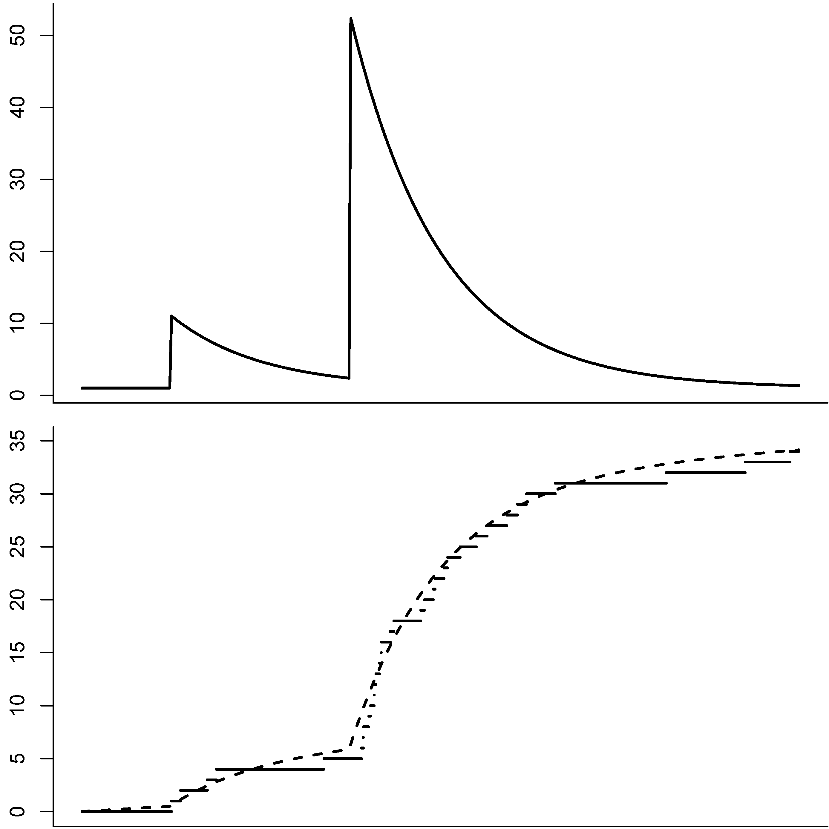
- Exponential structure: for , letHere, the effect of a shot decreases exponentially over time. As already mentioned, in this case S is Markovian. See also Figure 1 for an illustration.
We close this section with an example where claims are discounted with respect to deterministic, but non-constant interest rates.
Example 6. Discounting claims. Following Example 3 we consider claims, arriving according to a Poisson process with constant intensity ℓ. The risk-free rate of interest r is a deterministic, measurable function such that . The value of all claims arriving before T, discounted to time is given by
which is a shot-noise process with noise function Proposition 3 will enable us to compute the distribution of the discounted claims. This approach can be extended to incorporate stochastic interest rates as well.
Figure 1.
Illustration of a shot-noise process (Top) with exponential structure. The graph on the bottom shows a counting process whose jump times have the shot-noise process as intensity ℓ. The dashed line is the cumulated intensity process .
Figure 1.
Illustration of a shot-noise process (Top) with exponential structure. The graph on the bottom shows a counting process whose jump times have the shot-noise process as intensity ℓ. The dashed line is the cumulated intensity process .

Example 7. Delayed claims. Often, when a claim is announced to the insurer, the size of the claim is not known immediately. In this case, there is a delay of the claim. We could incorporate this in our set-up by letting where denotes the delay. The noise function
, allows to include such effects in multiplicative model as in Example 5.
For the description of the statistical properties of the model, the Fourier transform of the shot-noise process is a central quantity which is given in the following result. For convenience of the reader we give a proof of this classical result in our general set-up. We denote by the cumulated intensity function of the time-inhomogeneous Poisson process N.
Proposition 3. Fix and assume that for all . Let η be -distributed, independent of and
Then, for a shot-noise process S as in Equation (2) it holds for all that
The independence of and η allows to compute φ by simple integration:
In a model with multiplicative structure i.e., we have that
such that φ can be computed from the Fourier transform of . We illustrate this in Example 8 below.
Central to the proof is the following lemma which gives a relation of the jump times of the Poisson process to order statistics of i.i.d., uniformly distributed random variables. The order statistic of is obtained through ordering the sample by size, (in our case there are no ties, i.e., all values are different).
Lemma 4. Consider a (homogeneous) Poisson process N with jump times , and . Conditional on it holds that
where are i.i.d., and uniformly distributed on .
For a proof of Lemma 4 we refer to p.502 in [19].
Proof of Proposition 4. We first consider the case when . Then N is a standard Poisson process and we denote its jump times by . By Lemma 4, independence of and N, and the i.i.d. property of ξ and measurability of h we obtain that, conditionally on
Hence, as k was arbitrary it follows that
where are i.i.d., -distributed, and independent of N and ξ. Hence,
Now we utilize the representation of an inhomogeneous Poisson process as time-transformation of a standard Poisson process: the process with is a time-inhomogeneous Poisson process with intensity function λ. The jump times of are given by because
where denotes the inverse of Λ. We obtain that
and, by Equation (9),
Note that now take values in , such that . The expectation in the last equation equals
and we conclude.
Corollary 5. Assume that , such that N is a Poisson process with intensity .
- (i)
- If we obtain that is Poisson -distributed:
- (ii)
- If then S is a compound Poisson process. We denote by the Fourier transform of and obtain
- (iii)
- If we obtain the classical Markovian shot-noise process andwith
proof. The first two results follow immediately. Regarding the third claim, note that . Together with we obtain that
Then also and we obtain that
by Fubini’s theorem.
Example 8. A parametric example for the jump distribution. The following example illustrates the applicability of Proposition 3. Consider a Poisson process with intensity λ as driver and which have an Erlang distribution. This is a flexible class of positive random variables which contains the exponential and -distribution as special cases: consider with and . Then
The tractability of the Erlang-distribution mainly attributes to the following result:
We choose and compute
and we obtain the characteristic function of from Equation (10). For we obtain an exponential distribution with parameter and the obvious simplification.
2.3. Claims Driven by Shot-Noise Processes
Now we are in the position to put our ingredients together for the modeling of insurance claims. Let be a non-decreasing function denoting the cumulated claim arrival intensity when there is no shot-noise process present. As previously, we consider an inhomogeneous Poisson process N with jump times and intensity function λ. The shots are given by the i.i.d. sequence . The considered shot-noise process S is
similar to Equation (4).
As before, claims arrive at times where the associated point process has cumlated intensity measure (compensator) . In this section, the shot-noise process will be used as basis for , such that we assume that the function is non-decreasing in its first coordinate, time. Moreover, we assume that
Example 9. Shot-noise arrival rate. If the claim arrival rate ℓ is given by a shot-noise process with noise function g, then falls into the above class: note that
with . In this case, reflecting the continuity of .
As indicated in the above example we will consider integrals over shot-noise processes as cumulated intensity processes. In view of classical applications this class of processes is quite unusual as the noise function is increasing. We distinguish these two cases in our notation by always using g and G for the noise function in the original shot-noise process and the integrated shot-noise process, respectively.
For concrete implementations it is important to have a repertory of non-decreasing shot-noise processes which can be used to estimate the shot-noise process from data. We give some specifications in the following example which lead to highly tractable models.
Example 10. Parametric families. In the following examples we consider the multiplicative structure
where is non-negative and increasing in its first coordinate, and the random variables have values in .
- (1)
- Linear structure: for , letThis response function starts at α and increases linearly over the interval until it reaches 1. For , this function is absolutely continuous.
- (2)
- Exponential structure: for , letHere, G starts at α and increases exponentially to 1. The parameter α controls the impact of the jump size on S. If , G is differentiable. The parameter β controls the speed of the growth.
- (3)
- Rational structure: for , letThis provides an alternative specification to the exponential structure.
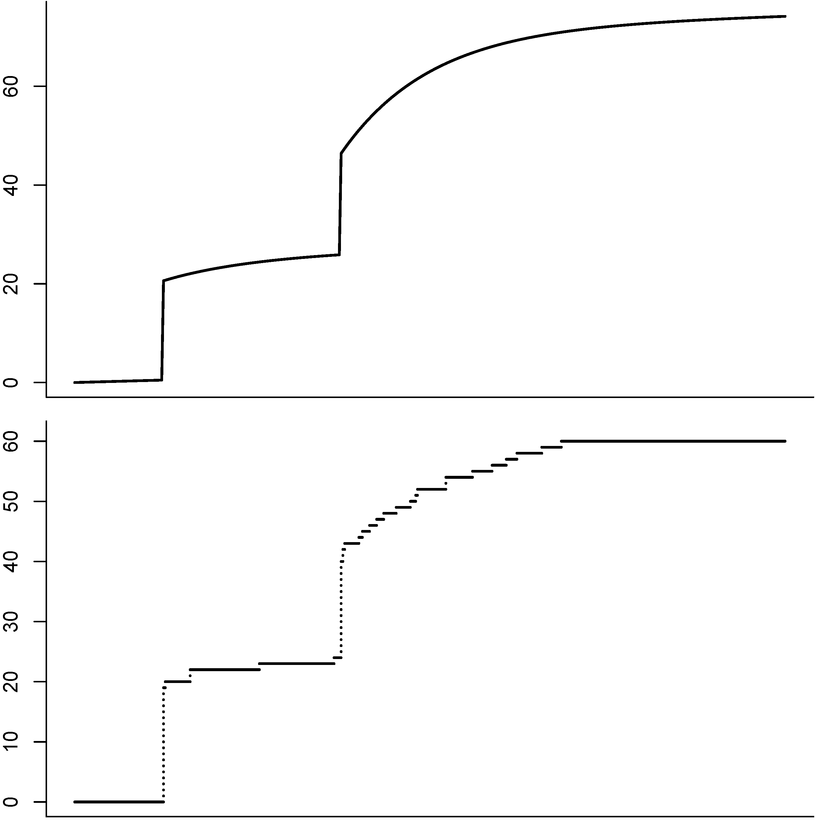
An illustration of the last example may be found in Figure 2.
Figure 2.
Illustration of the cumulated shot-noise intensity with exponential structure and jumps (). The graph on the bottom shows a counting process whose jump times have cumulated intensity process . Multiple claim arrivals occur when jumps.
Figure 2.
Illustration of the cumulated shot-noise intensity with exponential structure and jumps (). The graph on the bottom shows a counting process whose jump times have cumulated intensity process . Multiple claim arrivals occur when jumps.

3. Catastrophe Bonds
Catastrophe bonds (CAT bonds) are risk-linked securities which allow to transfer insurance risks to investors. While the valuation of car insurance can effectively be done using the law of large numbers, catastrophe risks pose a large challenge due to highly dependent claim arrivals. Our shot-noise approach sets a framework which is ideally suited to model such risks.
The size of CAT bond markets has been increasing continuously over the last decade and has reached an outstanding volume of $19 billion dollars in October 2013.
We consider the following stylized version: a CAT bond offers a coupon payment c at payment dates and the repayment of the principal 1 at if no trigger event happened. In the case of a trigger event happened, the coupons are ceased and a fraction δ of the principal is paid back.
As an example we consider as trigger event if the claims process crosses a barrier B and assume zero interest rates. In this case the payment at would be
for .
For the pricing of the CAT bond we need to choose a risk-neutral measure Q and obtain that the value of the CAT bond computes to the expectation (under Q) of discounted pay-offs i.e.,
Here is the discounting function for the time period , so for example with risk-free rate of interest r. The expectations can of course always be computed by means of a Monte-Carlo simulation. In the following, we show how to obtain a more explicit result.
First, we assume that β is deterministic. This is reasonable in insurance applications as the risks due to claims are huge in comparison to the effect of stochastic interest rates. This assumption can easily be relaxed to interest rates which are independent of the claim sizes. More general interest rate models, however, require a change of numéraire which comes at the cost of more complicated results.
If interest rates are deterministic, we obtain that
and it remains to compute the boundary crossing probabilities of the claims process in the following.
For more information on CAT bonds we refer to [22,23] or [24]. Our model also extends the approach in [8] where shot-noise Cox processes in an exponential structure with (see Example 5) have been applied to derivatives on a catastrophe index.
3.1. Equivalent Measure Changes
Following the results in [25] we study measure changes for shot-noise processes. This is an important tool for pricing, filtering as well as for importance sampling of shot-noise processes.
The basic driver of the shot-noise process S as given in Equation (2) is the marked point process . It is thus sufficient to study changes of measure for Φ. Already in [13] it was shown how to change measure as in the Girsanov theorem for marked point processes. We will present this results in the following. In [25] it was shown that these measure changes include all equivalent measure changes.
We consider an initial filtration and denote by the predictable σ-field. Denote by μ the random measure associated to Φ as in Equation (3). As above we assume that the compensator of the process is given by i.e.,
is a local martingale and the kernel is -measurable. Then is the intensity at t for a jump and, if the intensity is positive, is the respective jump-size distribution.
Consider a -measurable positive function Y such that
-almost surely and let the likelihood-process Z be given by
Fix a time horizon and assume that . Then defines a probability measure which is equivalent (as Y is positive and so Z) to . Under , Φ is a (possibly explosive) marked point process and its compensator w.r.t. is given by
3.1.1. Preserving Independent Increments
For tractability reasons one often considers shot-noise processes driven by a marked point process which has independent increments. If the increments are moreover stationary, then Φ is a Lévy process. We cover both cases in this section.
Theorem 6. Assume that . Let the density process of relative to be of the form Equation (15).
- 1.
- If Φ has independent increments under and , then Y is deterministic.
- 2.
- If Φ has independent and stationary increments under and , then Y is deterministic and does not depend on time.
Example 11. The Esscher measure. Consider a generic n-dimensional stochastic process X. Then the Esscher measure ([26]) is given by the density
where is chosen in such a way that Z is a martingale. [27] showed that the Esscher measure preserves the Lévy property. [8] applied the Esscher measure to obtain an arbitrage-free pricing methodology for catastrophe bonds under shot-noise processes.
Example 12. The minimal martingale measure. The minimal martingale measure as proposed in [28] for a certain class of shot-noise processes has been analysed in [17]. It can be described as follows: consider the semi-martingale where A is an increasing process of bounded variation and M is a local martingale. Assume that there exists a process ℓ which satisfies
Then the density of the minimal martingale measure with respect to is given by
Here denotes the Doleans-Dade stochastic exponential i.e., Z is the solution of .
In [29] the minimal martingale measure was obtained by a considering discrete time first and then taking limits.
3.2. Pricing
In [8] the authors choose the Esscher measure to obtain a pricing measure in the context of CAT bonds. Choosing the pricing measure in the case of a CAT bond is simpler than in many other cases because the underlying (the catastrophe index) is not a traded asset. In this case any equivalent measure is a martingale measure.
We take a more general approach here and only assume that certain properties of the shot-noise process hold under Q. Given this properties, we derive general pricing rules. A calibration to market data gives access to the risk-neutral measure Q. Possible ways to do this are to proceed as in [30] via Kalman filtering, or to use a minimal-distance estimation as in Section 4.
According to Theorem 6 we assume a simple structure of Φ under Q. This is in spirit with many applied results in mathematical finance, see for example [31].
- (A1) We assume that under Q the marked point process Φ has i.i.d. marks and the point process is a inhomogeneous Poisson process.
This assumption will be satisfied under an Esscher change of measure, which is an important class for insurance applications. If we have a deterministic interest rate, is constant and so for the pricing it is sufficient to compute the expectation of only.
The key to efficient pricing methodologies is to obtain the Fourier transform of the claims arrival process. In this regard, we consider the set-up as in Section 2.3: claims arrive at times where the associated point process has cumulated intensity measure (compensator) . We assume that
where is a non-decreasing measurable function. The driver of the shot-noise process is an inhomogeneous Poisson process with jump times and intensity function λ. The shots are given by the i.i.d. sequence .
Proposition 7. Consider the point process , , the independent sequence and the cumulated claims at time t,
Then, for all ,
Proof. The result follows immediately by independence as
Of course, if stems from a family of distributions which is stable under convolution, will be easy to compute. In the following result we compute the remaining probabilities.
In the doubly-stochastic case as in Example 1 we have the following, important result: recall that this setting can be viewed as a stochastic time change: , with an Poisson process with intensity 1, independent of . Then
Proposition 8. Assume that
Set
here η is -distributed, independent of . Then
Proof. We compute the right hand side of Equation (16). Consider an integrable, non-negative random variable X. Then, for all . Moreover, by monotone convergence,
and, proceeding iteratively,
Then, analogously to Proposition 3, we obtain that
and the conclusion follows.
In Example 8 the n-th derivative can be computed. Otherwise one has to resort to numerical methods.
Now the way to pricing of the CAT-bond is clear: one can either invert the Fourier transform by Fast-Fourier methods or, alternatively compute
which can sometimes be obtained explicitly, such that
4. Estimating Shot-Noise Processes
The estimation of shot-noise processes is an important part in the application of these models. A possible approach in this direction uses filtering methods and has been started in [30]. The GMM method has been applied to a special class of shot-noise processes in [32]. Further approaches for point process estimation may be found in [33] or [34]. A recent account which especially treats shot-noise processes may be found in [35] which we will present now.
The key assumption in the approach of [35] is that i.i.d. observations of the shot-noise process are at hand. The key tool to estimation is to use a parametric compensator of the point process and estimate the unknown parameter in terms of a minimum-distance estimator. In the insurance context it is often the case that i.i.d. observations are available: if used for modelling the claims arrivals after catastrophes, each catastrophe with associated claims process constitutes such a single observation.
We will consider the following case: observations consist of data of catastrophes. For each catastrophe i the claims arrive at times and we observe the point processes
on a fixed time interval . Typically will be quite large such that all claims are included in the study.
We assume that are independent and identically distributed such that each has a compensator of the same type. Each claims arrival process is driven by an individual shot-noise process in spirit of Equation (12). We assume that the time points of the catastrophes are observable: more generally, to each we associate the catastrophe arrivals which are observable. Moreover, to each there is an associated which is also assumed to be observable. It denotes a proxy for the overall size of the catastrophe. This could be obtained from expert opinions, the area of land reached by the catastrophe, or the cumulated claim sizes. It refers to the size of the shot in the compensator of .
Choosing a parametric approach, we follow Equation (12) and consider a parametric shot-noise form. More precisely, given the parameter we assume that compensator of is given by
for some .
The first step towards the estimation is the introduction of the aggregated point process and the aggregated compensator:
The second step is to define a suitable distance. For the finite measure μ we consider the semi-norm
The measure μ induced by leads to the following semi-norm
Then, the quantity
represents an overall measure of fit for the observed data to the compensator . The final estimator of is the parameter which maximizes this fit:
The following weak identifiability assumption will be needed for consistency. By we denote the closure of Θ. First, we assume that for all
- (A2) Let be a bounded open set and suppose that for eachMoreover, the process is continuous with probability one and admits a continuous extension to .
The following result, given in Theorem 1 in [35], shows consistency of the minimum-distance estimator.
Theorem 9. Assume that (A2) holds. Then
The proof of the theorem may be found in [35]. It relies on generalized U-Statistics and an appropriate version of the Hewitt-Savage 0-1 law. Under further assumptions, they also obtain asymptotic normality of the estimator and we refer to Theorem 2 in their paper for a precise statement.
This estimation procedure seems a very promising approach compared to existing methodologies and will be taken up in a future article for an estimation on insurance catastrophe data.
5. Simulation
Efficient simulation algorithms are often the key to widespread application of a model. In particular, when closed-form results are expensive or not at hand, Monte-Carlo simulation always provides an alternative which is nowadays often feasible due to available computer power. Similar to [36] we can give general simulation routines for counting processes in a doubly-stochastic setting following the methodology in [14].
Consider a fixed time horizon T. We will use the fact (see Lemma 4), that conditional on the number of jumps of a Poisson process its jump times are equal in distribution to the order statistics of i.i.d. uniform random variables on . The second key ingredient will be the time-transform: is a inhomogeneous Poisson process if is a standard Poisson process.
We shortly recall our model: is a time-inhomogeneous Poisson process with intensity function λ and jump times . The shots are i.i.d. and -valued. We denote the distribution of by . Then our shot-noise process is given by
following Equation (4). The insurance claims arrive at times which are doubly-stochastic random times with cumulated intensity process
The claim sizes itself are i.i.d. with distribution function .
Algorithm 1. Simulate one path of the shot-noise process S and, afterwards, a vector of claim arrivals together with associated claim sizes. A realized path may be found in Figure 3.
- Draw the number of jumps N from a Poisson-distribution.
- Simulate N i.i.d. U random variables and set , , being the i-th order statistic.
- Simulate N i.i.d. random variables (jump heights) according to the chosen distribution .
- Compute the path .
- Simulate the claim arrival times by taking i.i.d. exponential(1)-random variables and calculating
- Simulate the claim sizes from the distribution .
Figure 3.
Simulation of a claims process driven by a shot-noise process with rational structure. The graph shows the intensity process ℓ (Top), the cumulated intensity process (Middle) and the simulated claims process (Bottom).
Figure 3.
Simulation of a claims process driven by a shot-noise process with rational structure. The graph shows the intensity process ℓ (Top), the cumulated intensity process (Middle) and the simulated claims process (Bottom).

Conflicts of Interest
The author declares no conflicts of interest.
References
- Artemis. “Catastrophe Bond Market Hits $19 billion Outstanding for First Time.” Available online: http://www.artemis.bm/blog/2013/10/08/catastrophe-bond-market-hits-19-billion-outstanding-for-first-time/ (accessed on 17 February 2013).
- Insurance Insider. “Cat Bond Market Reaches Record $18 bn Size.” Available online: http://www.insuranceinsider.com/-1244580/8 (accessed on 17 February 2013).
- W. Schottky. “Über spontane Stromschwankungen in verschiedenen Elektrizitätsleitern.” Ann. Phys. 362 (1918): 541–567. [Google Scholar] [CrossRef]
- E. Parzen. Stochastic Processes. San Francisco, CA, USA: Holden-Day, Inc., 1962. [Google Scholar]
- R.B. Lund, R.W. Butler, and R.L. Paige. “Prediction of shot noise.” J. Appl. Probab. 36 (1999): 374–388. [Google Scholar] [CrossRef]
- C. Kühn. “Shot-noise processes.” In Encyclopedia of Actuarial Science. Chichester, UK: John Wiley & Sons, 2004, pp. 1556–1558. [Google Scholar]
- T. Mikosch. Non-Life Insurance Mathematics: An Introduction with the Poisson Process, 2nd ed. Berlin, Germany: Universitext, Springer-Verlag, 2009. [Google Scholar]
- A. Dassios, and J. Jang. “Pricing of catastrophe reinsurance & derivatives using the Cox process with shot noise intensity.” Financ. Stoch. 7 (2003): 73–95. [Google Scholar] [CrossRef] [Green Version]
- M. Scherer, L. Schmid, and T. Schmidt. “Shot-noise multivariate default models.” Eur. Actuar. J. 2 (2010): 161–186. [Google Scholar]
- J. Jang, A. Herbertsson, and T. Schmidt. “Pricing basket default swaps in a tractable shot noise model.” Stat. Probab. Lett. 8 (2011): 1196–1207. [Google Scholar]
- D. Filipović. Term Structure Models: A Graduate Course. Berlin/Heidelberg, Germany: Springer Verlag, 2009. [Google Scholar]
- T. Bielecki, and M. Rutkowski. Credit Risk: Modeling, Valuation and Hedging. Berlin/Heidelberg, Germany; New York, NY, USA: Springer Verlag, 2002. [Google Scholar]
- P. Brémaud. Point Processes and Queues. Berlin/Heidelberg, Germany; New York, NY, USA: Springer Verlag, 1981. [Google Scholar]
- J. Jacod. “Multivariate point processes: Predictable projection, Radon-Nikodym derivatives, representation of martingales.” Zeitschrift für Wahrscheinlichkeitstheorie und verwandte Gebiete 31 (1975): 235–253. [Google Scholar] [CrossRef]
- J. Jacod, and A. Shiryaev. Limit Theorems for Stochastic Processes, 2nd edn. Berlin/Heidelberg, Germany: Springer Verlag, 2003. [Google Scholar]
- P. Bremaud. “An insensitivity property of Lundberg’s estimate for delayed claims.” J. Appl. Probab. 37 (2000): 914–917. [Google Scholar] [CrossRef]
- T. Schmidt, and W. Stute. “General shot-noise processes and the minimal martingale measure.” Stat. Probab. Lett. 77 (2007): 1332–1338. [Google Scholar] [CrossRef]
- P. Protter. Stochastic Integration and Differential Equations, 2nd ed. Berlin/Heidelberg, Germany; New York, NY, USA: Springer Verlag, 2004. [Google Scholar]
- T. Rolski, H. Schmidli, V. Schmidt, and J. Teugels. Stochastic Processes for Insurance and Finance. New York, NY, USA: John Wiley & Sons, 1999. [Google Scholar]
- J. Rice. “On generalized shot noise.” Adv. Appl. Probab. 9 (1977): 553–565. [Google Scholar] [CrossRef]
- W. Smith. “Shot noise generated by a semi-Markov process.” J. Appl. Probab. 10 (1973): 685–690. [Google Scholar] [CrossRef]
- S. Cox, and H. Pederson. “Catastrophe risk bonds.” N. Am. Actuar. J. 4 (2000): 56–82. [Google Scholar]
- H. Louberge, E. Kellezi, and M. Gilli. “Using catastrophe-linked securities to diversify insurance risk: A financial analysis of CAT bonds.” J. Insur. Issues 22 (1999): 125–146. [Google Scholar]
- M. Lewis. “In Natures’ Casino.” New York Times, 26 August 2007. [Google Scholar]
- T. Schmidt. Shot-Noise Processes: Equivalent Measure Changes and Applications in Finance and Filtering. Working Paper; 2014. [Google Scholar]
- F. Esscher. “On the probability function in the collective theory of risk.” Skand. Aktuarietidskr. 15 (1932): 175–195. [Google Scholar]
- F. Esche, and M. Schweizer. “Minimal entropy preserves the Lévy property: How and why.” Stoch. Process. Appl. 115 (2005): 299–327. [Google Scholar] [CrossRef]
- H. Föllmer, and M. Schweizer. “Hedging of Contingent Claims under Incomplete Information.” In Applied Stochastic Analysis. Edited by M.H.A. Davis and R.J. Elliott. London, UK; New York, NY, USA: Gordon and Breach, 1990, Volume 5, pp. 389–414. [Google Scholar]
- T. Altmann, T. Schmidt, and W. Stute. “A shot noise model for financial assets.” Int. J. Theor. Appl. Financ. 11 (2008): 87–106. [Google Scholar] [CrossRef]
- A. Dassios, and J. Jang. “Kalman-Bucy filtering for linear systems driven by the Cox process with shot noise intensity and its application to the pricing of reinsurance contracts.” J. Appl. Probab. 42 (2005): 93–107. [Google Scholar] [CrossRef]
- R.J. Elliott, and D.B. Madan. “A discrete time extended Girsanov prinicple.” Math. Financ. 8 (1998): 127–152. [Google Scholar] [CrossRef]
- M. Moreno, P. Serrano, and W. Stute. “Statistical properties and economic implications of jump-diffusion processes with shot-noise effects.” Eur. J. Oper. Res. 214 (2011): 656–664. [Google Scholar] [CrossRef]
- M. Jacobsen. Statistical Analysis of Counting Processes: Lecture Notes in Statistics. New York, NY, USA: Springer-Verlag, 1982, Volume 12. [Google Scholar]
- A.F. Karr. Point Processes and Their Statistical Inference: Probability: Pure and Applied. New York, NY, USA: Marcel Dekker Inc., 1986, Volume 2. [Google Scholar]
- K. Kopperschmidt, and W. Stute. “The statistical analysis of self-exciting point processes.” Stast. Sinica 23 (2013): 1273–1298. [Google Scholar]
- D. Filipović, L. Overbeck, and T. Schmidt. “Dynamic CDO term structure modelling.” Math. Financ. 21 (2011): 53–71. [Google Scholar] [CrossRef]
© 2014 by the author; licensee MDPI, Basel, Switzerland. This article is an open access article distributed under the terms and conditions of the Creative Commons Attribution license (http://creativecommons.org/licenses/by/3.0/).
Share and Cite
MDPI and ACS Style
Schmidt, T. Catastrophe Insurance Modeled by Shot-Noise Processes. Risks 2014, 2, 3-24. https://doi.org/10.3390/risks2010003
AMA Style
Schmidt T. Catastrophe Insurance Modeled by Shot-Noise Processes. Risks. 2014; 2(1):3-24. https://doi.org/10.3390/risks2010003
Chicago/Turabian StyleSchmidt, Thorsten. 2014. "Catastrophe Insurance Modeled by Shot-Noise Processes" Risks 2, no. 1: 3-24. https://doi.org/10.3390/risks2010003