Modeling and Performance of Bonus-Malus Systems: Stationarity versus Age-Correction

Department of Mathematics, Aarhus University, Ny Munkegade, Aarhus C 8000, Denmark
Risks 2014, 2(1), 49-73; https://doi.org/10.3390/risks2010049
Submission received: 30 September 2013
/
Revised: 17 February 2014
/
Accepted: 18 February 2014
/
Published: 11 March 2014
(This article belongs to the Special Issue Application of Stochastic Processes in Insurance)
Abstract
:In a bonus-malus system in car insurance, the bonus class of a customer is updated from one year to the next as a function of the current class and the number of claims in the year (assumed Poisson). Thus the sequence of classes of a customer in consecutive years forms a Markov chain, and most of the literature measures performance of the system in terms of the stationary characteristics of this Markov chain. However, the rate of convergence to stationarity may be slow in comparison to the typical sojourn time of a customer in the portfolio. We suggest an age-correction to the stationary distribution and present an extensive numerical study of its effects. An important feature of the modeling is a Bayesian view, where the Poisson rate according to which claims are generated for a customer is the outcome of a random variable specific to the customer.
1. Introduction
In the classical actuarial model for bonus-malus systems in automobile insurance (Denuit et al. [1] or Lemaire [2], for example), there is a finite set of bonus classes . A customer having n claims and bonus class ℓ in a given year has bonus class in the next for some deterministic function b (the bonus rule; claim sizes are ignored and only claim numbers counted). The customer has a risk parameter λ, such that the number of claims in consecutive years are i.i.d. Poisson, and so the sequence of bonus classes is a time-homogeneous Markov chain with transition matrix where
(such a customer we denote a λ-customer). Customers pay premium when in class ℓ and enter the system in some fixed class . The and may be chosen according to certain optimality and/or financial equilibrium principles (see below) or arbitrarily.
For a simple example of a bonus rule, consider the rule. Here each claim causes the bonus level to increase by 2, whereas it decreases by 1 for each claim-free year (obvious boundary modifications apply to levels ). The systems in use are often substantially more detailed, with K of order 15–25.
Much of the discussion of the literature employs stationarity modeling, measuring characteristics of the system via the stationary distribution (existing under the weak assumptions of irreducibility and aperiodicity). In particular, the average premium of a customer with risk parameter λ is defined by
where the are the n-step transition probabilities. From the , one often proceeds to calculate the Loimaranta efficiency
at λ (denoted elasticity outside the actuarial sciences); it measures to which extent is linear at λ (as should ideally be the case), with expressing ‘local linearity’ at λ.
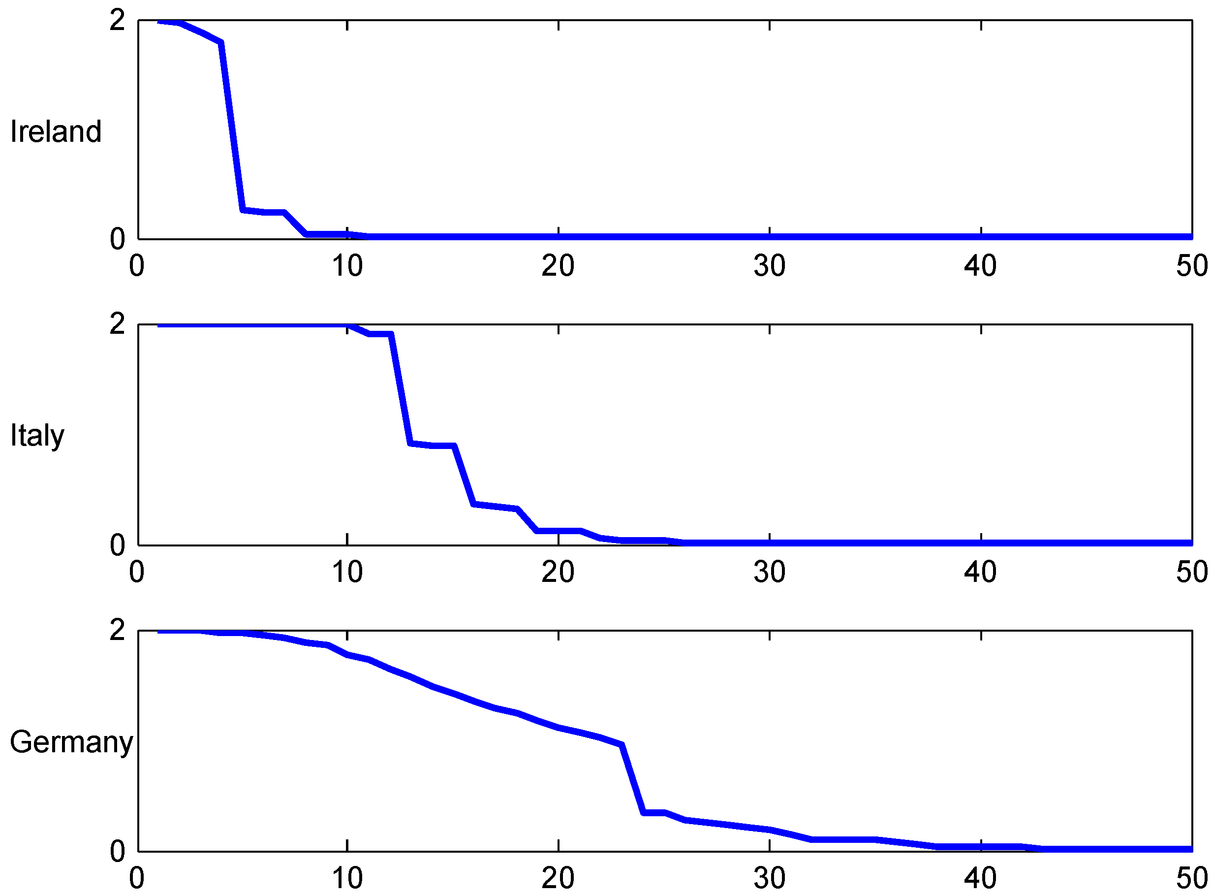
Such stationary performance measures are only meaningful if the Markov chain L attains (approximate) stationarity within the typical time a customer spends in the portfolio. For this reason much attention has been given to studying the approach of the to . The rate of convergence is known to be geometric, with decay parameter the second largest eigenvalue of the transition matrix . However, this is an asymptotic result and so the studies are most often numerical, depicting for example the mean annual premium or the total variation (t.v.) distance
as function of n (see, for example, Denuit et al. [1], p. 183ff). The results are sometimes encouraging: for some bonus systems, already for 4–6. However, these are typically simple-minded systems, and for the more realistic ones, one often sees a substantial value of the t.v. distance for say , a value exceeding the time span a customer can be expected to stay in the portfolio. Nevertheless, the studies of the effects of the sojourn time A in the portfolio being finite are remarkably few, with Borgan et al. [3] being the main exception. One purpose of this paper is to go deeper into this direction and to formulate an alternative (which we call age-correction) to the stationarity point of view.
Bonus-malus systems may be seen as an example of experience rating which has as aim to calculate the premium on an individual basis by using the information available to the company. In the automobile insurance setting, we ignore in this paper profit, administration costs etc., and take the average claim size equal to 1, so that in after a given year m, the company would want to compute its net premium for year m as its best guess of the customer’s λ as function of the numbers of claims filed in years . The naive guess is of course the average . However, a high value of could be due to bad luck of an otherwise good driver and a low value luck of an otherwise bad driver. An estimate which is more fair to the customer is therefore obtained by a Bayesian view where one involves information on the population of customers in form of a prior distribution, say U, of λ, views the particular customer’s λ as the outcome of a r.v. with distribution U, calculates the posterior distribution and takes as the mean of , the Bayes premium.
Example 1. A often considered choice for the prior U is a Gamma with density . This can be motivated by negative binomial fitting (e.g., Denuit et al. [1], p. 28), but is also mathematically convenient since then the posterior is again Gamma with parameters
and one gets the Bayes premium as the posterior mean
This has a neat interpretation as a weighted average of the population mean (the premium the company will charge without access to claims statistics) and the mean of the claims, with the weight of increasing to 1 as years go by and the information on the customer accumulates. ☐
The Bayes premium enjoys the optimality property of minimizing the quadratic loss in the class of all functions of , the natural class of predictors of Λ using information on . In fact, it is standard that the solution to this minimization problem is . For these facts and the general theory of Bayes premiums, see Bühlmann [4], Bühlmann & Gisler [5] and Denuit et al. ([1], Ch. 3). 1
Given the above optimality property, the Bayes premium can be viewed as the optimal fair choice of the insurer’s premium (it is often argued that the reason that bonus-malus systems are used instead in practice is that they are better understandable to the average customer who would not know about prior and posterior distributions). Nevertheless, as noted by Norberg [6], the Bayesian view is highly relevant also in bonus-malus systems but for a different purpose, to compute the premiums in the different bonus levels. To this end, the idea of basing the premium on the bonus level means that one chooses the minimizer of in the class of all functions c of the bonus level. One then needs to specify what is meant by this level, and to avoid the dependency on m, the choice of [6] and much subsequent literature is a r.v. distributed as (recall that is the stationary distribution of the Markov chain when the customer’s Poisson parameter is λ). Using the general -theory quoted above, the minimizer is
so that the optimal bonus level in class ℓ is . Evaluating the conditional expectation, we get
Formula (3) gives the premium rule of the bonus system which is optimal from the point of view of minimizing the error in predicting a customer’s Λ. 2
The rule (3) enjoys in a certain sense the principle of financial equilibrium (for the company) which asserts that on average, premium incomes and payments of claims should balance. Namely, the expected claims in a year of a typical customer is and his expected premiums are assuming that a typical customers bonus class is distributed as the stationary r.v. . By the tower property of conditional expectations, these expressions coincide. However, the point we take in this paper is that this assumption is questionable and needs further discussion.
Remark 1. The above set-up ignores claim amounts (for examples of discussion involving also claim severity, see Frangos & Vontos [7] and Mahmoudvand & Hassani [8]). For simplicity, we will assume that the monetary scale is chosen such that the mean claim size is one. ☐
Remark 2. Regulations vary greatly from country to country. At one extreme, all insurance companies are obliged to use the same bonus-malus system, at the other they have complete freedom. The general tendency has gone towards deregulation. A detailed survey of the situation in Europe as of year 2000 concerning such rules is in Meyer [9]. Of course, much has changed since then but still, [9] will serve to give an impression of many practical issues connected with motor insurance. ☐
The paper is organized as follows. In Section 2, we introduce our age-correction approach and give some of its simple properties. The fundamental formula (4) gives , the age-corrected π, expressed in terms of the sojourn distribution of a customer in the population. Section 3, Section 4, Section 5 and Section 6 then contain an extensive numerical study of its behavior in concrete case and how it compares to the traditional stationarity-based approach. A concluding discussion, including more careful references to the literature, is in Section 7, and the Appendix contains some complements as well as an outline of a more general modeling approach via Markov chains.
2. Independent Sojourn Times
Motivated by the criticism of the traditional use of stationarity, we now assume that a customer stays in the portfolio only for a finite number of years A. i.e., he is in the portfolio in years after entering. We further assume that A is independent of his Λ and his claim sequence and thereby his sequence of bonus levels, and that . This independence assumption is crucial but of course questionable. For example, an insured with a high Λ will typically be in a high bonus class and be more prone to change company than one with a small Λ. The distribution of A is denoted by F, the point probabilities by , and we write , . Here is the equilibrium distribution familiar from renewal theory, cf. ([10], V.3). It gives the distribution of the time elapsed since the last renewal, an interpretation that matches nicely the alternative derivation we give in Appendix B.
Much of the discussion of Section 1 remains relevant, only do we need for each value λ of the Poisson parameter to replace the stationary distribution of the bonus level by the distribution of the typical bonus level .
We then need to specify what is meant by the ‘typical bonus level’ of a λ-customer, and our suggestion is to define this as a r.v. with distribution
denoted the age-corrected distribution in the rest of the paper. Expression (4) is fundamental for the paper and may be approached in various ways. We choose here the set-up in the following Theorem 1 where the interpretation is as a limiting long-term average of bonus classes of λ-customers seen by the company (for an alternative, see Appendix B).
Before stating the Theorem, we need some notation and assumptions. Let denote the number of λ-customers in the portfolio in year , the number of λ-customers entering the portfolio 3 4 and , the bonus classes of the λ-customers, the time since they entered the portfolio. Assume that the are i.i.d. with finite mean and independent of the with , and that the for different customers are i.i.d. and independent of the .
Theorem 1. Under the above assumptions,
a.s. as for all ℓ, no matter initial conditions.
Proof. We can write
where is the time-in-portfolio-before-Y of λ-customers that first entered the portfolio at some time , the similar time of those that entered at some time and left before , and the time of those that entered at some time but still remain in the portfolio at time (and possibly after). Here we can bound by , the total-time-in-portfolio (not necessarily before Y) of λ-customers that first entered at some time but remained in the portfolio after Y. By the law of large numbers, . Further,
Combining these facts gives
A similar argument shows that the total times or λ-customers ever spend is bonus class ℓ (not necessarily before Y) is of order
and that the contribution to the l.h.s. of (6) dominates the and contributions. Combining with (7) gives (6). The proof of (5) is similar, though slightly easier. ☐
Remark 3. The analysis in the proof of Theorem 1 is similar to the one of a discrete time G/G/∞ queue. then plays the role of the queue length at time y, and as the elapsed service time of customer . We will not use this connection and hence leave out further details. ☐
It may be noted that expression (4) may be evaluated in closed analytical form. To this end, we need the fundamental matrix of the Markov chain given by where is the (row) vector with 1 at all entries ([10], p. 31). Further let denote p.g.f. of F and use the same notation for a square matrix . Then, with the ℓth (row) unit vector:
Theorem 2. The distribution with point probabilities (4) is given by
For the proof, see the Appendix.
Remark 4. If the univariate p.g.f. is available in closed form, then so is usually the matrix version by obvious changes in the expression for . For example for a negative binomial distribution of order 2 with point probabilities , , we have and .
3. Numerical Set-up
3.1. The Bonus Systems
We have selected three rather different systems for our numerical studies. Doing so, our source has been the survey in Meyer [9] treating the situation in most European countries (as well as Japan and the US) around 1999. Important characteristics of a bonus system is the number K of classes and the spread factor, defined as the ratio between the highest premium and the lowest . We chose systems from three countries, Ireland, Italy and Germany. Ireland has a small number of classes and a low spread factor of 2, Germany has a high number of classes and a high spread factor of 8.2, whereas Italy is intermediate with of classes and spread factor 4. More detail on the various systems are given below. It should be noted that each system may only have been one among several in the particular country when [9] was published and that much may have changed since then. However, our point is not to analyze systems that are necessarily in current use but rather that our examples both show diversity and are typical of many other systems.
The premiums , often called relativities, are traditionally given in percent of the premium in the initial class or some other reference class, and when presenting the three systems, we follow that tradition (as does Meyer [9]). However, later we shall renormalize to get financial equilibrium.
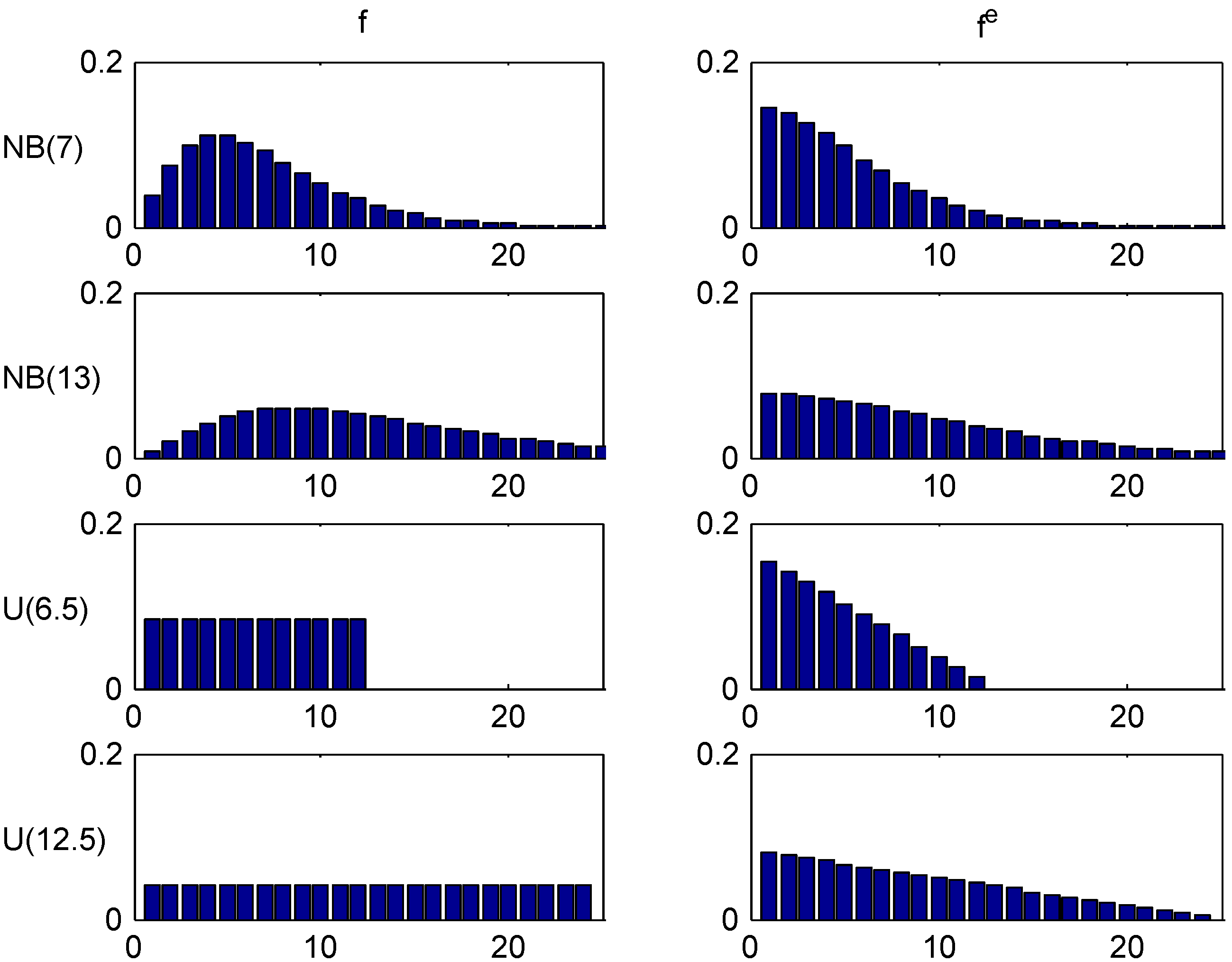
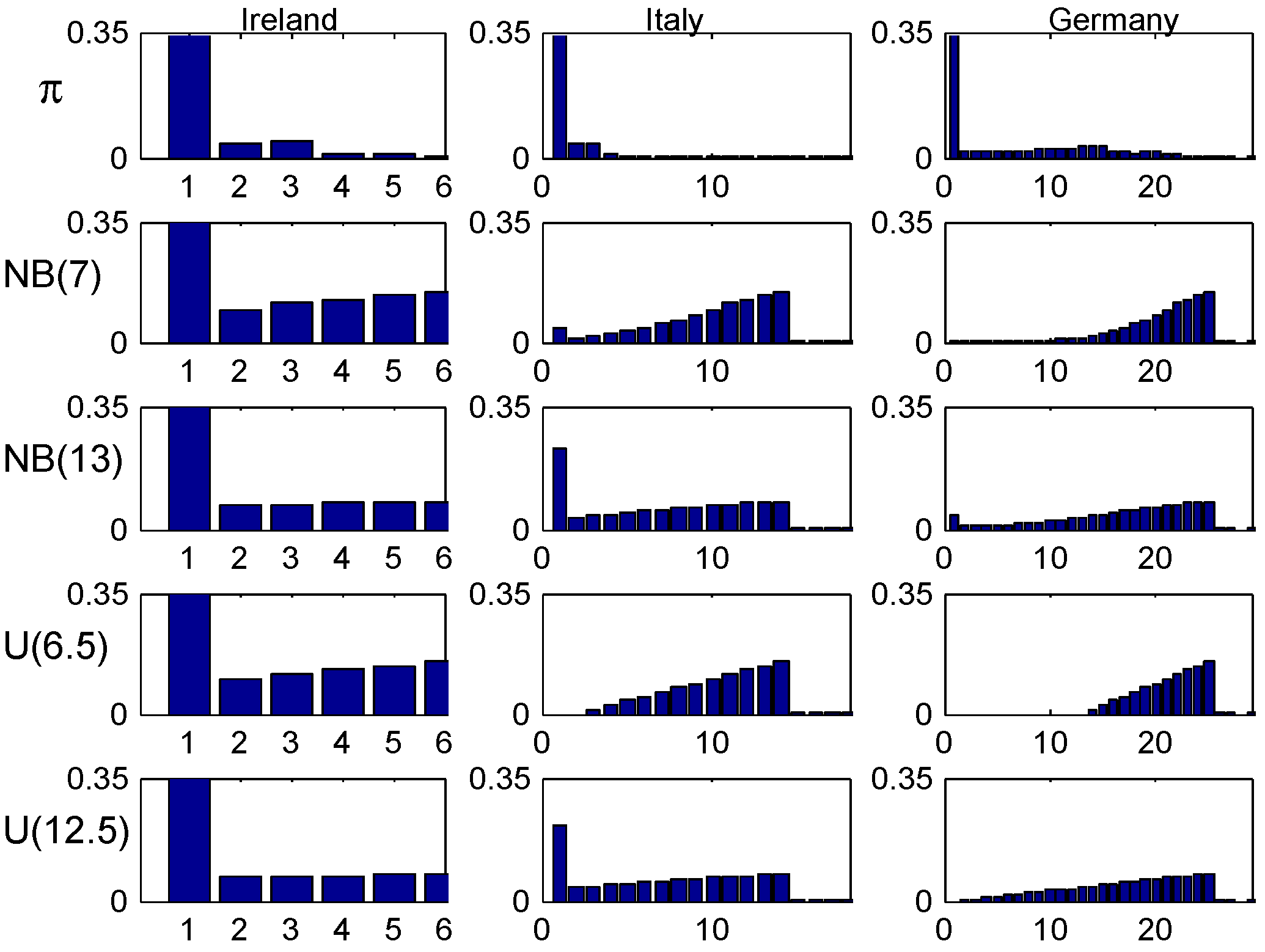
Figure 1.
Trial distributions and their equilibrium distributions.

3.2. Trial Sojourn Time Distributions
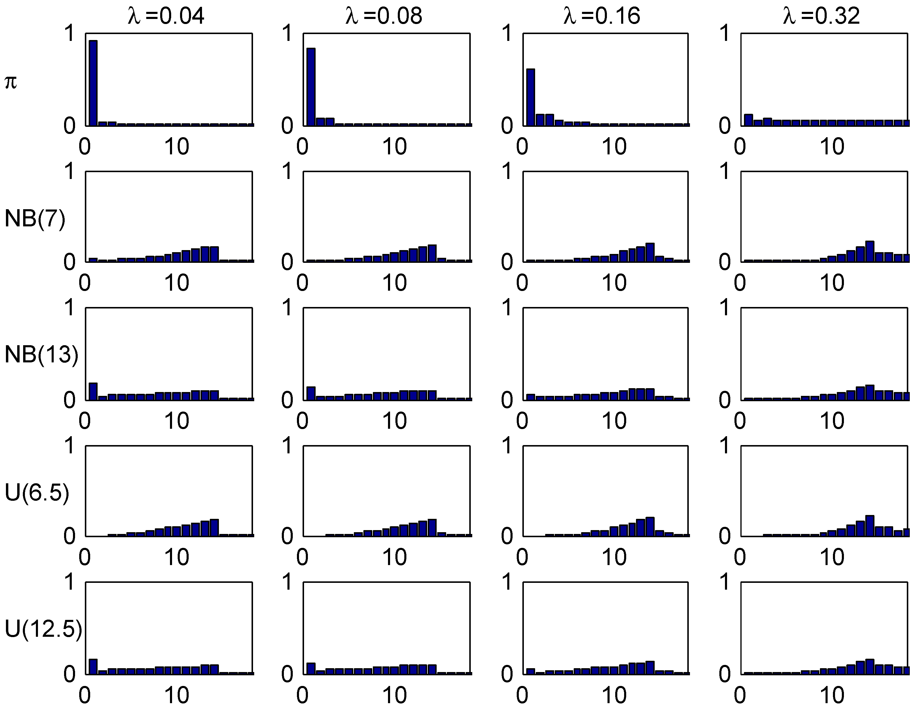
We selected four trial distributions for the distribution of the sojourn time A of a customer in the portfolio. Two are negative binomial with point probabilities
(i.e., A is distributed as where are independent geometric on ). Here ρ was chosen to make the means equal to 7 and 13, and the two distributions are denoted , resp. . The two other, denoted and , were taken as uniform distributions on , resp. , i.e., with roughly the same means. The distributions and their equilibrium distributions given by (5) are illustrated in Figure 1, giving the (yearly) probability mass function.
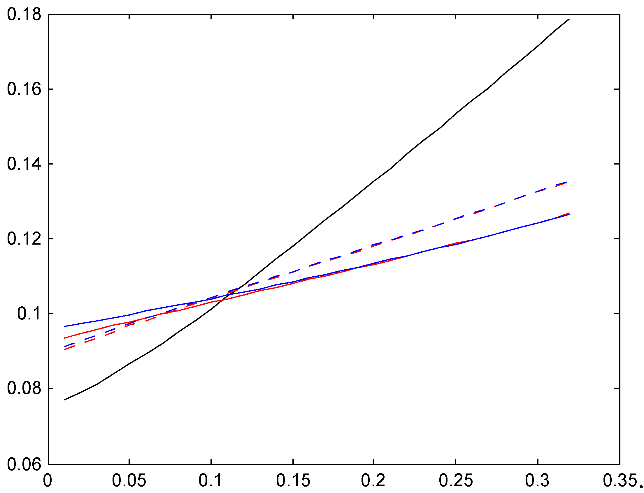
In the numerical calculations, the distributions were truncated at , except for Figure 2 where the truncation point was .
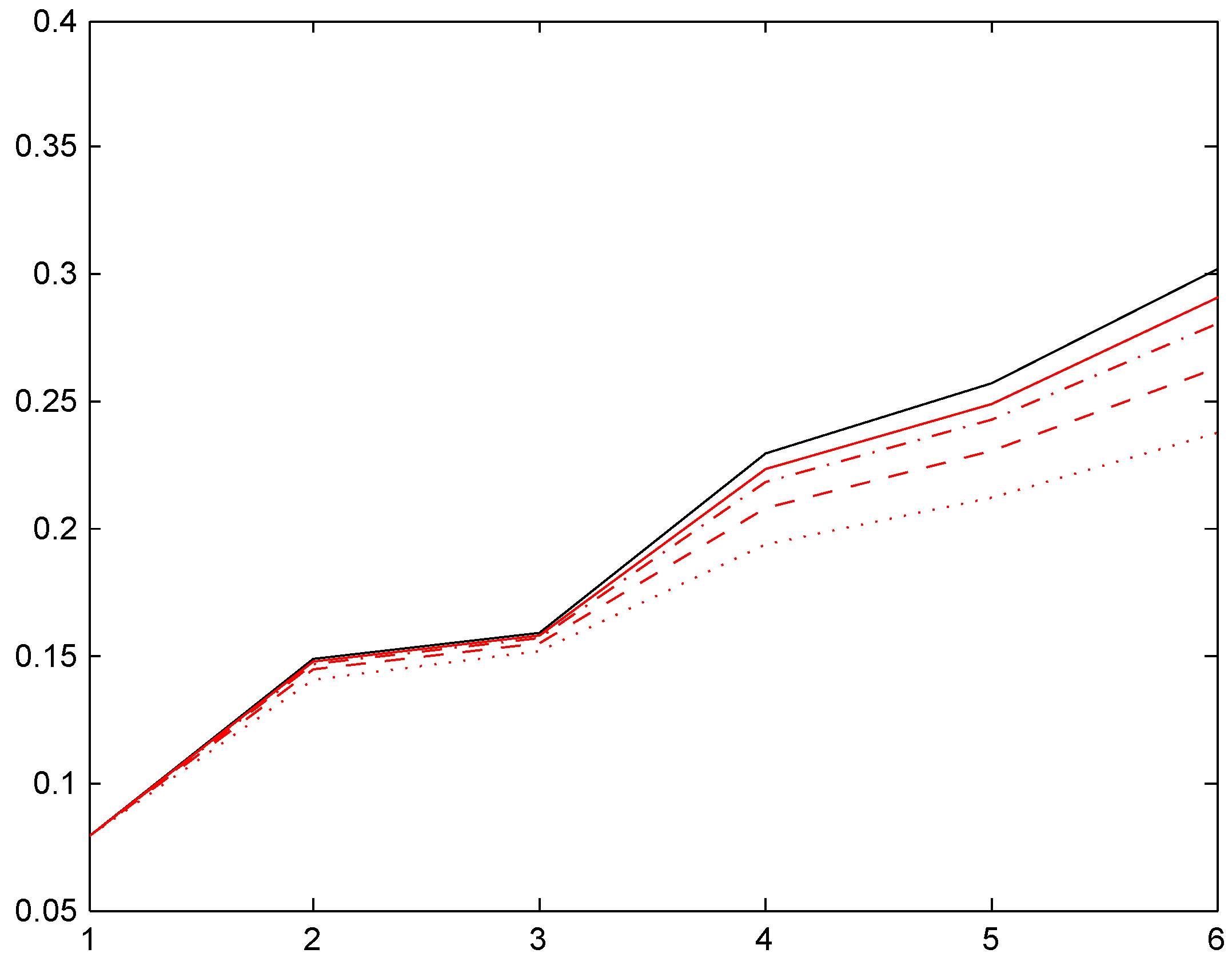
Figure 2.
Convergence of relativities, Ireland.

3.3. Bayesian Assumptions
We have taken the distribution U of the customers’ (yearly) λ parameter to be exponential with mean . The exponential assumption is from Bichsel [11], who fitted a gamma distribution to data and found the shape parameter to be close to 1. The value is from Lemaire & Zi ([12], p. 288) who argue this to be typical in many countries. 5
Motivated by this assumption, we have in many of the illustrations selected four values of λ, , , and , i.e., two below the population mean and two above. For the spread, note that and roughly correspond to the 5%, resp. 95%, quantiles in the exponential distribution with mean .
4. Convergence to Stationarity. Age-Corrected Distributions
4.1. Ireland
The Irish system is very simple with classes and transition rules as in Table 1. The initial class is .

| ℓ | ||||
|---|---|---|---|---|
| 6 | 100 | 5 | 6 | 6 |
| 5 | 90 | 4 | 6 | 6 |
| 4 | 80 | 3 | 6 | 6 |
| 3 | 70 | 2 | 5 | 6 |
| 2 | 60 | 1 | 4 | 6 |
| 1 | 50 | 1 | 3 | 6 |
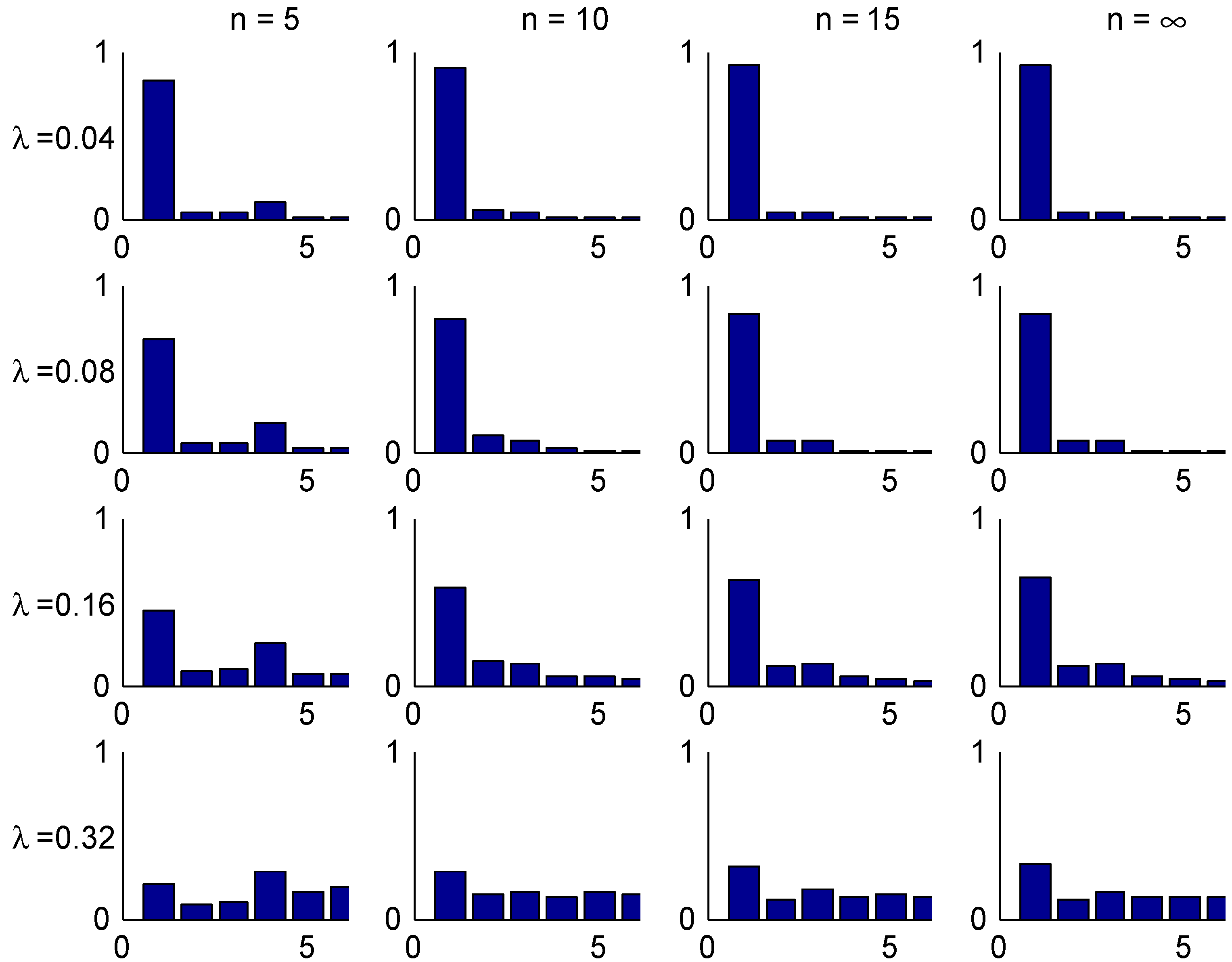
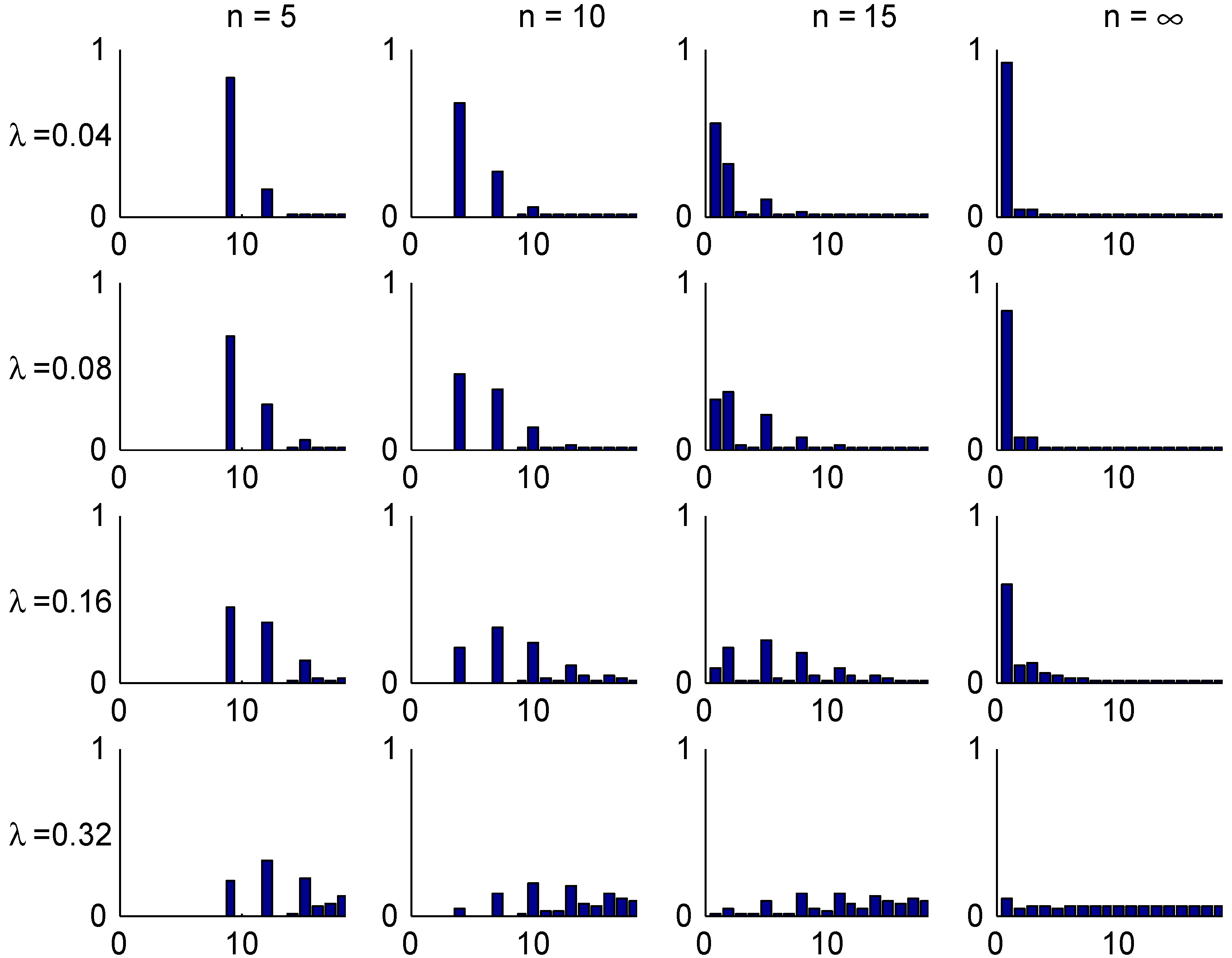
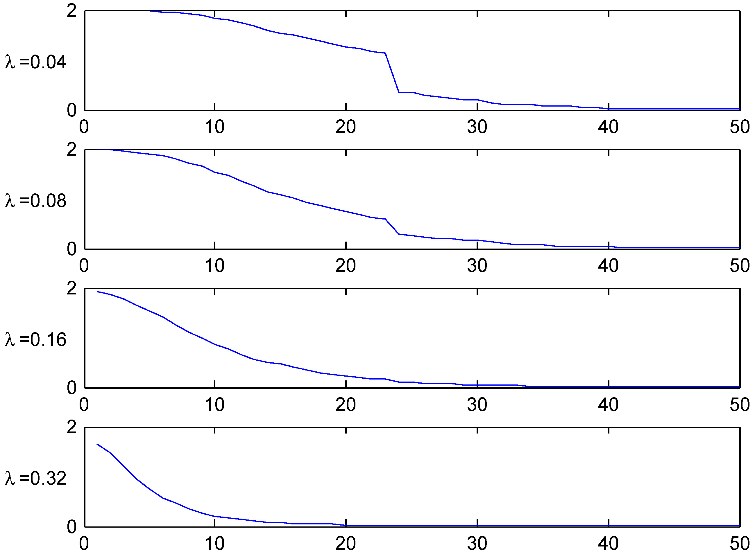
The convergence speed to the stationary distribution is illustrated in two figures. The first, Figure 3, shows the shape of the transient λ-distributions of for four selected values of n ( corresponds to the stationary distribution) and the four selected values of λ, and the next, Figure 4, plots the t.v. distance (2) to the stationary distribution as function of the number n of years elapsed.
Figure 3.
Transient distributions, Ireland.

The shape of these figures may be understood from the transition rules. Consider for example a customer with . Here most of the mass of π is concentrated in class 1, but class 1 can at earliest been reached in year 5. This explains the steep drop in Figure 4 in the t.v. distance between years 4 and 5. When looking at the bar plots in Figure 3 for the distribution of his class in different years, consider for example year 5 and note that w.p. he will have no claims in the first 5 years, so 0.82 is precisely the mass at class 1. W.p. he have will have exactly one claim. If this happens in year 0, his sequence of states in years 1,2,3,4,5 is . The similar sequences for a claim in year 1,2,3, resp. 4 are
Since any of the years 0,1,2,3,4 are equally likely for the claim. this explains that class 4 is more likely than classes 2,3, which is of course not the case for a good customer in stationarity (). The possibility of two or more claims giving mass in states 5,6 is just 0.02 and hence negligible.
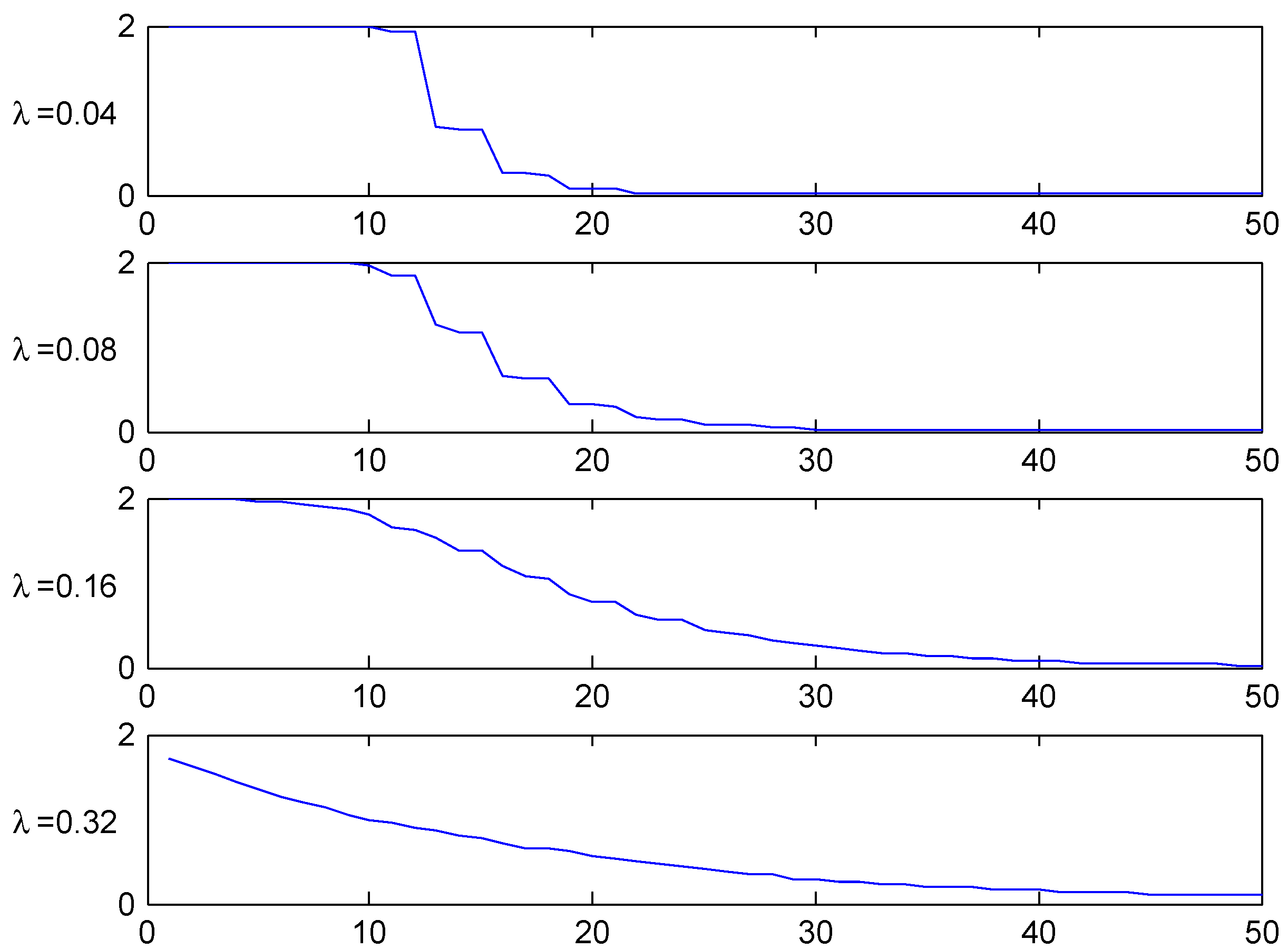
Figure 4.
T.v. convergence rate, Ireland.
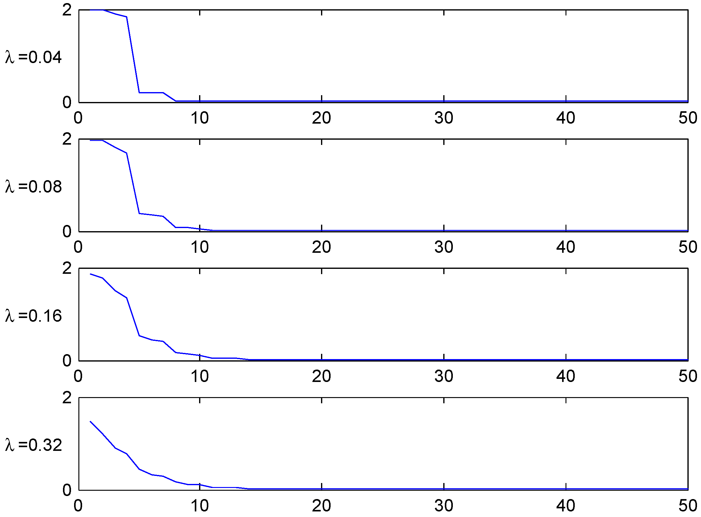
Similar remarks apply to other values of λ and n as well as the parallel figures for Italy and Germany to follow, but we shall not give the details.
The figures shows the fastest convergence rate among our three selected systems, and also that the rate is not that crucially depending on the value of λ. The explanation could be related to the simplicity of the Irish system.
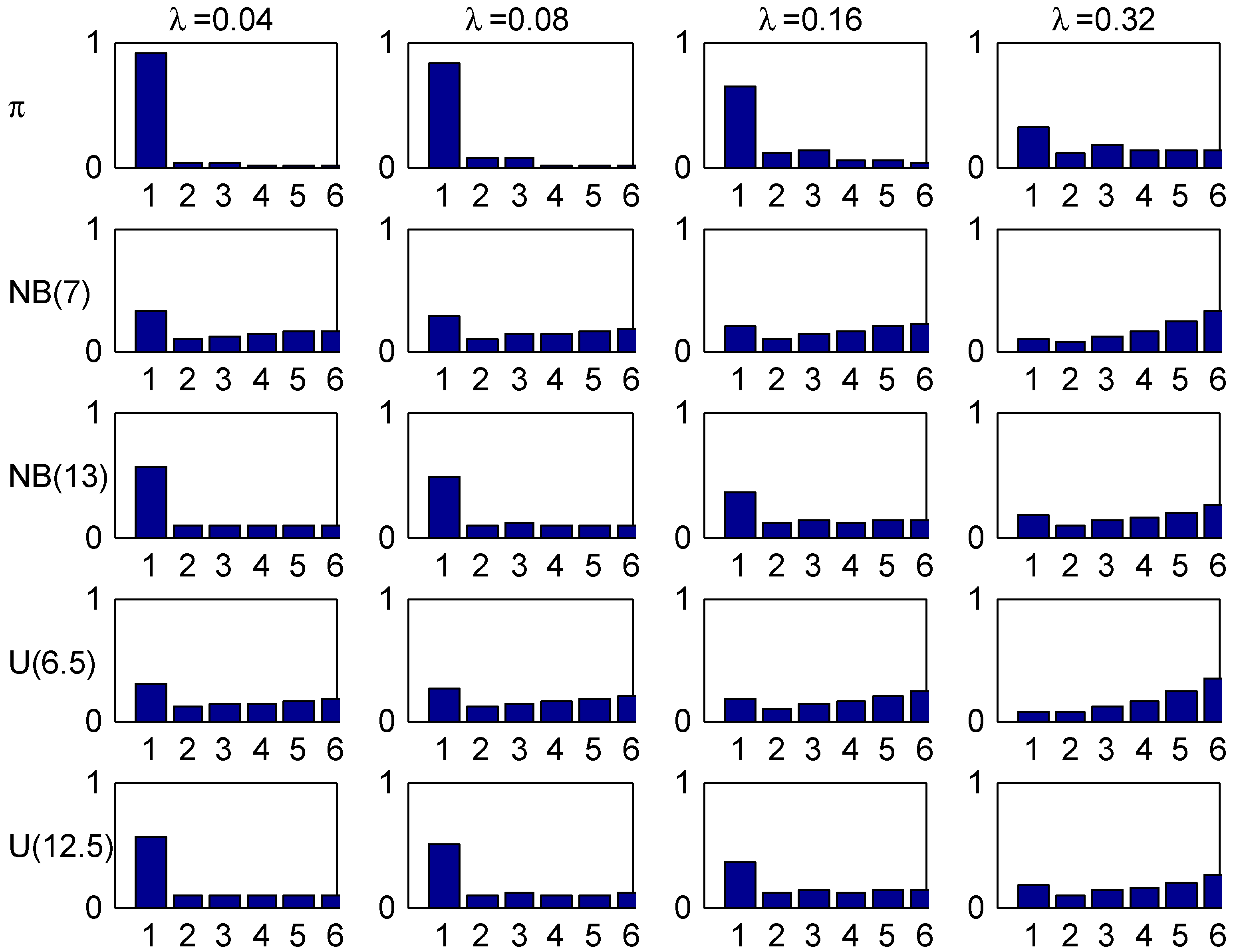
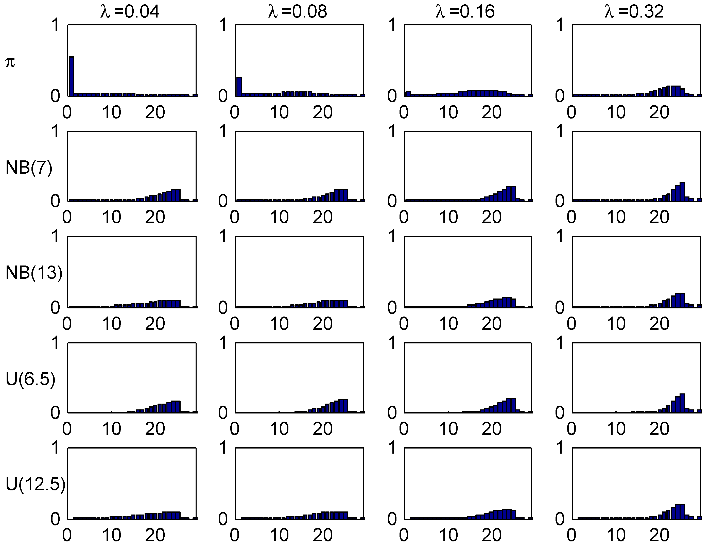
Figure 5, plots the age-corrected distribution for our four selected values of λ (one in each column) and our four trial distributions together with the stationary distribution (the benchmark of much literature) on top. It is seen that the agreement within columns is relatively good, with the most marked differences for small values of λ. The explanation could be the relatively fast convergence rate in the Irish system.
Figure 5.
Stationary and age-corrected distributions, Ireland.

4.2. Italy
The Italian system is intermediate with classes and transition rules as in Table 2. The initial class is [note that , a normalization allowed in exceptional cases].
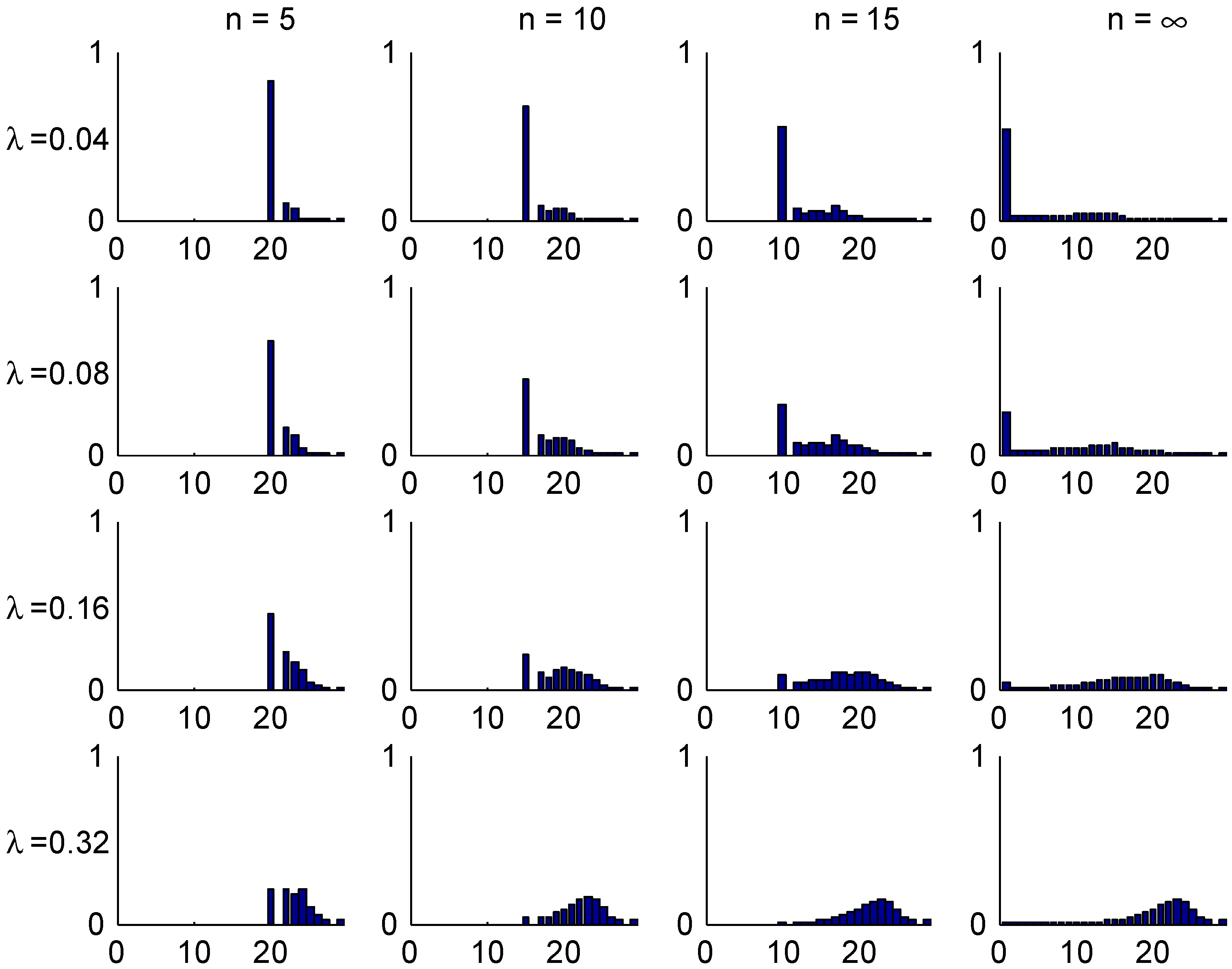
Figure 6 and Figure 7 are parallel to Figure 3 and Figure 4 for Ireland, illustrating the convergence speed to stationarity. As a new feature, we observe some gaps in the transient distributions. Consider for example where Figure 6 shows that classes 10 and 11 can not be attained. The explanation is that with 0 claims in years 0,1,2,3,4 one will go down 5 classes from 14 to 9, but with 1 claim one goes down 4 and up two, so to 12, and with more than two of course even higher. One sees also a somewhat slower rate of convergence to stationarity.
Finally the age-corrected distribution are plotted in Figure 8 together with the stationary distribution . One sees a marked worse agreement within columns than for Ireland. The most marked differences occur for small values of λ, with one feature being a considerable concentration of the (but not of ) close to the inital class 14. Again, the most natural explanation is the slow convergence rate.
| ℓ | ||||||
|---|---|---|---|---|---|---|
| 18 | 200 | 17 | 18 | 18 | 18 | 18 |
| 17 | 175 | 16 | 18 | 18 | 18 | 18 |
| 16 | 150 | 15 | 18 | 18 | 18 | 18 |
| 15 | 130 | 14 | 17 | 18 | 18 | 18 |
| 14 | 115 | 13 | 16 | 18 | 18 | 18 |
| 13 | 100 | 12 | 15 | 18 | 18 | 18 |
| 12 | 94 | 11 | 14 | 17 | 18 | 18 |
| 11 | 88 | 10 | 13 | 16 | 18 | 18 |
| 10 | 82 | 9 | 12 | 15 | 18 | 18 |
| 9 | 78 | 8 | 11 | 14 | 17 | 18 |
| 8 | 74 | 7 | 10 | 13 | 16 | 18 |
| 7 | 70 | 6 | 9 | 12 | 15 | 18 |
| 6 | 66 | 5 | 8 | 11 | 14 | 17 |
| 5 | 62 | 4 | 7 | 10 | 13 | 16 |
| 4 | 59 | 3 | 6 | 9 | 12 | 15 |
| 3 | 56 | 2 | 5 | 8 | 11 | 14 |
| 2 | 53 | 1 | 4 | 7 | 10 | 13 |
| 1 | 50 | 1 | 3 | 6 | 9 | 12 |
Figure 6.
Transient distributions, Italy.

Figure 7.
T.v. convergence rate, Italy.

Figure 8.
Stationary and age-corrected distributions, Italy.

4.3. Germany
The German system is rather elaborate. It has a large number of classes, , initial class 26, and quite detailed rules for the new class after one or more claims. For example, after one claim the customer moves up 14 classes when in class 1, always to class 17 when in classes 6–11, and up 3 classes when in classes 19–22. The rules for some selected cases are given in Table 3; for full details, see Meyer [9] or Mahmoudvand et al. [14].
| ℓ | ||||||
|---|---|---|---|---|---|---|
| 29 | 245 | 25 | 29 | 29 | 29 | 29 |
| 25 | 100 | 24 | 26 | 29 | 29 | 29 |
| 20 | 55 | 19 | 23 | 26 | 27 | 29 |
| 15 | 40 | 14 | 21 | 25 | 27 | 29 |
| 10 | 35 | 9 | 17 | 24 | 26 | 29 |
| 5 | 30 | 4 | 16 | 22 | 24 | 29 |
| 1 | 30 | 1 | 15 | 22 | 24 | 29 |
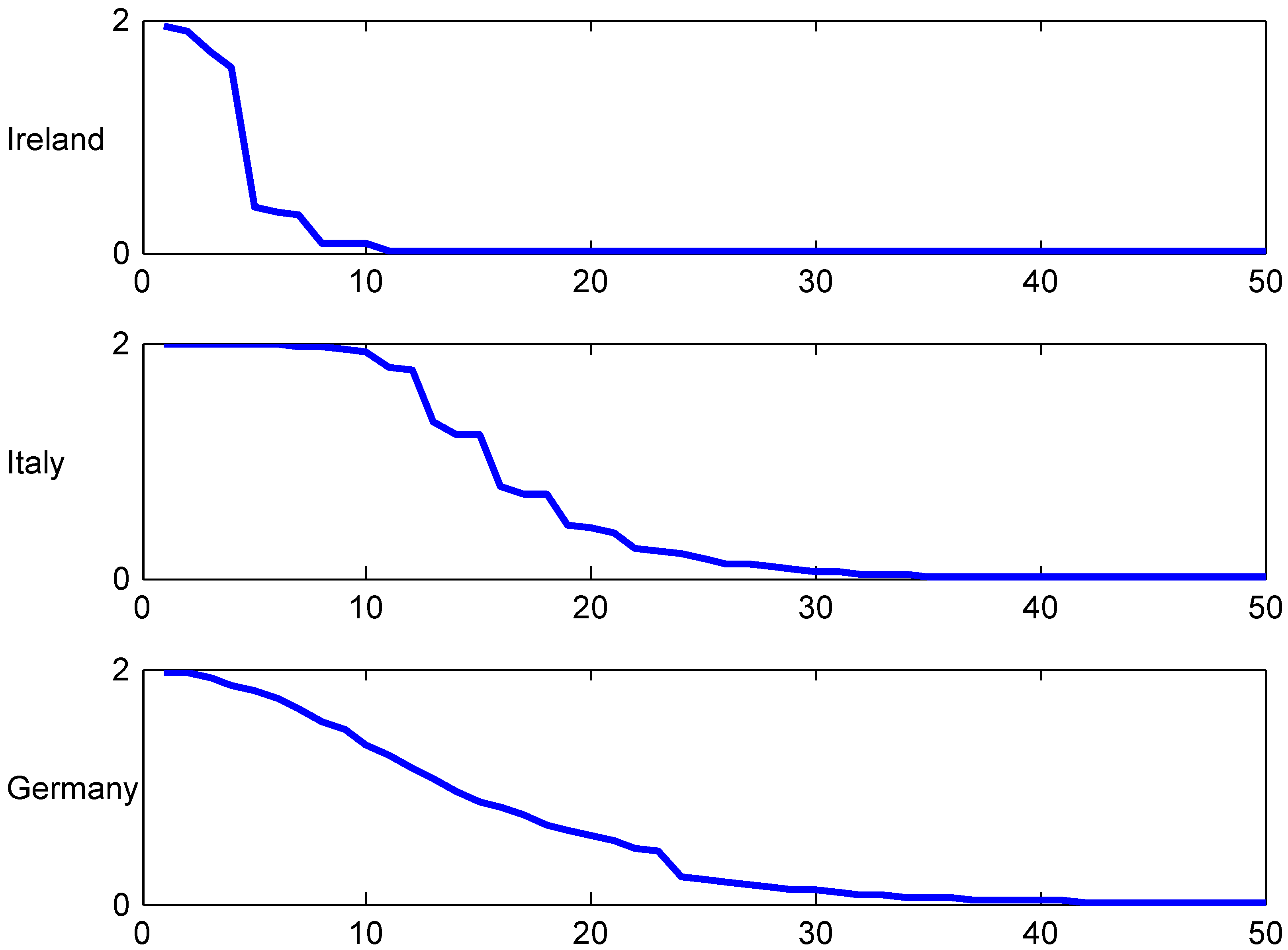
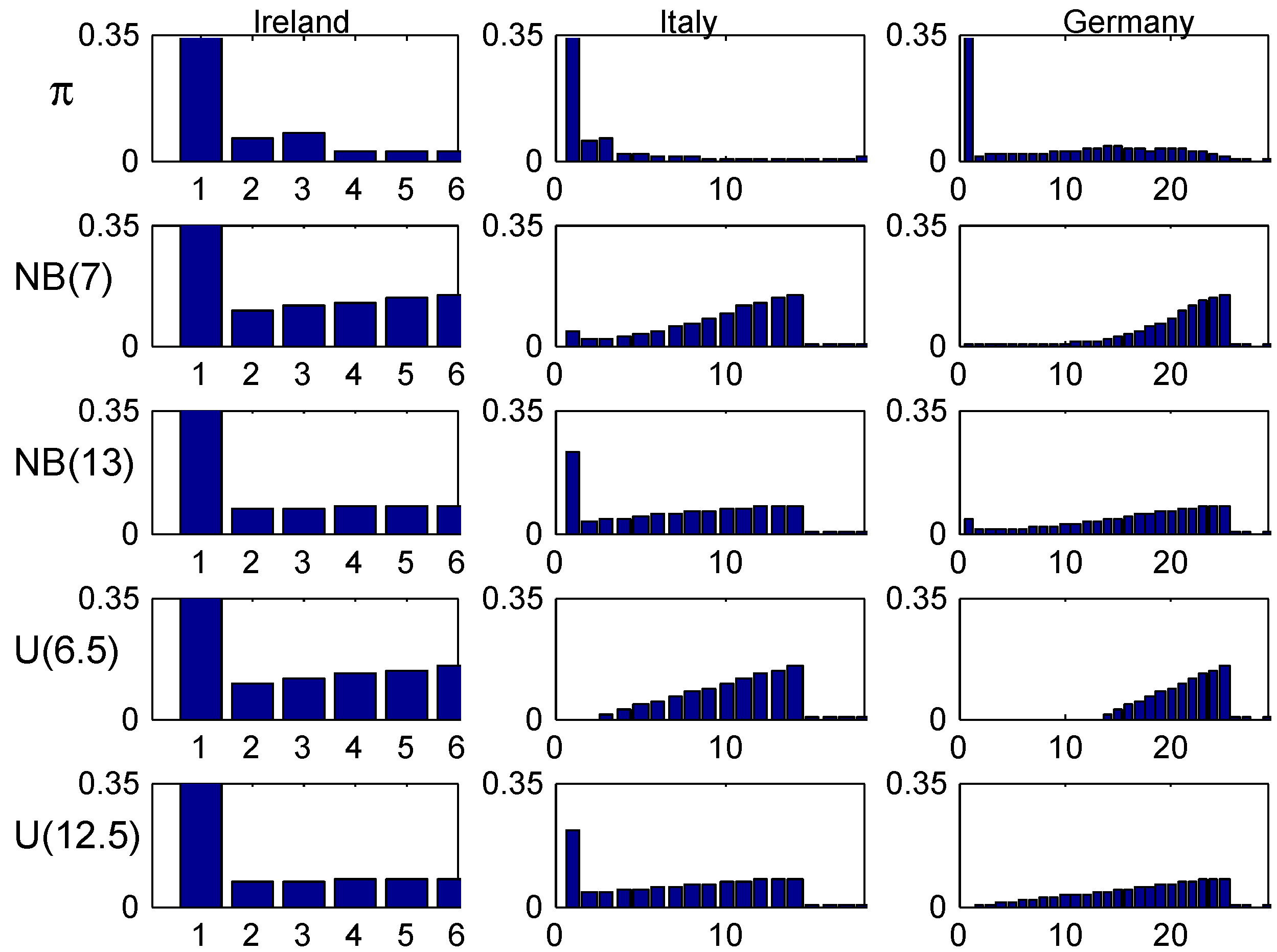
A quite special feature of the German system is the very high initial class, 26, meaning that a customer at earliest can reach the lowest premium level in class 1 after 25 years! This clearly shows up in the following Figure 9, Figure 10 and Figure 11, for example in the row in Figure 10 where the t.v. distance from the stationary distribution is substantial up to time , and in the comparisons of age-corrected distributions in Figure 11 which shows the same phenomenon as for Italy, a strong concentration of the (but not of ) close to the inital class 26.
Figure 9.
Transient distributions, Germany.

Figure 10.
T.v. convergence rate, Germany.

Figure 11.
Stationary and age-corrected distributions, Germany.

4.4. Population Averages
We believe the differentiation between high and low values of λ in the above figures is of interest rather than considering a single value as for example the population mean . However, the Bayesian view could motivate to summarize by averaging λ over the structure distribution U.
Figure 12.
Population averaged convergence rates: population mean 0.1.

Such averaging is done in Figure 12 and Figure 13. Figure 12 gives the population averaged t.v. distance
between the transient distribution at time n and the stationary distribution π, whereas Figure 13 gives the averaged age-corrected distributions .
These figures show essentially the same behavior as for the intermediate values 0.08 and 0.16 of λ, which could be expected since 0.04 and 0.32 are in the tails with low U-mass.
Figure 13.
Population averaged age-corrected distributions: population mean 0.1.

As a comparison, similar figures have been produced for the substantially smaller population mean 0.05, see Figure 14 and Figure 15. A first rough conclusion is that the behavior appears to be rather insensitive to the population mean.
Figure 14.
Population averaged convergence rates: population mean 0.05.

Figure 15.
Population averaged age-corrected distributions: population mean 0.05.
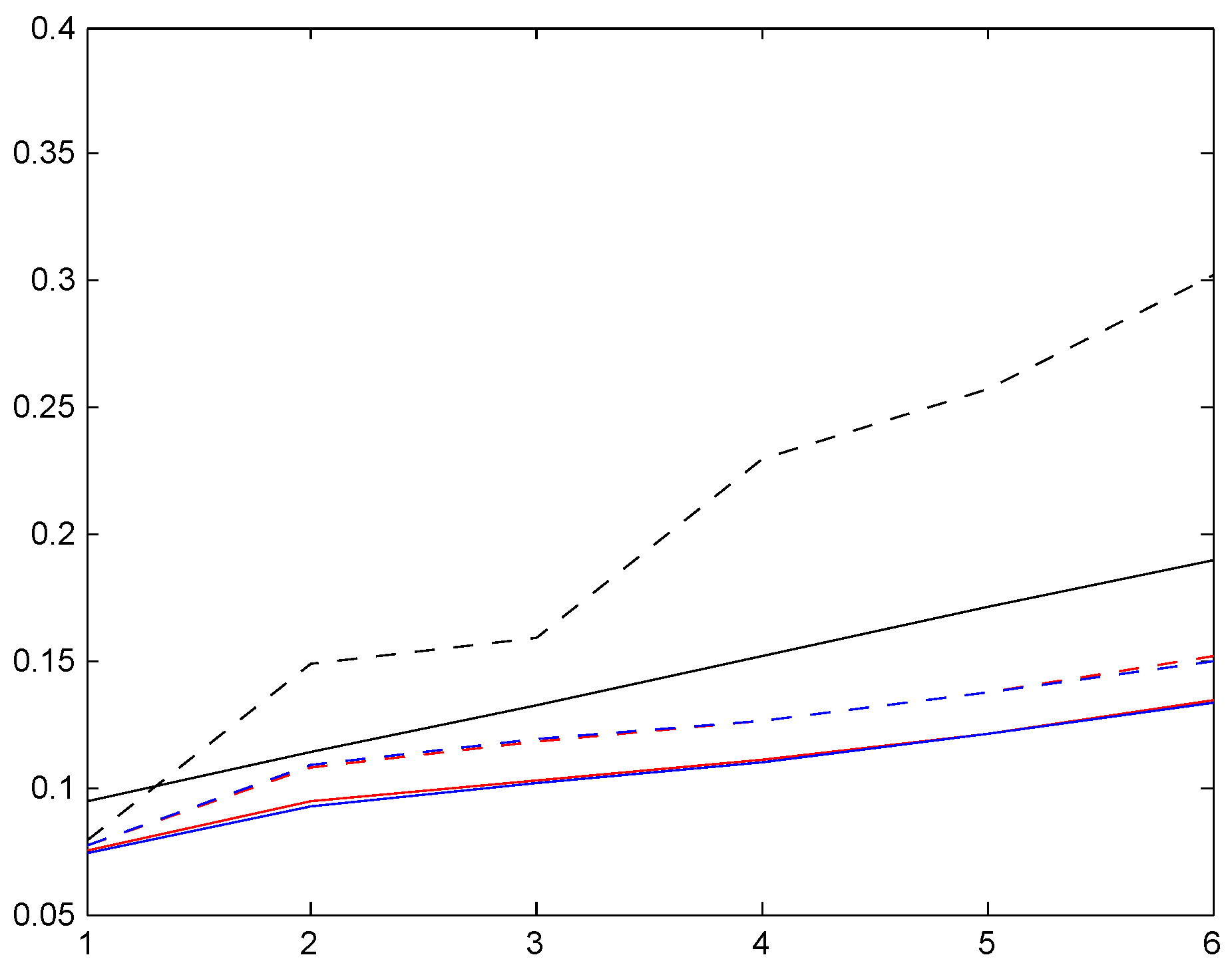
5. Relativities
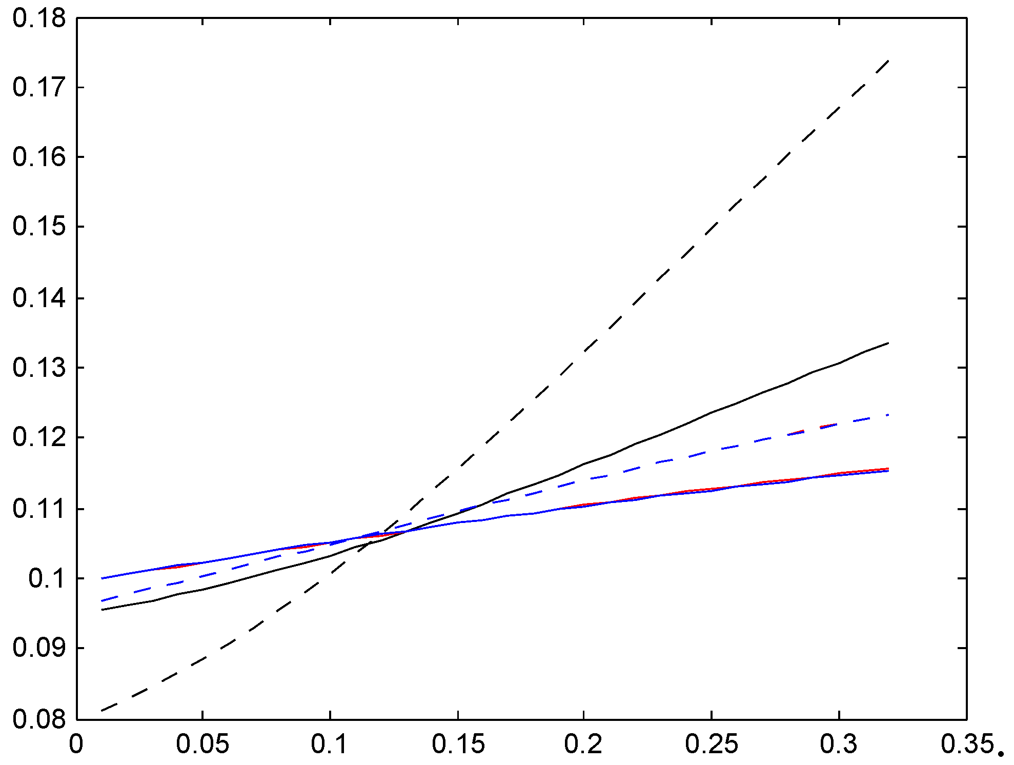
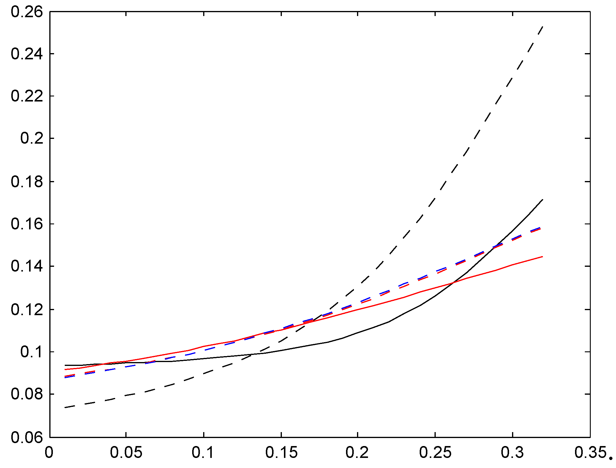
We now turn to the influence of finite customer sojourn times on the Bayes premium, proceeding as follows. For each of the three selected bonus systems and of the four trial sojourn time distributions, we first compute our age-corrected alternatives to the stationary distribution by means of (4) and next the Bayes premium in bonus class ℓ by means of the analogue of (3)
The results are in the following three Figure 16, Figure 17 and Figure 18. The legends are solid red for distribution , dotted red for , solid blue for , and dotted blue for . As supplement we also compute the Bayes premium corresponding to the stationary distribution (dotted black) and supplement with the premium corresponding to the given relativities for the bonus system (e.g., 50, 60, 70, 80, 90, 100 for Italy) in solid black; whereas the Bayes premium automatically yields financial equilibrium, cf. the discussion following (3), we here need to normalize to satisfy this requirement.
Figure 16.
Relativities, Ireland.

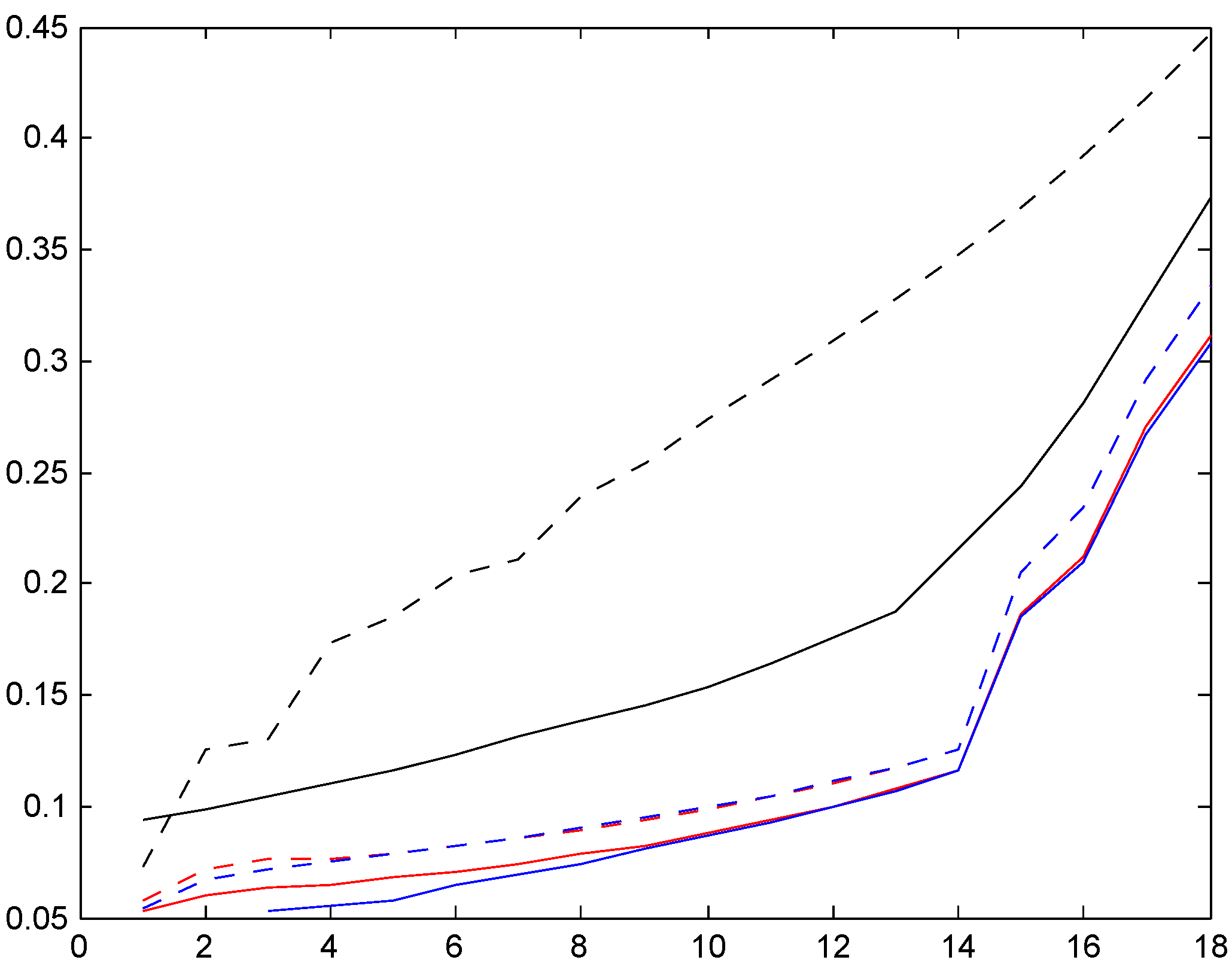
Figure 17.
Relativities, Italy.

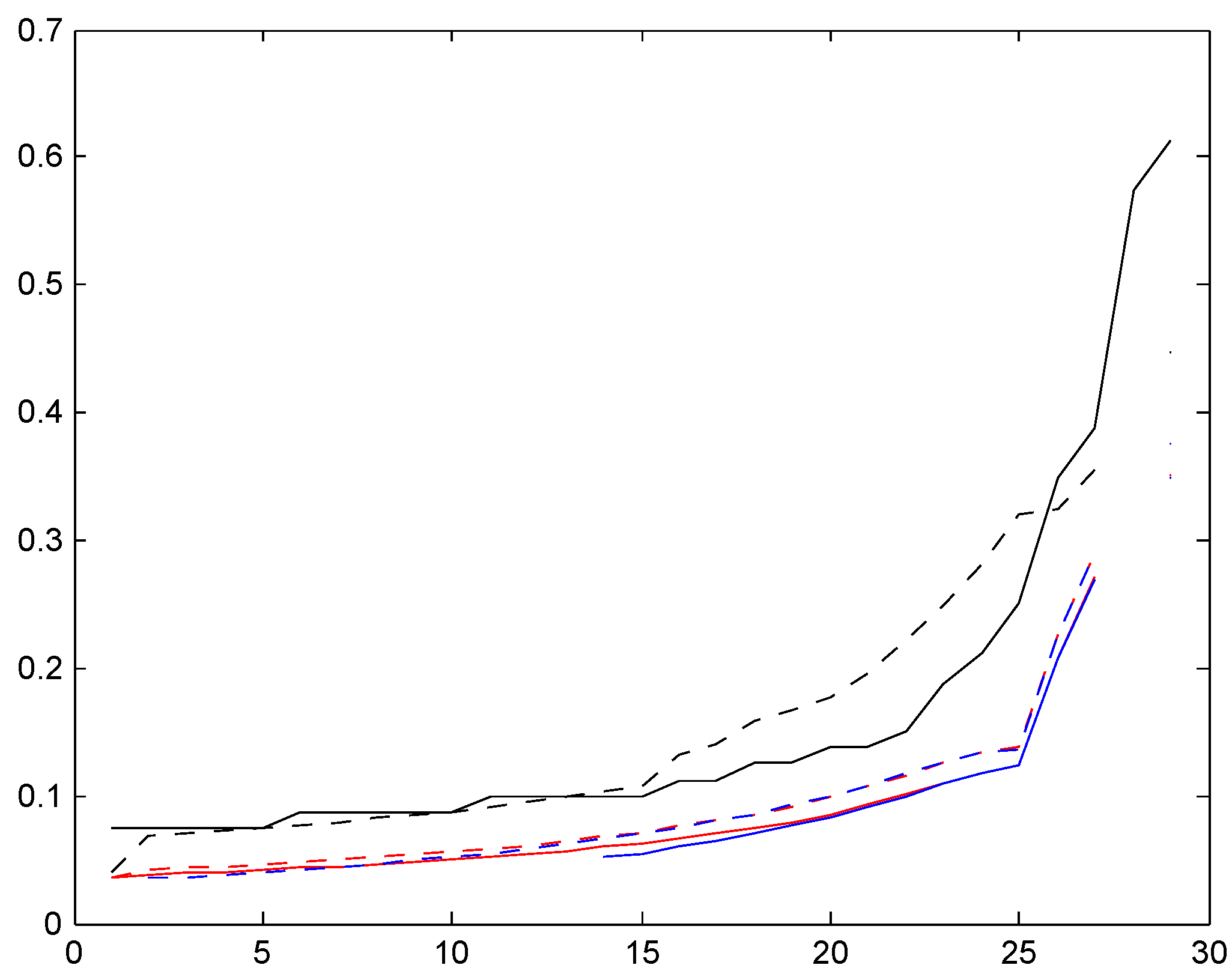
Figure 18.
Relativities, Germany.

When interpreting the figures, we first note that it does not contradict financial equilibrium that for a given country, one set of relativities is below the other. For example, all relativities corresponding to one of our four trial sojourn time distributions (colored graphs) are below the given relativities (solid black graph). But the explanation is simply that one set of relativities should be weighted with the age corrected distribution and the other with the stationary distribution, and the age corrected distributions have a region of importance which is more shifted towards high classes.
We next note that the two distributions , with the low mean are quite close, in some cases even hard to distinguish. Distributions , have a roughly doubled mean. As could be expected, this puts them closer to the Bayesian relativity computed w.r.t. . The convergence rate appears quite slow, however, and this is further illustrated in the following Figure 2. We took here the Irish system and compared the stationarity-based Bayesian relativity (solid black) to those of four versions of the negative binomial distribution (8), one with mean 10 (dotted red), one with mean 100 (dashed red), one with mean 200 (dash-dotted red), and one with mean 400 (solid red). The figure confirms the expectation of convergence, but shows also that (as just noted) it is slow.
6. Age-Corrected Average Premiums
Analogous with the stationarity-based definition (1) of the average premium of a λ-customer, we define the age-corrected version as
The are plotted in Figure 19, Figure 20 and Figure 21 one for each of the three bonus systems and the same 6 cases as for the relativities in Section 5, with the same legends.
We see a considerable difference between the two stationarity-based average premiums (solid black and dotted black) for Ireland and Italy, whereas they appear almost identical for Germany. The age-corrected average premiums are again quite different, and exhibit somewhat similar behavior as the relativities in Figure 16, Figure 17 and Figure 18.
Figure 19.
The , Ireland.

Figure 20.
The , Italy.

Figure 21.
The , Germany.
The ideal fairness criterion for a Bayesian premium rule is that the premium for a λ-customer should come as close to λ as possible. This can never be perfectly achieved: since the premium in the lowest bonus class is non-zero, a customer with a small λ will always pay too much, and since the premium in the highest class is finite, a customer with a large λ will always pay too little. The figures show that this effect is substantially more marked for the age-corrected average premiums than for the stationarity-based ones. The explanation is natural: if the customer has a finite sojourn time, the system will have less time to learn about his risk characteristics in the form of λ than if he had been there for ever, as is the (false) assumption underlying the stationarity-based calculations.
7. Concluding Remarks
In this paper, we have inspected how reasonable it is to view bonus-malus system via the stationary distribution, as is usually done. The conclusion is that in many cases the transient distributions are quite far from the stationary ones, and that this has considerable consequences on the computation of such quantities as Bayesian relativities and average premiums.
We do not necessarily insist that our trial distributions for the sojourn time in the portfolio have the relevant time span. A motor insurance may be terminated for example just if the insured gets a new car. In that case, he will typically continue with a new policy in the same company, but not enter in the same level as completely new insurers. Similar remarks to change of company, where usually some information on present bonus class or general previous claim statistics is passed from the old company to the new. Therefore, our choice of the A distributions should be seen as nothing more than scenario analysis.
Examples of numerical studies of special bonus-malus systems are, for example, in Lemaire [15], Lemaire & Zi [12] and Mahmoudvand et al. [14]. These papers differ from the present one by not going into the Bayesian aspect. Here the more closely related literature is Norberg [6] and Borgan et al. [3]. In particular, [3] contains ideas on how to get away from the stationary point of view. As analogue of our ,3] suggests a distribution of the form where the are suitable weights summing to one. It is also briefly mentioned that one interpretation corresponds to sampling a customer at random from the portfolio, but the connection to our which is obtained by taking is not given. Also the concept of sampling a customer at random is not explained very clearly, cf., e.g., our Theorem 1 and Appendix B below, and in key examples the are taken constant on an interval whereas is decreasing. Nevertheless, [3] contains some key ideas related to this paper, and to our mind, the paper has received surprisingly little attention in subsequent literature (but see Denuit et al. [1], Ch. 8).
Conflicts of Interest
The author declares no conflict of interest.
References
- M. Denuit, X. Marchal, S. Pitrebois, and J.F. Walhin. Actuarial Modelling of Claims Count. Chichester, UK: Wiley, 2007. [Google Scholar]
- J. Lemaire. Bonus-Malus Systems in Automobile Insurance. Boston, MA, USA: Kluwer, 1995. [Google Scholar]
- Ø. Borgan, J.M. Hoem, and R. Norberg. “A nonasymptotic criterion for the evaluation of automobile bonus systems.” Scand. Actuar. J. 1981 (1981): 165–178. [Google Scholar]
- H. Bühlmann. Mathematical Methods in Risk Theory. Berlin/Heidelberg, Germany: Springer-Verlag, 1970. [Google Scholar]
- H. Bühlmann, and A. Gisler. A Course in Credibility Theory and its Applications. Berlin/Heidelberg, Germany: Springer-Verlag, 2005. [Google Scholar]
- R. Norberg. “A credibility theory for automobile bonus system.” Scand. Actuar. J. 1976 (1976): 92–107. [Google Scholar] [CrossRef]
- N.E. Frangos, and S.D. Vontos. “Design of optimal bonus-malus systems with a frequency and a severity component on an individual basis in automobile insurance.” ASTIN Bull. 31 (2001): 1–22. [Google Scholar] [CrossRef]
- R. Mahmoudvand, and H. Hassani. “Generalized bonus-malus system with a frequency and a severity component on an individual basis in automobile insurance.” ASTIN Bull. 39 (2009): 307–315. [Google Scholar] [CrossRef]
- U. Meyer. Third Party Motor Insurance in Europe. Comparative Study of the Economical-Statistical Situation. Bamberg, Germany: University of Bamberg, 2000. [Google Scholar]
- S. Asmussen. Applied Probability and Queues, 2nd ed. New York, NY, USA: Springer-Verlag, 2003. [Google Scholar]
- F. Bichsel. “Erfahrungstariffierung in der Motorfahrzeug-Haftphlicht-Versicherung.” Mitt. Verein. Schweiz. Versich. Math., 1964, 119–130. [Google Scholar]
- J. Lemaire, and H. Zi. “A comparative analysis of 30 bonus-malus systems.” ASTIN Bull. 24 (1994): 287–309. [Google Scholar] [CrossRef]
- G.J. Tsougas. “Actuarial Modelling of Claims Counts and Losses in Motor Third Party Liability Insurance.” Ph.D. Thesis, University of Athens, Athens, Greece, 2013. [Google Scholar]
- R. Mahmoudvand, A. Edalati, and F. Shokooi. “Bonus-malus system in Iran: An empirical evaluation.” J. Data Sci. 11 (2013): 29–41. [Google Scholar]
- J. Lemaire. “A comparative analysis of most European and Japanese Bonus-malus systems.” J. Risk Insur. LV (1988): 660–681. [Google Scholar] [CrossRef]
- U. Grenander. “Some remarks on bonus systems in automobile insurance.” Scand. Actuar. J. 40 (1957): 180–197. [Google Scholar] [CrossRef]
- K. Loimaranta. “Some asymptotic properties of bonus systems.” ASTIN Bull. 6 (1972): 233–245. [Google Scholar]
- H. Bonsdorff. “On the convergence rate of bonus-malus systems.” ASTIN Bull. 22 (1992): 217–223. [Google Scholar] [CrossRef]
- T. Rolski, H. Schmidli, V. Schmidt, and J. Teugels. Stochastic Processes for Insurance and Finance. Chichester, UK: Wiley, 1999. [Google Scholar]
- S. Asmussen, and H. Albrecher. Ruin Probabilities, 2nd ed. Singapore, Singapore: World Scientific, 2010. [Google Scholar]
- J. Lemaire. Automobile Insurance: Actuarial Models. Boston, MA, USA: Kluwer, 1985. [Google Scholar]
Appendix
A. Proof of Theorem 2
For ease of notation, we suppress the dependency on λ. First note that satisfies
(multiply by on both sides). From this it follows easily by induction that
so
Rewriting (4) in matrix notation and using the independence of A and gives
B. A Variant of the Derivation of the Age-Corrected Distribution
A different way to arrive at distribution (4) as the relevant bonus class distribution in a model with finite sojourn times of customers is to ‘sieve customers one-by-one through the system’. By this we mean that we consider a sequence of λ-customers such that customer n has sojourn time and bonus classes during his time in the portfolio. We then define a -valued stochastic process Z as the sequence
and have:
Proposition 3. Assume that the distribution of A is non-lattice. Then the process Z given by (11) has limiting distribution given by (4).
This follows simply by noting that the instances where a new customer takes over in the construction of Z are regeneration points (the process starts afresh as from ) and appealing to the general theory of regenerative processes ([10], Ch. 6).
It should be noted, however, that Z is not a Markov chain. This follows by noting that
where is the time elapsed since the last regeneration point (backward recurrence time; for , for etc.). Here the distribution of depends on n, except for the special case where A is geometric, and so must (12) do (the argument excludes time-homogeneity, but also the Markov property can be seen to fail).
C. A More General Model
We here suggest a model which incorporates several features not covered by the basic bonus-malus model consider in the body of the paper.
We assume that a customer is characterized by a random mark M taking value in some set and a time-homogeneous Markov chain with state space where is the finite set of bonus classes and is finite or countable. We write ; is the number of claims in year , assumed Poisson with parameter , and is the bonus class. The initial class as well as depends on M.
In addition to potentially influencing the Poisson parameter, the Y component also generates the sojourn time A: it is assumed that the customer still in the portfolio in year will no longer be there in year w.p. , so that then . The further transition rules state that is calculated as a deterministic function of , and given , one has w.p. .
Example 2. To cover the classical model with independent sojourn time considered in the rest of the paper, take as the Poisson parameter of the customer and , . If A has some general distribution with point probabilities , , there are at least two ways to conform to the general framework above. Both are familiar from the theory of discrete phase-type distributions, ([10], III.4) or ([20], IX.1 and A5) (see in particular Sections IX.1 and A5 of [20]).
In the first, we take the state space for the Y-chain to be for some extra state Δ and . From state [corresponding to still being in the portfolio in year y] one can go only to either or Δ, w.p. for Δ and for (thus does not depend on ); state Δ (the coffin state) is absorbing. In the second, we take and w.p. . From , one goes always to , whereas state 0 is absorbing (thus if , if ). ☐
Example 3. Bonus hunger, i.e., the insured’s aptness not to file all small enough claims in order to avoid increase in future premiums, has been studied repeatedly in the literature. e.g., Lemaire [21] (see also Lemaire & Zi [12]) calculate for a given bonus system, each class ℓ and each λ a retention level , such that the insured’s costs in terms of either covering a claim of size Z himself or expected future premiums precisely balance when when he is in class ℓ. He will then file the claim if and not otherwise. The calculation is based on a distribution G of a claim Z. We can model this by simply modifying Example 2 by taking rather than . ☐
Example 4. An insured may be tempted to look for another insurer if he has had many recent claims, therefore a high bonus class and so (often without reason!) believes that his present insurer’s system is unfair. We can model this by modifying the first representation of A in Example 2 by allowing direct transitions from state n of y to the coffin state Δ, occuring with a probability depending on the present bonus class ℓ (typically will be increasing in ℓ). Thus
all other .
Example 5. Young or old drivers are generally considered to have risk characteristics different from the rest of the portfolio. We can model this by letting the mark M be the pair of the Poisson parameter Λ and (for a young driver) the year after the drivers license (or the age for an old driver), as well as a state of y to be of the form , with determining A as above and the updated year after the license. The initial class is then chosen as function of B, and one could have, e.g., that has the multiplicative form . ☐
Further examples, not spelled out in detail, are M including covariates entering multiplicatively in .
- 1These references have as their main theme not the Bayes premium but rather the credibility premium, also called the linear Bayes premium, computed as the minimizer of in the class of all linear functions of ; for the Gamma example and many others, the Bayes premium and the linear Bayes premium coincide. The motivation for considering linear predictors only is computational ease.
- 2Once this rule is chosen, one can also assert what is the optimal initial bonus level by a further mean square error minimization, cf. [6]. We do not go into this here.
- 3For convenience, the dependence on λ is suppressed in the notation. In the Bayesian set-up, a r.v. with a continuous distribution so that strictly speaking, a.s.; the set-up and statements then have to be understood in a suitable conditional sense.
- 4To be strict, one needs also to define some ordering of customers. These matters are to our mind of formal nature rather than intrinsically difficult, and so we omit the details.
- 5This value is also compatible with the data in a recent study of a Greek portfolio, Tsougas [13]. See, however, Section 4.4.
© 2014 by the author; licensee MDPI, Basel, Switzerland. This article is an open access article distributed under the terms and conditions of the Creative Commons Attribution license (http://creativecommons.org/licenses/by/3.0/).
Share and Cite
MDPI and ACS Style
Asmussen, S. Modeling and Performance of Bonus-Malus Systems: Stationarity versus Age-Correction. Risks 2014, 2, 49-73. https://doi.org/10.3390/risks2010049
AMA Style
Asmussen S. Modeling and Performance of Bonus-Malus Systems: Stationarity versus Age-Correction. Risks. 2014; 2(1):49-73. https://doi.org/10.3390/risks2010049
Chicago/Turabian StyleAsmussen, Søren. 2014. "Modeling and Performance of Bonus-Malus Systems: Stationarity versus Age-Correction" Risks 2, no. 1: 49-73. https://doi.org/10.3390/risks2010049