Neumann Series on the Recursive Moments of Copula-Dependent Aggregate Discounted Claims

Abstract

We study the recursive moments of aggregate discounted claims, where the dependence between the inter-claim time and the subsequent claim size is considered. Using the general expression for the $m-th$ order moment proposed by Léveillé and Garrido (Scand. Actuar. J. 2001, 2, 98–110), which takes the form of the Volterra integral equation (VIE), we used the method of successive approximation to derive the Neumann series of the recursive moments. We then compute the first two moments of aggregate discounted claims, i.e., its mean and variance, based on the Neumann series expression, where the dependence structure is captured by a Farlie–Gumbel–Morgenstern (FGM) copula, a Gaussian copula and a Gumbel copula with exponential marginal distributions. Insurance premium calculations with their figures are also illustrated.

1. Introduction

As the occurrence of catastrophe events becomes more frequent, the assumption of independence between event occurrence and claim severity is no longer sufficient in insurance risk modeling, given its impact on pricing and reserving, capital allocation solvency, as well as regulatory systems. The February 2009, Victorian bushfire in Australia (10,200 insurance claims amounting to approximately AUD 1.2 billion), the February 2011, Christchurch earthquake (USD 13 billion insured economic losses), the 2011 Great Eastern Japanese earthquake (loss amounting to as much as USD 40 billion), as well as the 2012 Hurricane Sandy (an expected loss of USD 25 billion) are the examples of this effect (see [1,2]).

In dealing with the dependency between the inter-claim arrivals and claim sizes, various approaches have been proposed in previous studies that can be noticed in [3,4,5,6,7,8,9,10,11], as well as the references therein. Regardless of the model used, we notice that previous research focused on either examining the expression of the moments of the aggregate discounted claims, $Z\left(t\right)$, as can be seen in [6,11,12,13,14], or by finding the related ruin measures and the ruin probability expressions, just like in [3,4,5,10,15].

Assuming the Poisson claim arrival process with claim sizes following mixed exponential distributions, [7] obtained the explicit expressions of the actuarial net premiums and the variances of the discounted aggregate claims from the Laplace transform of the distribution of the shot noise process, which was derived using the martingale approach. The first two moments of the aggregate discounted claims were obtained in [9] assuming the dependency between the claim sizes and the rates of claim occurrence affected by a Markovian environment, called the circumstance process. A delayed renewal process was also explored in [12,13,14,15], as well as [11] to accommodate the epochs between claim arrival and the observation of the risk process.

The asymptotical behaviour of a conditional tail probability dependence structure of claim sizes given the inter-claim arrival time was studied in [5,8]. Assuming that the conditional tail of claim size given the inter-claim time satisfies a certain condition for a bounded inter-claim time and a really huge claim size, [5] obtained the asymptotic tail probabilities of the discounted aggregate claims. Three copulas were indicated as fulfilling this assumption, which are the Farlie–Gumbel–Morgenstern (FGM) and the Frank and Ali–Mikhail–Haq (AMH) copulas, and the Weibull claim size was paired with exponential inter-claim arrival time in their numerical example. On the other hand, [8] explored the analytical properties related to the same dependence structure described by the survival copulas, such as their local and global uniformity.

Conditioning on the first arrival and using a renewal theory argument, [12] derived a useful expression for the $m-th$ recursive moment, whereby the inter-claim arrival time and the claim severity are assumed to be independent. The same conditioning argument was then applied in [6,10], assuming the FGM copula and then solved using the Laplace transform approach. More recently, [11] also adopted the same technique to derive the recursive moments of a Sparre Andersen risk process assuming a fairly general dependence structure between the inter-claim time and subsequent claim size variables, providing a simplified moments expression for assuming Erlang weights. Four types of copula were showcased in their examples of joint distribution between the said variables, which are the polynomial copula, the Bernstein copula, the generalized FGM copula, the extended FGM copula (references for these copulas are available in Section 3 of [11]).

The recursive moment equation resulting from the technique used in [6,12] takes the form of a Volterra integral equation of the second kind, which is widely used in the fields of mathematical physics, such as the electromagnetic and viscoelasticity fields, to represent the dynamics of materials that contain memory (refer to [16,17,18,19,20]). We are interested in using the same technique and then extend the recursive moments obtained in [6], so that it can be applied to any continuous bivariate distribution to accommodate the dependency between the two variables. To do so, we solve the recursive expression of the moments using the Neumann series obtained via the Picard method of successive approximations, upon which a selection of bivariate distributions can be applied, including bivariate copula.

This article is structured as follows. Section 2 will introduce the general framework of the continuous time renewal risk model together with its recursive moments with exponentially distributed inter-claim time and general claim size distribution. The dependency between the claim size and inter-claim time are then specified using a bivariate copula. For that purpose, we consider three copulas, which are the FGM copula, the Gaussian copula, which is a type of elliptical copula, and the Gumbel copula, an Archimedean type of copula, which is a natural candidate to represent an extreme value copula that caters for the one-sided dependence structure (see [21]).

In Section 3, we introduce the Volterra integral equation, which will be solved using the successive approximations method, leading to the Neumann series expression of the recursive moments, which is the main result of this paper. The Neumann series expression of the recursive moments allows the flexibility to capture various dependence structures provided by copula probability density functions (pdf).

Section 4 starts with the comparison between the value of moments obtained by our Neumann series expression assuming the FGM copula and the closed form solution by [6]. We then present the numerical analysis, showing the value of moments across the dependence parameter for each copula considered, assuming an exponentially distributed claim size. The illustration and comparison of moments, as well as premium values under the standard deviation principle are also included in this section. Section 5 concludes the article.

2. Model Setup

We consider a continuous time renewal risk model as in [6], whereby $\underline{Z}={\left\{Z\left(t\right)\right\}}_{t\ge 0}$ with:

$$Z\left(t\right)=\left\{\begin{array}{cc}\sum _{i=1}^{N\left(t\right)}{e}^{-\delta T_i}{X}_i\hfill & \text{if}N\left(t\right)>0\hfill \\ 0\hfill & \text{if}N\left(t\right)=0\hfill \end{array}\right.$$

In this model, $\underline{N}={\left\{N\left(t\right)\right\}}_{t\ge 0}$ is a homogeneous Poisson process and $X_i$ is a non-negative random variable (r.v.) representing the claim amount occurring at time $T_i$ for $i=1,2,\dots ,N\left(t\right)$. The instantaneous rate of net interest, δ, is assumed to be deterministic.

We also define the inter-claim time variable r.v. $W_j$ as:

$$W_j=\left\{\begin{array}{cc}{T}_j\hfill & \text{for}j=1\hfill \\ T_j-T_{j-1}\hfill & \text{for}j=2,3,\dots \hfill \end{array}\right.$$

The variables, $X_j$ and $W_j$, are assumed to be continuous. In this study, we relax the independent assumption between the inter-claim time, $W_j$, and the claim size, $X_j$, and we let $\left\{\right(X_j$,$W_j{\left)\right\}}_{j\in \mathbb{N}}$ to form a sequence of independent and identically distributed (i.i.d) random vectors, whose components are dependent.

2.1. Recursive Moments of Aggregate Discounted Claims

Conditioning on the arrival of the first claim as in [6,10,12], and knowing that $\mathbf{E}\left(X^m\right|W=s)={\int }_0^{\infty }{x}^m{f}_{X|W=s}\left(x\right)dx$ for $m\ge 1$, we have the general form of the $m-th$ moments of aggregate discounted claim as the following:

$$\begin{array}{cc}\hfill {\mu }_Z^{\left(m\right)}\left(T\right)=\mathbf{E}\left[Z^m\left(T\right)\right]& ={\int }_0^T{f}_W\left(s\right)e^{-m\delta s}\mathbf{E}\left(X^m\right|W=s)ds+{\int }_0^T{f}_W\left(s\right)e^{-m\delta s}{\mu }_Z^{\left(m\right)}(T-s)ds\hfill \\ & +\sum _{j=1}^{m-1}\left(\genfrac{}{}{0pt}{}{m}{j}\right){\int }_0^T{f}_W\left(s\right)e^{-m\delta s}\mathbf{E}\left(X^j\right|W=s){\mu }_Z^{(m-j)}(T-s)ds\hfill \\ & ={\int }_0^T{\int }_0^{\infty }{e}^{-m\delta s}{x}^m{f}_{X,W}\left(x,s\right)dxds+{\int }_0^T{e}^{-m\delta s}{f}_W\left(s\right){\mu }_Z^{\left(m\right)}(T-s)ds\hfill \\ & +\sum _{1\le j<m}\left(\genfrac{}{}{0pt}{}{m}{j}\right){\int }_0^T{\int }_0^{\infty }{e}^{-m\delta s}{x}^j{f}_{X,W}\left(x,s\right){\mu }_Z^{(m-j)}(T-s)dxds\hfill \end{array}$$

(1)

where $f_{X,W}\left(x,s\right)$ is the bivariate probability density function (pdf) of the pair, $X_j$ and $W_j$.

In this study, the joint pdf is described via a copula, $C_{\theta }(u,v)$, whose pdf is given by $c_{\theta }(u,v)=\frac{d^2}{dudv}{C}_{\theta }(u,v)$ with dependence parameter θ (see, e.g., [22,23] for a general review on copulas). The bivariate pdf of $(X,W)$ at $(x,s)$ can be represented as:

$$f_{X,W}(x,s)=c_{\theta }(F_X\left(x\right),F_W\left(s\right))f_X\left(x\right)f_W\left(s\right)$$

where $f(·)$ and $F(·)$ are the marginal pdf and cdf for r.v.’s X and W.

Since the jump occurrences are assumed to follow a Poisson distribution, we therefore have an exponentially distributed inter-claim arrival time, i.e., $W\sim exp\left(\beta \right)$. Upon replacing $f_W\left(s\right)=\beta e^{-\beta s}$, we obtain:

$$\begin{array}{cc}\hfill {\mu }_Z\left(T\right)& ={\int }_0^T{\int }_0^{\infty }\beta x{e}^{-(\beta +\delta )s}{f}_X\left(x\right)c_{\theta }\left(F_X\left(x\right),F_W\left(s\right)\right)dxds+\beta {\int }_0^T{e}^{-(\beta +\delta )s}{\mu }_Z(T-s)ds\hfill \\ & =C\left(T\right)+\beta {\int }_0^T{e}^{-(\beta +\delta )s}{\mu }_Z(T-s)ds\hfill \\ & =C\left(T\right)+\beta {\int }_0^T{e}^{-(\beta +\delta )(T-s)}{\mu }_Z\left(s\right)ds\hfill \end{array}$$

(2)

and:

$$\begin{array}{cc}\hfill {\mu }_Z^{\left(m\right)}\left(T\right)& =\beta [{\int }_0^T{\int }_0^{\infty }{x}^m{e}^{-(\beta +m\delta )s}{f}_X\left(x\right)c_{\theta }\left(F_X\left(x\right),F_W\left(s\right)\right)dxds\hfill \\ & +\sum _{1\le j<m}\left(\genfrac{}{}{0pt}{}{m}{j}\right){\int }_0^T{x}^{-(m-j)}{e}^{-[\beta +m\delta ]s}{c}_{\theta }\left(F_X\left(x\right),F_W\left(s\right)\right)f_X\left(x\right){\mu }_Z^{(m-j)}(T-s)dxds]\hfill \\ & +\beta {\int }_0^T{e}^{-(\beta +m\delta )s}{\mu }_Z^{\left(m\right)}(T-s)ds\hfill \\ & =C^{\left(m\right)}\left(T\right)+\beta {\int }_0^T{e}^{-(\beta +m\delta )s}{\mu }_Z^{\left(m\right)}(T-s)ds\hfill \\ & =C^{\left(m\right)}\left(T\right)+\beta {\int }_0^T{e}^{-(\beta +m\delta )(T-s)}{\mu }_Z^{\left(m\right)}\left(s\right)ds\hfill \end{array}$$

(3)

where

$$\begin{array}{cc}\hfill C^{\left(m\right)}\left(T\right)& =\beta [{\int }_0^T{\int }_0^{\infty }{x}^m{e}^{-(\beta +m\delta )s}{f}_X\left(x\right)c_{\theta }\left(F_X\left(x\right),F_W\left(s\right)\right)dxds\hfill \\ & +\sum _{1\le j<m}\left(\genfrac{}{}{0pt}{}{m}{j}\right){\int }_0^T{x}^{-(m-j)}{e}^{-[\beta +m\delta ]s}{c}_{\theta }\left(F_X\left(x\right),F_W\left(s\right)\right)f_X\left(x\right){\mu }_Z^{(m-j)}(T-s)dxds]\hfill \end{array}$$

(4)

for $m=2,3,\cdots$.

2.2. Copula Used

We are interested to calculate the first, second and mth moment of aggregate discounted claims under three copulas: the FGM copula, the Gaussian copula and the Gumbel copula. Their pdfs are given by:

$$c_{\theta }^F\left(F_X\left(x\right),F_W\left(s\right)\right)=1+\theta (1-2F_X\left(x\right))(1-2F_W\left(s\right))$$

(5)

$$c_{\theta }^G\left(F_X\left(x\right),F_W\left(s\right)\right)=\frac{1}{\sqrt{\left(1-{\theta }^2\right)}}{e}^{-\frac{\theta (2{\Phi }^{-1}\left(F_X\left(x\right)\right){\Phi }^{-1}\left(F_W\left(s\right)\right)-\theta ({\Phi }^{-1}{\left(F_X\left(x\right)\right)}^2+{\Phi }^{-1}{\left(F_W\left(s\right)\right)}^2))}{2({\theta }^2-1)}}$$

(6)

$$\begin{array}{cc}\hfill c_{\theta }^M(F_X\left(x\right),F_W\left(s\right))& =\frac{{(-lnu)}^{\theta }}{-ulnu}\frac{{(-lnv)}^{\theta }}{-vlnv}\frac{\sqrt[\theta ]{{(-lnu)}^{\theta }+{(-lnv)}^{\theta }}}{{[{(-lnu)}^{\theta }+{(-lnv)}^{\theta }]}^2}\hfill \\ & \times \frac{\sqrt[\theta ]{{(-lnu)}^{\theta }+{(-lnv)}^{\theta }}+\theta -1}{e^{\sqrt[\theta ]{{(-lnu)}^{\theta }+{(-lnv)}^{\theta }}}}\hfill \end{array}$$

(7)

The FGM copula is used in this study due to its simplicity and analytical tractability. It is also used to verify our numerical results in Section 4.1 with [6]. The well-known elliptical family member, the Gaussian copula, is chosen as, to the best of our knowledge, the effect of elliptical copula in terms of the dependence between claim size and inter-claim time have not been explored extensively. The Gumbel copula is also chosen, since it could be adopted by an insurance company, who assumes risks with extreme magnitude, having the tendency to occur together, as pointed out by De Matteis in [21]. Many standard statistical texts offer illustrations of copula scatter plots with various dependence structure, for which we refer to [22,23,24].

3. Linear Integral Equations

The most general form of linear integral equation (IE) is given by:

$$\begin{array}{c}\hfill h\left(T\right)\Psi \left(T\right)=g\left(T\right)+{\int }_a^{b\left(T\right)}K(T,s)\Psi \left(s\right)ds\end{array}$$

(8)

where $\Psi \left(T\right)$ is the solution to the IE that we need to obtain, $g\left(T\right)$ is a given function and $K(T,s)$ is the kernel for the IE. Equation (8) can be a homogeneous/non-homogenous, Volterra/Fredholm IE of the 1st/the 2nd kind, for which readers are referred to the conditions given in Section 2.1 of [18]. Linear IE can be solved either numerically using methods, such as the Runge–Kutta and collocation methods (see, e.g., [25,26]), or solved explicitly, such as by obtaining its Neumann series via the Picard method of successive approximations or using the Laplace transform method.

3.1. Volterra IE of the 2nd Kind

If we have $g\left(T\right)\ne 0$, $h\left(T\right)=1$, and $b\left(T\right)=T$, Equation (8) becomes:

$$\begin{array}{c}\hfill \Psi \left(T\right)=g\left(T\right)+{\int }_a^{T}K(T,s)\Psi \left(s\right)ds\end{array}$$

(9)

which is a non-homogeneous Volterra integral equation of the second kind. The Volterra IE is widely used in the areas of viscoelasticity and electromagnetic to compute the dynamics of materials that “contain” memory, other than being useful in renewal theory and demography (see, e.g., [16,27], as well as the references therein for a more rigorous treatment on Volterra integral equations).

We easily notice that the moments provided by Equation (2) and Equation (3) take the form of Equation (9) and attempt to derive the explicit solution of the recursive expressions using Neumann series in the next subsection.

A unique and continuous solution, $\Psi \left(T\right)$, is obtainable if we have a combination of a continuous kernel, $K(T,s)$, in the region $a\le s\le T\le b\left(T\right)$ with a function, $g\left(T\right)$, that is continuous in the region $a\le T\le b\left(T\right)$, even though it is not a requirement for the kernel function, $K(T,s)$, to be continuous (see page 1 of [28] and page 5 of [20]). For the case of a discontinuous kernel function, we need to check if $K(T,s)$ fulfills the three regularity conditions set on page 3 of [27], and, hence is an $L^2$-function.

In the case of the first and second moments, ${\mu }_Z\left(T\right)$ and ${\mu }_Z^{\left(2\right)}\left(T\right)$, the function, $g\left(T\right)$, is represented by the following equations, respectively:

$$\begin{array}{c}\hfill {\int }_0^T{\int }_0^{\infty }{e}^{-(\beta +\delta )s}x{f}_X\left(x\right)c_{\theta }\left(F_X\left(x\right),F_W\left(s\right)\right)dxds\end{array}$$

(10)

$$\begin{array}{c}\hfill {\int }_0^T{\int }_0^{\infty }{e}^{-(\beta +2\delta )s}{x}^2{f}_X\left(x\right)c_{\theta }\left(F_X\left(x\right),F_W\left(s\right)\right)dxds\end{array}$$

$$\begin{array}{c}\hfill +2{\int }_0^T{\int }_0^{\infty }{e}^{-(\beta +2\delta )s}x{f}_X\left(x\right)c_{\theta }\left(F_X\left(x\right),F_W\left(s\right)\right){\mu }_Z(T-s)dxds\end{array}$$

(11)

where $F_W\left(s\right)=1-e^{-\beta s}$ is the inter-claim time cdf.

As X and W are continuous r.v.’s, and by corollary 2.2.6 of [23] on copula continuity, $g\left(T\right)$ is the continuous function for $s\in [0,T]$ and $x\in [0,\infty ]$, since it is the sum and product of continuous functions. The kernel function is also continuous, as it is an exponential function given by:

$$K(T,s)=e^{-(\beta +m\delta )(T-s)}$$

(12)

Additionally, it is a bounded function in the square $\Pi =\left\{\right(T,s):a\le T\le b(T),a\le s\le T\}$.

3.2. Neumann Series

In this section, we will find the Neumann series of the Volterra IE assuming the exponentially distributed inter-claim arrival time and a general claim size with continuous pdf. To do so, we start with a proposition from Chapter 3 of [27], which used the Picard method of successive approximation.

Proposition 1. Neumann Series for a Volterra IE of the 2nd Kind

For the Volterra IE of the 2nd kind, as in Equation (9), where $g\left(T\right)$ and $K(T,s)$ are $L^2$-functions, its Neumann series is given by:

$$\begin{array}{cc}\hfill \Psi \left(T\right)& =g\left(T\right)+\sum _{n=1}^{\infty }{\lambda }^n{\int }_a^{T}K(T,s)\Psi \left(s\right)ds\hfill \\ & =g\left(T\right)+\lambda {\int }_a^T\sum _{n=1}^{\infty }{\lambda }^{n-1}{K}_n(T,s)g\left(s\right)ds\hfill \\ & =g\left(T\right)+\lambda {\int }_a^T\Gamma (T,s;\lambda )g\left(s\right)ds\hfill \end{array}$$

(13)

where $\Gamma (T,s;\lambda )={\sum }_{n=1}^{\infty }{\lambda }^{n-1}{K}_n(T,s)$ is the unique resolvent kernel and $K_n(T,s)$ is the n-th-iterated kernel function satisfying the recurrence formula:

$$\begin{array}{c}\hfill K_n(T,s)={\int }_s^{T}K(T,u)K_{n-1}(u,s)du\end{array}$$

(14)

with $K_1(T,s)=K(T,s)$.

In order to prove our theorem, it is necessary to find the resolvent kernel, which is obtained in the following lemma.

Lemma 2. Consider the kernel function given by Equation (12). For $m=1,2,\dots$, its resolvent kernel is therefore given by:

$$\begin{array}{c}\hfill \Gamma (T,s;\lambda )=e^{-m\delta (T-s)}\end{array}$$

(15)

Proof. Using Equation (14), we obtain K${}_2(T,s),K_3(T,s),\cdots ,K_{n+1}(T,s)$ starting from $K(T,s)=K_1(T,s)=e^{-(\beta +m\delta )(T-s)}$. Letting $(T-s)=-(s-T)$ and since ${(s-T)}^n={[-(s-T)]}^n$ for even n, the resolvent kernel is then obtained by summing up $K_m(T,s)$ as follows:

$$\begin{array}{cc}\hfill \Gamma (T,s;\lambda )& =e^{-(m\delta +\beta )(T-s)}\sum _{n=1}^{\infty }\frac{{[-(s-T)\beta ]}^n}{n!}\hfill \\ & =e^{-(m\delta +\beta )(T-s)}{e}^{-\beta (T-s)}\hfill \\ & =e^{-m\delta (T-s)}\hfill \end{array}$$

☐

Now, we can obtain the expression for the first and second moment, which is the main result of this article.

Theorem 3. The explicit solution of the first two moments are given by:

$$\begin{array}{cc}\hfill {\mu }_Z\left(T\right)& ={\int }_0^T{\int }_0^{\infty }{e}^{-\delta s}x{\mathfrak{L}}_{\theta }(x,s)dxds+\beta {\int }_0^T{\int }_0^s{\int }_0^{\infty }{e}^{-\delta (T-s+u)}x{\mathfrak{L}}_{\theta }(x,s)dxduds\hfill \end{array}$$

(16)

$$\begin{array}{cc}\hfill {\mu }_Z^{\left(2\right)}\left(T\right)& ={\int }_0^T{\int }_0^{\infty }{e}^{-2\delta s}{x}^2{\mathfrak{L}}_{\theta }(F_X\left(x\right),F_W\left(s\right))dxds\hfill \\ & +2{\int }_0^T{\int }_0^{\infty }{\int }_0^{T-s}{\int }_0^{\infty }{e}^{-2\delta s-\delta \tau }xh{\mathfrak{L}}_{\theta }(F_X\left(x\right),F_W\left(s\right)){\mathfrak{L}}_{\theta }(F_X\left(h\right),F_W\left(\tau \right))dhd\tau dxds\hfill \\ & +2\beta {\int }_0^T{\int }_0^{\infty }{\int }_0^{T-s}{\int }_0^{\infty }{e}^{-\delta (T+s-\tau +u)}xh{\mathfrak{L}}_{\theta }(F_X\left(x\right),F_W\left(s\right)){\mathfrak{L}}_{\theta }(F_X\left(h\right),F_W\left(u\right))dhdud\tau dxds\hfill \\ & +\beta {\int }_0^T{\int }_0^s{\int }_0^{\infty }{e}^{-2\delta (T-s-\tau )}{x}^2{\mathfrak{L}}_{\theta }(F_X\left(x\right),F_W\left(s\right))dxds\hfill \\ & +2\beta {\int }_0^T{\int }_0^{s-\tau }{\int }_0^{\infty }{\int }_0^s{\int }_0^{\infty }{e}^{-2\delta (T-s-\tau )}xh{\mathfrak{L}}_{\theta }(F_X\left(x\right),F_W\left(\tau \right)){\mathfrak{L}}_{\theta }(F_X\left(h\right),F_W\left(y\right))dhdydxd\tau dxds\hfill \\ & +2{\beta }^2{\int }_0^T{\int }_0^s{\int }_0^{\infty }{\int }_0^{s-\tau }{\int }_0^y{\int }_0^{\infty }{e}^{-\delta (2T+u-y-s+\tau )}xh{\mathfrak{L}}_{\theta }(F_X\left(x\right),F_W\left(\tau \right))\hfill \\ & \times {\mathfrak{L}}_{\theta }(F_X\left(h\right),F_W\left(u\right))dhdudydxd\tau dxds\hfill \end{array}$$

(17)

where ${\mathfrak{L}}_{\theta }(F_X\left(x\right),F_W\left(u\right))=e^{-\beta u}{f}_X\left(x\right)c_{\theta }(F_X\left(x\right),F_W\left(u\right))$ with $F_W\left(u\right)=1-e^{-\beta u}$.

Proof. Applying Proposition 1 and Lemma 2 to Equation (3) with $m=1,2$, the results follow.  ☐

Section 4 will numerically illustrate the computation of the first and second moment under three copulas, assuming that the claim sizes are exponentially distributed, i.e., $X\sim exp\left(\alpha \right)$. We do not proceed to obtain the closed form solution of the Neumann series expression for the higher moments, as it is tedious and time consuming. However, they are obtainable using the results provided in this section.

4. Numerical Illustration

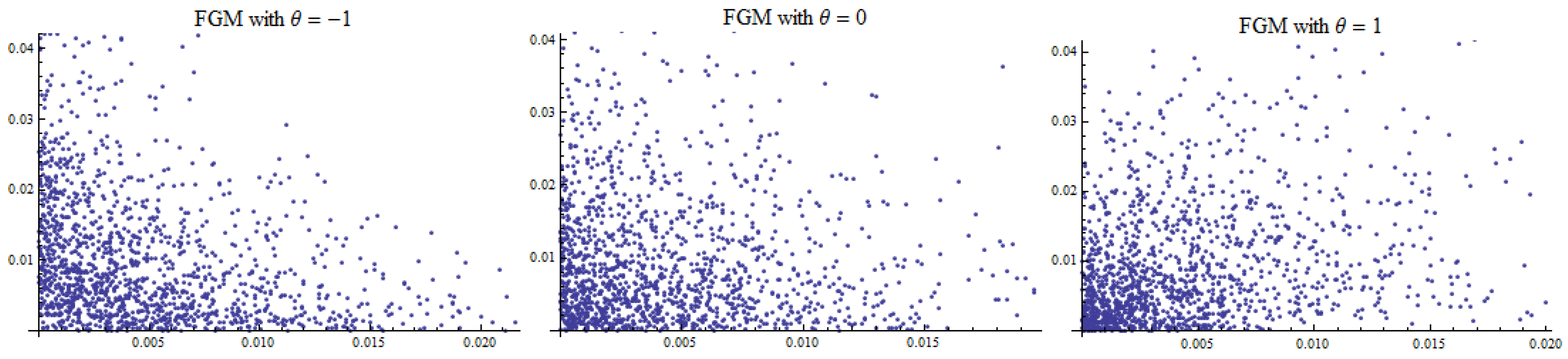
We now present numerical illustration of the Neumann series expression for the first two moments. We start our discussion by presenting the scatter plots of each copula in Figure 1, Figure 2 and Figure 3, where the marginals are exponential distribution, which is in line with the assumptions used in the numerical computations of the moments in this section. All computations were done using Mathematica.

Figure 1. Farlie–Gumbel–Morgenstern (FGM) copula with exponential margins and dependence parameters −1, zero, one.

Figure 1. Farlie–Gumbel–Morgenstern (FGM) copula with exponential margins and dependence parameters −1, zero, one.

Figure 2. Gaussian copula with exponential margins and dependence parameters −1, zero, one.

Figure 2. Gaussian copula with exponential margins and dependence parameters −1, zero, one.

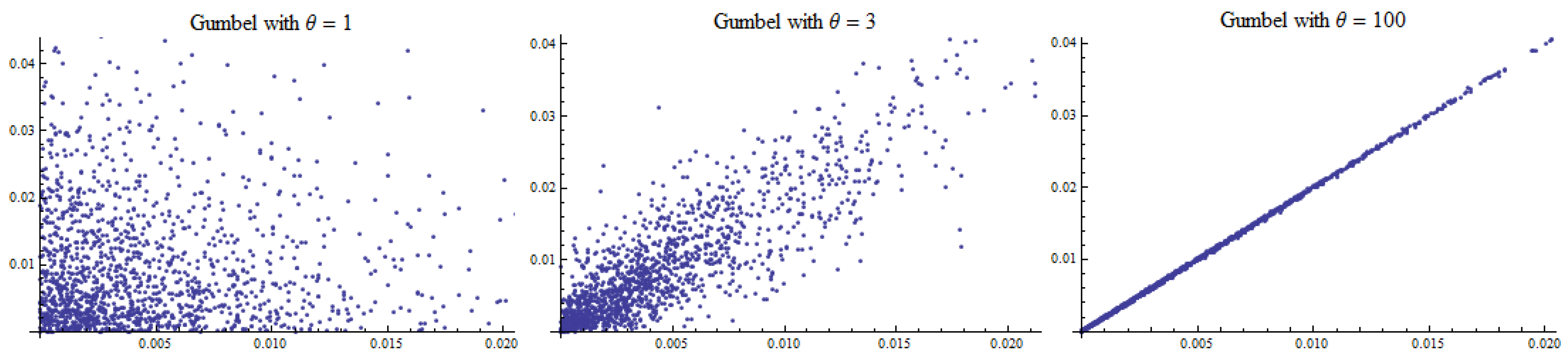
Figure 3. Gumbel copula with exponential margins and dependence parameters one, three, 100.

Figure 3. Gumbel copula with exponential margins and dependence parameters one, three, 100.

4.1. Numerical Accuracy of Neumann Series Expression for Moments

Recall that Equation (16) has at most triple integration involved, while Equation (17) has up to sextuple numerical integration. This implies that the computation of Equation (17) is expected to be close to the solution by [6], due to numerical approximation error, and the values would vary according to selected software packages. To evaluate the performance of the main results, we compare the numerical values returned by our Neumann series (under the column Neumann of Table 1), using the FGM copula, with the numerical values given by the closed form solution in [6] (under the column BCLM of Table 1).

Table 1. Moment verification: the case of the FGM copula. Abs. Dev., absolute deviation; Rel. Dev., relative deviation.

Moment	θ	BCLM	Neumann	Abs. Dev.	Rel. Dev.
${\mu }_Z\left(5\right)$	−0.9	0.475231	0.475231	0	0
	0	0.453173	0.453173	0	0
	0.9	0.431115	0.431115	0	0
${\mu }_Z^{\left(2\right)}\left(5\right)$	−0.9	0.332023	0.329774	0.002249	0.006774
	0	0.287786	0.287786	0	0
	0.9	0.245457	0.247706	0.002249	0.009163

Table 1. Moment verification: the case of the FGM copula. Abs. Dev., absolute deviation; Rel. Dev., relative deviation.

Moment	θ	BCLM	Neumann	Abs. Dev.	Rel. Dev.
${\mu }_Z\left(5\right)$	−0.9	0.475231	0.475231	0	0
	0	0.453173	0.453173	0	0
	0.9	0.431115	0.431115	0	0
${\mu }_Z^{\left(2\right)}\left(5\right)$	−0.9	0.332023	0.329774	0.002249	0.006774
	0	0.287786	0.287786	0	0
	0.9	0.245457	0.247706	0.002249	0.009163

The values in Table 1 were computed using an example of $\delta =0.04$, $\alpha =10$, $\beta =1$, $T=5$ and $\theta =-0.9,0,0.9$. The absolute deviation (Abs. Dev.) figures are obtained by taking the difference between the two columns, BCLM and Neumann (i.e., the absolute value of the solution presented in [6] minus the Neumann series expression), whereas the relative deviation (Rel. Dev.) figures are calculated as $\frac{Abs.Dev.}{BCLM}$.

Our calculations showed that the Neumann series expression for the first moment gives the same value as the closed form solution presented in [6]. On the other hand, the second moment gives a slightly different value at $\theta =-0.9$ and $0.9$, when the r.v.’s, X and W, are highly dependent. After a close scrutiny of the programming messages, we noticed that this is caused by numerical approximation errors of the quadruple, quintuple and sextuple integrations that are not present in the calculation of the first moment. To improve the accuracy of the Neumann series expression for higher order moments, the reader can use other software packages or use Monte Carlo simulation.

4.2. Moments of the Aggregate Discounted Claims

Setting $\delta =0.04$, $\alpha =0.01$ and $\beta =1$ for the case of exponential claim inter-arrival time and exponential claim sizes, respectively, we show the values of moments of the aggregate discounted claims for each copula used in this study. We present the values of the first and second moments of the compound distribution, i.e., ${\mu }_Z\left(5\right)$ and ${\mu }_Z^{\left(2\right)}\left(5\right)$, as well as the variance under each copula in Table 2, Table 3 and Table 4. The term “spread”, which is defined as the difference between the values returned by θ at both ends, i.e., ${\theta }_{-0.95}-{\theta }_{0.95}$ for FGM and Gaussian, and ${\theta }_1-{\theta }_{100}$ for Gumbel, are also shown in Table 2 and Table 3.

Table 2. Values of ${\mu }_Z\left(5\right)$ for various copula.

θ	FGM	θ	Gaussian	θ	Gumbel
−0.95	455.543	−0.95	513.470	1	453.173
−0.9	455.419	−0.9	511.887	5	360.864
−0.5	454.421	−0.5	488.903	15	267.995
0	453.173	0	453.173	30	148.317
0.5	451.926	0.5	409.481	50	104.457
0.9	450.928	0.9	368.612	75	21.486
0.95	450.803	0.95	363.124	100	10.712
Spread	4.74		150.346		431.687

Table 2. Values of ${\mu }_Z\left(5\right)$ for various copula.

θ	FGM	θ	Gaussian	θ	Gumbel
−0.95	455.543	−0.95	513.470	1	453.173
−0.9	455.419	−0.9	511.887	5	360.864
−0.5	454.421	−0.5	488.903	15	267.995
0	453.173	0	453.173	30	148.317
0.5	451.926	0.5	409.481	50	104.457
0.9	450.928	0.9	368.612	75	21.486
0.95	450.803	0.95	363.124	100	10.712
Spread	4.74		150.346		431.687

Our calculations showed that all copula exhibit decreasing values as θ increases, in line with [11]. Intuitively, a negative dependence structure represented by the pair of short inter-claim waiting time (or frequent claim occurrence within a given time period) with huge claim size will only prompt the insurer to charge a higher premium as opposed to the positive dependence structure.

As we have expected, the values of moments do not vary much across θ when calculated under the FGM copula, as opposed to the Gaussian and Gumbel copulas. Being an extreme copula, values of the first moment calculated under the Gumbel copula also showed the widest spread of the first moment.

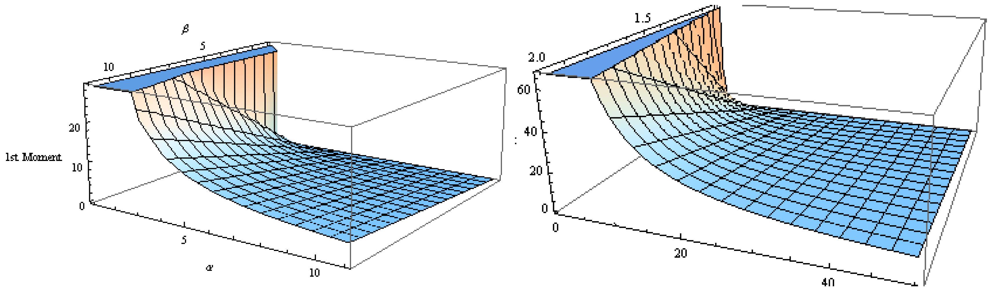
Table 5 shows the values of the first moment as a function of α and β, respectively, for which we use the Gaussian copula at $\theta =-0.9$. It shows that increasing the inter-claim waiting time parameter, β, results in increasing the mean value of the aggregate discounted claims, and vice versa in the case of the claim size parameter. Given an average value of inter-claim arrival time, β, the mean of aggregate discounted claims gets lower as we have a lower average claim size, given by $\frac{1}{\alpha }$. On the other hand, given an average value of the claim size, the mean of the aggregate discounted claims gets bigger as the inter-claim arrival time gets shorter, which implies more frequent claim occurrences. This scenario is illustrated in Figure 4 for $\theta =-0.9$ (left hand side of the diagram), as well as $\theta =0$ (right hand side of the diagram).

Table 3. Values of ${\mu }_Z^{\left(2\right)}\left(5\right)$ for various copula.

θ	FGM	θ	Gaussian	θ	Gumbel
−0.95	336,551.170	−0.95	409,852.140	1	287,784.972
−0.9	332,022.549	−0.9	405,315.216	3	148,590.220
−0.5	312,126.218	−0.5	357,029.617	5	139,437.15
0	287,785.862	0	287,785.862	40	21,804.385
0.5	264,034.461	0.5	212,119.492	75	1,088.013
0.9	245,457.386	0.9	149,988.657	80	229.608
0.95	241,329.490	0.95	136,249.086	100	178.443
Spread	95,221.68		273,603.054		287,606.529

Table 3. Values of ${\mu }_Z^{\left(2\right)}\left(5\right)$ for various copula.

θ	FGM	θ	Gaussian	θ	Gumbel
−0.95	336,551.170	−0.95	409,852.140	1	287,784.972
−0.9	332,022.549	−0.9	405,315.216	3	148,590.220
−0.5	312,126.218	−0.5	357,029.617	5	139,437.15
0	287,785.862	0	287,785.862	40	21,804.385
0.5	264,034.461	0.5	212,119.492	75	1,088.013
0.9	245,457.386	0.9	149,988.657	80	229.608
0.95	241,329.490	0.95	136,249.086	100	178.443
Spread	95,221.68		273,603.054		287,606.529

Table 4. Values of $\mathbf{Var}\left(5\right)$ for various copula.

θ	FGM	θ	Gaussian	θ	Gumbel
−0.95	128,940.627	−0.95	146,200.971	1	82,420.094
−0.9	124,616.083	−0.9	143,286.915	3	13,837.353
−0.5	105,627.773	0.5	118,003.474	5	9,214.320
0	82,420.094	0.	82,420.094	40	5,597.566
0.5	59,797.351	0.5	44,444.803	75	626.365
0.9	42,121.325	0.9	14,113.850	80	112.770
0.95	38,106.145	0.95	4,390.216	100	61.436

Table 4. Values of $\mathbf{Var}\left(5\right)$ for various copula.

θ	FGM	θ	Gaussian	θ	Gumbel
−0.95	128,940.627	−0.95	146,200.971	1	82,420.094
−0.9	124,616.083	−0.9	143,286.915	3	13,837.353
−0.5	105,627.773	0.5	118,003.474	5	9,214.320
0	82,420.094	0.	82,420.094	40	5,597.566
0.5	59,797.351	0.5	44,444.803	75	626.365
0.9	42,121.325	0.9	14,113.850	80	112.770
0.95	38,106.145	0.95	4,390.216	100	61.436

Table 5. Values of ${\mu }_Z\left(5\right)$ under the Gaussian copula at $\theta =-0.9$.

β =1	${\mu }_Z\left(5\right)$	α = 1	${\mu }_Z\left(5\right)$
α = 0.01	511.887741	β = 0.01	0.165673
α = 0.1	51.188786	β = 0.1	0.884887
α = 1	5.118887	β = 1	5.118887
α = 10	0.511838	β = 10	45.911776
α = 15	0.341257	β = 15	67.571651

Table 5. Values of ${\mu }_Z\left(5\right)$ under the Gaussian copula at $\theta =-0.9$.

β =1	${\mu }_Z\left(5\right)$	α = 1	${\mu }_Z\left(5\right)$
α = 0.01	511.887741	β = 0.01	0.165673
α = 0.1	51.188786	β = 0.1	0.884887
α = 1	5.118887	β = 1	5.118887
α = 10	0.511838	β = 10	45.911776
α = 15	0.341257	β = 15	67.571651

Figure 4. Sensitivity of the first moment under the Gaussian copula at $\theta =0$ and $\theta =-0.9$ with respect to claim size and inter-claim time averages.

Figure 4. Sensitivity of the first moment under the Gaussian copula at $\theta =0$ and $\theta =-0.9$ with respect to claim size and inter-claim time averages.

4.3. Premium Calculation under FGM, Gaussian and Gumbel copulas

We now compute the loaded premium related to the risk of an insurance portfolio represented by $Z\left(T\right)$, where the dependence structure is captured by a copula. For that purpose, the first two moments will be useful in the premium calculation based on the expected value principle, the variance principle, as well as the standard deviation (SD) premium principle, as the following:

$$\Pi \left(T\right)=\mathbf{E}\left[Z\right(T\left)\right]+\kappa \mathbf{E}\left[Z\right(T\left)\right]$$

$$\Pi \left(T\right)=\mathbf{E}\left[Z\right(T\left)\right]+\kappa \mathbf{V}ar\left[Z\right(T\left)\right]$$

$$\Pi \left(T\right)=\mathbf{E}\left[Z\left(T\right)\right]+\kappa \sqrt{\mathbf{V}ar\left[Z\right(T\left)\right]}$$

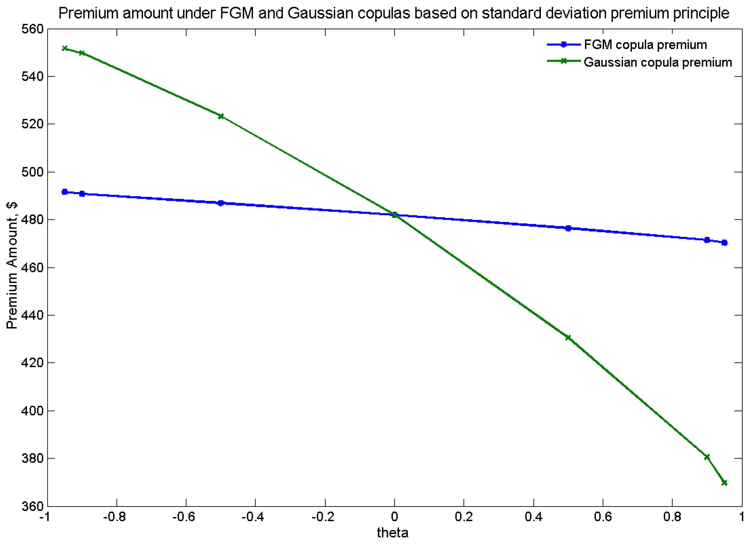
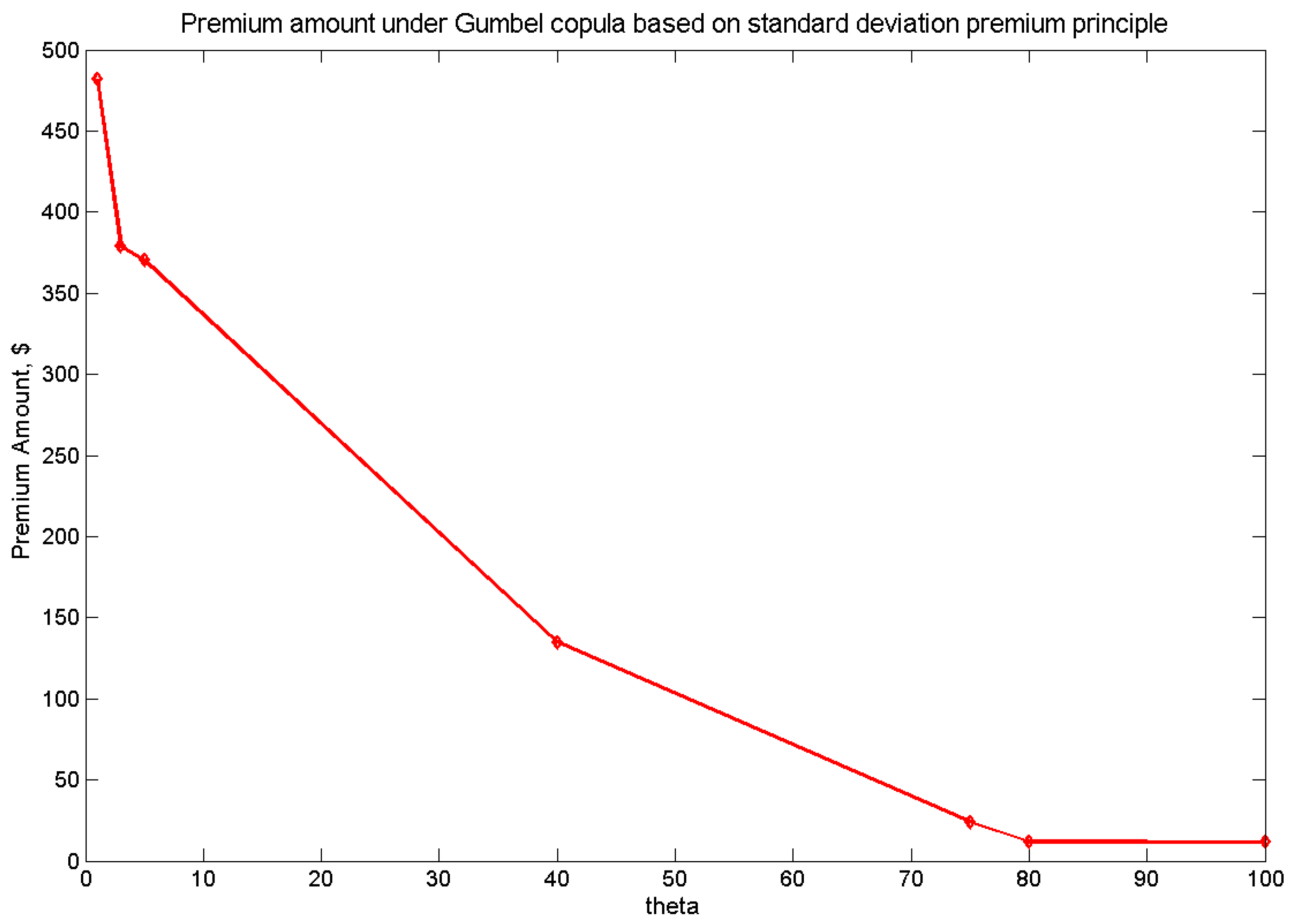
Table 6 exhibits the loaded premium according to the SD principle under the three copulas considered, with $\kappa =0.1$, while Figure 5 and Figure 6 illustrate the range of premiums under the copulas studied according to the SD premium principle.

Table 6. Loaded premium according to the SD principle under various copulas.

θ	FGM	θ	Gaussian	θ	Gumbel
−0.95	491.55	−0.95	551.71	1	481.88
−0.9	490.72	−0.9	549.74	3	378.85
−0.5	486.92	−0.5	523.25	5	370.46
0	481.88	0	481.88	40	134.79
0.5	476.38	0.5	430.56	75	23.99
0.9	471.45	0.9	380.49	80	11.87
0.95	470.32	0.95	369.75	100	11.60
Spread	21.23		181.96		470.28

Table 6. Loaded premium according to the SD principle under various copulas.

θ	FGM	θ	Gaussian	θ	Gumbel
−0.95	491.55	−0.95	551.71	1	481.88
−0.9	490.72	−0.9	549.74	3	378.85
−0.5	486.92	−0.5	523.25	5	370.46
0	481.88	0	481.88	40	134.79
0.5	476.38	0.5	430.56	75	23.99
0.9	471.45	0.9	380.49	80	11.87
0.95	470.32	0.95	369.75	100	11.60
Spread	21.23		181.96		470.28

5. Conclusions

In this paper, we utilized copulas to capture the dependence structure between the inter-claim arrival time and claim sizes in classical actuarial risk theory. To do so, we represented the expression for the $m-th$ order moment proposed in [6,12] in the form of the Volterra integral equation (VIE) of the second kind, which is widely used in renewal theory, demographics, electromagnetism and viscoelasticity.

Figure 5. The loaded premium under FGM and Gaussian copulas based on the SD premium principle.

Figure 5. The loaded premium under FGM and Gaussian copulas based on the SD premium principle.

Figure 6. The loaded premium under the Gumbel copula based on the SD premium principle.

Figure 6. The loaded premium under the Gumbel copula based on the SD premium principle.

We derived the Neumann series expression for this recursive equation using the Picard method of successive approximations, based on which we computed the first two moments of the aggregate discounted claims. For the dependence structure between the inter-claim arrival time and claim sizes, we used a Farlie–Gumbel–Morgenstern copula, a Gaussian copula and a Gumbel copula with exponential marginal distributions. We showed the values of moments of the aggregate discounted claims, as well as the loaded premium for each copula used in this study.

It would be of interest to derive the expression for Equation (2) and Equation (3) using other joint pdfs between X and W. Other copulas with different claim size distributions for X may be considered in the proposed approach, which we leave for further research. We can also consider the Monte Carlo simulation, as well as other numerical methods to solve the VIE (such as Runge–Kutta and the collocation methods), as the next objective of further research to deal with the computation of higher moments.