When the U.S. Stock Market Becomes Extreme?

Abstract

Over the last three decades, the world economy has been facing stock market crashes, currency crisis, the dot-com and real estate bubble burst, credit crunch and banking panics. As a response, extreme value theory (EVT) provides a set of ready-made approaches to risk management analysis. However, EVT is usually applied to standardized returns to offer more reliable results, but remains difficult to interpret in the real world. This paper proposes a quantile regression to transform standardized returns into theoretical raw returns making them economically interpretable. An empirical test is carried out on the S&P500 stock index from 1950 to 2013. The main results indicate that the U.S stock market becomes extreme from a price variation of ±1.5% and the largest one-day decline of the 2007–2008 period is likely, on average, to be exceeded one every 27 years.

1. Introduction

The tail behavior of the financial series has been largely examined by many studies1 with various applications. The key attraction of extreme value theory (EVT) is that it offers a set of ready-made approaches to risk management analysis. A general discussion of the application of EVT to risk management is proposed by [12,15,16]. However, if the oldest studies made use of raw returns (e.g., [9,10] etc.) in their EVT analysis, since then, the literature has applied EVT on independent and identically distributed data such as standardized returns (e.g., [13]). Therefore, many results stemming from EVT applications remain quiet difficult to interpret economically because of the use of these standardized returns and conclusion can be vague. Indeed, the practice is to extract standardized returns by filtering the raw returns with a GARCH family model; then run some standard tests to check for the approximate independent and identically distributed nature of the standardized returns and finally apply EVT on these data. However, these standardized returns have no economic meaning in the real world. In clear, they cannot be understood in terms of monetary units. One naive possibility would have been to apply an OLS procedure to study the relationship between a response variable (raw returns) and an explanatory variable (standardized returns), in order to numerically recompute all the raw returns corresponding to the standardized returns derived from the EVT analysis and forecasting. Recall that the least-squares regression describes how the mean of the response variable changes with the vector of covariates. But standard regression analysis has several limits such as not being robust to extreme observations whereas EVT is based on observations located in the tails. For that reason, this article proposes an empirical methodology to convert the results into monetary units such as stock index returns. This issue seems not to have been addressed previously, perhaps because the typical EVT paper is generally devoted to the sole statistical perspective used to describe the extreme behavior of financial returns, but not to explain the economic meaning. The method is a simple linear transformation of the standardized returns into raw returns using quantile regressions [17]. Quantile regression generalizes the standard regression model to conditional quantiles of the response variable. Hence, it can be be viewed as a natural extension of standard least squares estimation of conditional mean models to the estimation of a series of models for conditional quantile functions [18]. To our best knowledge, no such statistical test has been implemented so far to address this problem of economic interpretation of EVT results. This research is relevant because it gives a new approach for interpreting the EVT results. The main contribution consists in proposing an empirical methodology based on quantile regression for transforming EVT results expressed in the form of standardized returns into raw returns. An application is provided on the U.S. market from 1950 to 2013. The article is organized as follows. Section 2 opens with a brief review of the extreme value theory applications in finance. Section 3 presents an analysis of the data while Section 4 analyses the empirical results. Section 5 summarizes the main findings and concludes.

2. Methodology

2.1. Tail Distribution

A theorem from [19,20] shows that when the threshold u is sufficiently high, the distribution function $F_u$ of the excess beyond this threshold can be approximated by the Generalized Pareto Distribution (GPD):

$$F_u\left(x\right)\approx G_{\xi ,\beta }\left(x\right).$$

(1)

This limit distribution has a general form given by:

$$G_{\xi ,\beta }\left(x\right)=\left\{\begin{array}{cc}1-{(1+\xi x/\beta )}^{-1/\xi },\hfill & \text{for}\xi \ne 0\hfill \\ 1-exp(-x/\beta ),\hfill & \text{for}\xi =0\hfill \end{array}\right.$$

(2)

where $\beta \ge 0$ and where $x\ge 0$ when $\xi \ge 0$ and where $0\le x\le -\beta /\xi$ when $\xi <0$. β is a scaling parameter and ξ is the tail index. The tail index is an indication of the tail heaviness, the larger ξ, the heavier the tail. This distribution encompasses other type of distributions. If $\xi >0$ ($\xi <0$) then it is a reformulated version of the ordinary Pareto distribution and if $\xi =0$, it corresponds to the exponential distribution.

2.2. Threshold Selection

Threshold selection is subject to a trade off between finding a high threshold where the tail estimate has a low bias with a high variance or finding a low threshold where the tail estimate has a high bias with a low variance. Low (high) bias refers to a (non-reliable) reliable estimate for the tail index.

There are two approaches for threshold selection. The first approach is visual inspection and the second one is automatic detection. The first approach of visual selection [16,21,22] denotes a plausible threshold choice based on the results of the two given plot methods, namely, the mean residual life plot and the threshold plot. The mean residual life plot is the first visual method:

$$\left[u,\frac{1}{n_u}\sum _{i=1}^u(x_i-u)\right]$$

(3)

with $n_u$ representing the number of exceedances over the threshold u. The threshold detection begins with a slope is positive. The threshold plot is the second visual inspection method that consists in fitting the GPD over a range of thresholds allowing observation of both the parameter estimate stability and variance:

$$\left[\widehat{\xi },G_{\xi ,\beta }\left(x\right)=1-{(1+\xi x/\beta )}^{-1/\xi }\right].$$

(4)

The second approach, of optimal threshold, corresponds to the application of an automated method which aims at minimizing the Asymptotic Mean Squared Error (AMSE)2. For the optimal threshold selection method, let’s consider an ordered sample of size $n_u$, $X_{n_u}\le ...\le X_1$ with $X_{n_u}$ being the $n_u^{th}$ upper order statistic. The [24] estimator is defined by:

$$\left[n_u,{\widehat{\xi }}_{n_u}^H=\frac{1}{n_u}\sum _{i=1}^{n_u}(log{X}_{n-i+1}-log{X}_{n-n_u})\right].$$

(5)

It has been popular for the optimal threshold to be estimated such that the bias and variance of the estimated Hill tail index vanish at the same rate where the mean squared error is asymptotically minimized. Usually, AMSE is obtained throughout a sub-sample bootstrap procedure. This paper follows [15] who develop a criterion for which the AMSE of the Hill estimator is minimal for the optimal number of observations in the tail. In clear, this approach computes the optimal sample fraction needed to apply the tail index estimator.

2.3. Three Extreme Risk Management Measures

Every day risk management practices require evaluating the potential risk of loss. Three risk management measures can be used to adress this evaluation problem. Most of the recent literature [12,25,26,27,28,29] confirms the superiority of the in and out-the-sample performance of the risk management models when combining a heavy-tailed GARCH filter with an extreme value theory-based approach. For that reason, these three risk management measures are based on returns standardized by GARCH models.

First, the value-at-risk (VaR) is a common risk measure on any portfolio of financial assets with a given probability and time horizon. For example, a one-day 1% VaR of 1 million euros means that there is a 0.01 probability that the portfolio will fall in value by more than 1 million euros over the next day period. However, there is no need to fully identify the probability distribution because only the extreme quantiles are of interest. Therefore, in our setting, the value-at-risk is computed by inverting the tail estimation formula based on the loss distribution:

$$Va{R}_q=u+\frac{\beta }{\xi }\left[{\left(\frac{n_u}{n}(1-q)\right)}^{-\xi }-1\right].$$

(6)

Nevertheless, VaR models have been criticized for their partial inadequacy. First, VaR can be misleading during volatile periods [30,31]. Second, the VaR of a portfolio can be higher than the sum of the respective VaRs of each individual asset in the portfolio [32]. Third, VaR disregards any loss beyond the VaR level.

Second, a complementary measure known as the expected shortfall (ES) is usually used, for example, in margin requirements. ES particularly focuses on the loss beyond the VaR level. It accounts for the size of tail losses since it evaluates the expected loss size given that VaR is exceeded:

$$E{S}_q=Va{R}_q+E\left(X-Va{R}_q|X>Va{R}_q\right)$$

(7)

Third, the return level (RL) [33] highlights the effect of extrapolation, which is useful for forecasting, even if scarcity produces large variance estimates. Let’s consider $x_m$ as the return level that is exceeded on average once every m observations. Let ${\zeta }_u$ be the probability of exceeding the threshold u. Return level is expressed in annual scale so that the N-year return level is the level expected to be exceeded once every N years. From a risk management perspective, RL is a waiting time period before observing a minimum daily loss, while VaR is the minimum daily loss that can occur with a given probability over a certain horizon. Both measures are threfore closed and complementary. $n_{250}$ is the average number of trading days per year with $m=N\times n_{250}$. N-year return level is an average waiting time period. For example, the N-year return level is the level expected to be exceeded once every N years. It comes for the N-year return level:

$$x_m=u+\frac{\beta }{\xi }\left[{\left(N\times n_{250}{\zeta }_u\right)}^{\xi }-1\right]$$

(8)

3. Data Analysis

3.1. Data Description

Let’s define the market log-returns as ${\left\{R_t\right\}}_{t=1,...,T}$ with $T=15,950$ raw daily log-returns computed from closing price of the U.S. S&P 500 stock index. The time period begins on 3 January 1950 and ends on 28 May 2013. When applying EVT analysis, parameters estimates along with standard errors can be quite unreliable. This underlies the importance of having long time-series with an adaptive econometric filter analysis to obtain identically distributed innovations. Indeed, the presence of autocorrelation and hetereskedasticity in log-returns series requires implementing filters for avoiding any type of bias in the analysis since the data need to be independent and identically distributed before applying extreme value theory. Therefore, this study makes exclusively use of filtered data.

3.2. Data Filtering Process

We examine all the possible specifications within five lags. We test 25 specifications of ARMA(p,q) + GARCH(1,1) models with $p=1,...,5$ and $q=1,...,5$. We select the more parsimonious model. Four criteria are used for comparison: the Schwarz criterion, the autocorrelogram of residuals and squared residuals and the ARCH effect test. We take care of the trade off between parsimony and maximizing criteria. We find that the ARMA(1,1) + GARCH(1,1) model produces the best fit. We then test an alternative model, ARMA(1,1) + TGARCH(1,1), that allows for leverage effects by considering the contribution of the negative residuals in the ARCH effect. Finally, the ARMA(1,1) + TGARCH(1,1) specification has the best fit considering the four criteria. The ARMA (1,1) component takes into account the mean reversion nature of the returns, while the TGARCH specification allows for leverage effects by considering the contribution of the negative residuals in the ARCH effect. Table 1 displays the descriptive statistics showing that except the AR(1) term, all the parameters are statistically significant. The AR(1) term was not removed because withdrawing ${\varphi }_1$ did not clearly improved all the criteria. The ARMA(1,1) + TGARCH (1,1) specification is given by:

$$R_t=\mu +{\varphi }_1{R}_{t-1}+{\theta }_1{ϵ}_{t-1}+{ϵ}_t$$

(9)

where the innovations ${ϵ}_t$ being functions of $Z_t$ and ${\sigma }_t$:

$${ϵ}_t=Z_t{\sigma }_t.$$

(10)

The standardized returns $Z_t$ are independent and identically distributed with $Z_t\sim F_Z(0,1)$. The purpose of the time-varying ${\sigma }_t$ is to capture as much of the conditional variance in the residual ${ϵ}_t$ in order to leave $Z_t$ approximately independent and identically distributed:

$${\sigma }_t^2=\omega +\alpha {\left(Z_{t-1}{\sigma }_{t-1}\right)}^2+\gamma {\left(Z_{t-1}{\sigma }_{t-1}\right)}^2{I}_{Z_{t-1}{\sigma }_{t-1}<0}+\beta {\sigma }_{t-1}^2.$$

(11)

Table 1. Descriptive statistics. The Table presents the descriptive statistics of the S&P 500 stock index standardized daily log-returns $\left(Z\right)$ from 3 January 1950 to 31 May 2013. Sample: 15,950 observations.

	Z		Z
Mean	−0.0032	Q5 (residual)	2.9403
		(p-value)	(0.401)
Median	0.0202	Q5 (squared residual)	7.2983 *
		(p-value)	(0.063)
Maximum	7.0191	Q10 (residual)	11.504
		(p-value)	(0.175)
Minimum	−13.1417	Q10 (squared residual)	11.546
		(p-value)	(0.173)
Std. Dev.	1.0001	Q20 (residual)	20.090
		(p-value)	(0.328)
Skewness	−0.5062	Q20 (squared residual)	16.385
(Z-statistic, p-value)	(−16.2613, 2.2×10-16)	(p-value)	(0.566)
Kurtosis	7.8954	μ	0.0002 ***
(Z-statistic, p-value)	(36.6956, 2.2×10-16)	(Z-statistic)	(4.7722)
Jarque–Bera	16607.86 ***	${\varphi }_1$	−0.0812
(p-value)	(0.0000)	(Z-statistic)	(−1.0679)
Engle LM (1)	6.0183 **	${\theta }_1$	0.1853 **
(p-value)	(0.0142)	(Z-statistic)	(2.4722)
Engle LM (2)	6.3745 **	ω	9.37e-07 ***
(p-value)	(0.0413)	(Z-statistic)	(15.5038)
Engle LM (5)	7.2949 *	α	0.0306 ***
(p-value)	(0.1996)	(Z-statistic)	(13.0564)
Engle LM (10)	11.4924	γ	0.0884 ***
(p-value)	(0.3205)	(Z-statistic)	(28.0765)
q1%	−2.5373	β	0.9154 ***
		(Z-statistic)	(415.2990)
q5%	−1.6240	Log-likelihood	54439.85
q95%	1.5658	Akaike criterion	−6.8220
q99%	2.3426	Number	15950

*, ** and *** denotes parameter statistically significant at the 90%, 95% and 99% confidence level. q1%, q5%, q95% and q99% represent the empirical quantile measures at respectively 1%, 5%, 95% and 99%.

Table 1. Descriptive statistics. The Table presents the descriptive statistics of the S&P 500 stock index standardized daily log-returns $\left(Z\right)$ from 3 January 1950 to 31 May 2013. Sample: 15,950 observations.

	Z		Z
Mean	−0.0032	Q5 (residual)	2.9403
		(p-value)	(0.401)
Median	0.0202	Q5 (squared residual)	7.2983 *
		(p-value)	(0.063)
Maximum	7.0191	Q10 (residual)	11.504
		(p-value)	(0.175)
Minimum	−13.1417	Q10 (squared residual)	11.546
		(p-value)	(0.173)
Std. Dev.	1.0001	Q20 (residual)	20.090
		(p-value)	(0.328)
Skewness	−0.5062	Q20 (squared residual)	16.385
(Z-statistic, p-value)	(−16.2613, 2.2×10-16)	(p-value)	(0.566)
Kurtosis	7.8954	μ	0.0002 ***
(Z-statistic, p-value)	(36.6956, 2.2×10-16)	(Z-statistic)	(4.7722)
Jarque–Bera	16607.86 ***	${\varphi }_1$	−0.0812
(p-value)	(0.0000)	(Z-statistic)	(−1.0679)
Engle LM (1)	6.0183 **	${\theta }_1$	0.1853 **
(p-value)	(0.0142)	(Z-statistic)	(2.4722)
Engle LM (2)	6.3745 **	ω	9.37e-07 ***
(p-value)	(0.0413)	(Z-statistic)	(15.5038)
Engle LM (5)	7.2949 *	α	0.0306 ***
(p-value)	(0.1996)	(Z-statistic)	(13.0564)
Engle LM (10)	11.4924	γ	0.0884 ***
(p-value)	(0.3205)	(Z-statistic)	(28.0765)
q1%	−2.5373	β	0.9154 ***
		(Z-statistic)	(415.2990)
q5%	−1.6240	Log-likelihood	54439.85
q95%	1.5658	Akaike criterion	−6.8220
q99%	2.3426	Number	15950

*, ** and *** denotes parameter statistically significant at the 90%, 95% and 99% confidence level. q1%, q5%, q95% and q99% represent the empirical quantile measures at respectively 1%, 5%, 95% and 99%.

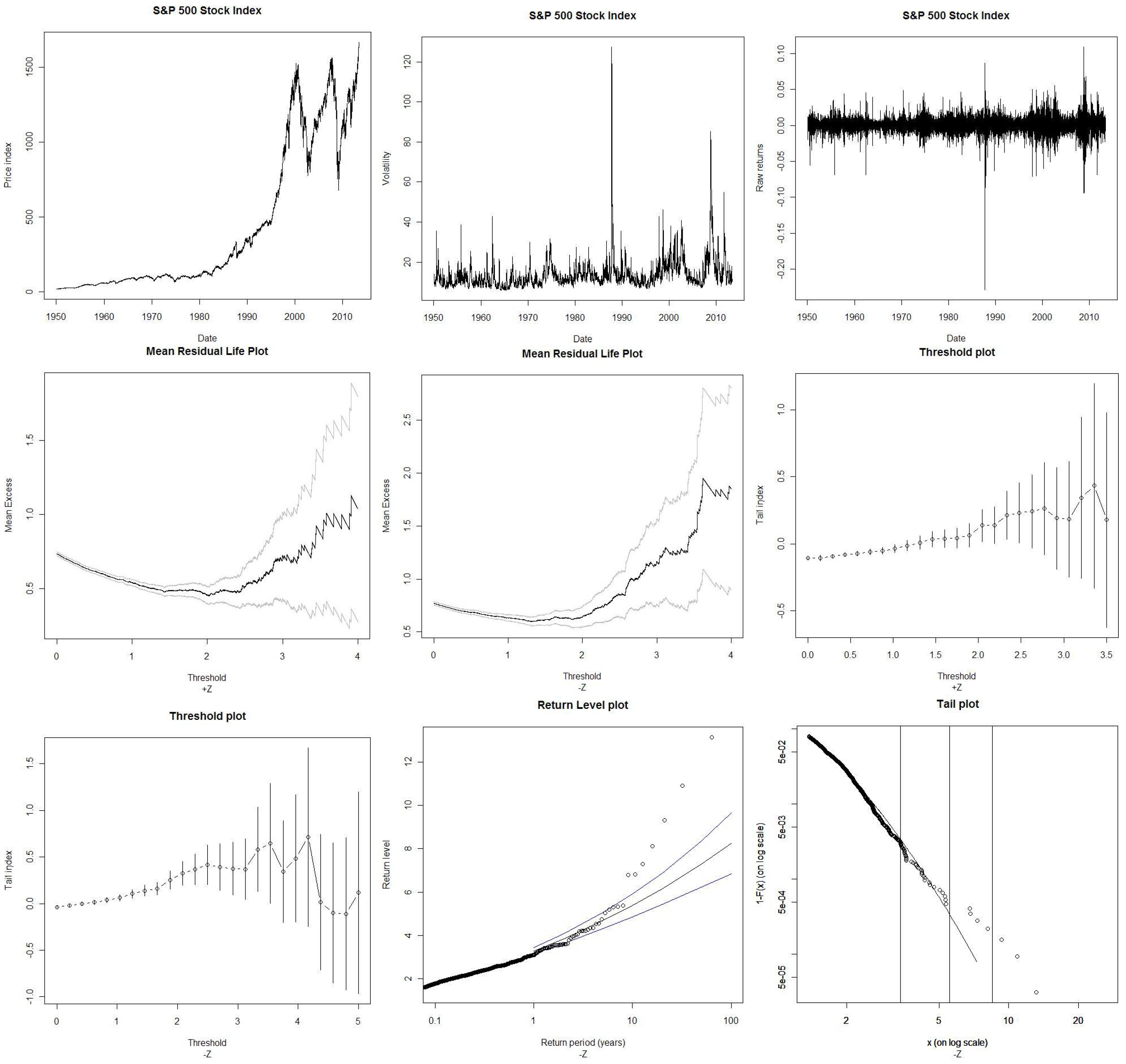
The results for the maximum likelihood estimation of this model are displayed in Table 1. This model provides very good fit according to the selected criteria; all the parameters of the TGARCH(1,1) specification are statistically significant. We therefore extract the maxima and minima from the return shocks ${\left\{Z_t\right\}}_{t=1,...,T}$ corresponding to standardized returns using a time-varying volatility model. Our discussion is hereafter restricted to the standardized (raw) return maxima $+Z$ ($+R$) and minima $-Z$ ($-R$). Figure 1 shows the evolution of the S&P 500 stock index (1) prices; (2) volatility; (3) raw returns and (4) standardized returns.

Figure 1. S&P 500 stock index. The Figure displays graphics from S&P 500 stock index from 3 January 1950 to 28 May 2013. From upper left to lower right corner: The stock index prices. The ARMA(1,1)-TGARCH historical volatility. The raw returns. The next four plots for visual threshold selections from the S&P 500 stock price standardized log-returns. ($+Z$) stands for upper tail and ($-Z$) stands for lower tail. The mean residual life plots are approximately linear with positively sloped, which indicates Pareto behavior overall for the $-Z$ lower tail. The threshold plots display the maximum likelihood estimates for the tail index ξ against a range of thresholds with 95% confidence limits. The stability in the parameter estimates is checked when the parameter estimates are approximately constant above the threshold range. The last two plots display for the lower tail $-Z$, the 100-year return level for the fitted GPD with 95% confidence intervals and tail plot based on a generalized Pareto model fitted to losses over the $-Z$-threshold where the three vertical lines (from left to right) locate the 99%, 99.90% and 99.99% expected shortfall level.

Figure 1. S&P 500 stock index. The Figure displays graphics from S&P 500 stock index from 3 January 1950 to 28 May 2013. From upper left to lower right corner: The stock index prices. The ARMA(1,1)-TGARCH historical volatility. The raw returns. The next four plots for visual threshold selections from the S&P 500 stock price standardized log-returns. ($+Z$) stands for upper tail and ($-Z$) stands for lower tail. The mean residual life plots are approximately linear with positively sloped, which indicates Pareto behavior overall for the $-Z$ lower tail. The threshold plots display the maximum likelihood estimates for the tail index ξ against a range of thresholds with 95% confidence limits. The stability in the parameter estimates is checked when the parameter estimates are approximately constant above the threshold range. The last two plots display for the lower tail $-Z$, the 100-year return level for the fitted GPD with 95% confidence intervals and tail plot based on a generalized Pareto model fitted to losses over the $-Z$-threshold where the three vertical lines (from left to right) locate the 99%, 99.90% and 99.99% expected shortfall level.

3.3. Descriptive Statistics

S&P 500 standardized returns have excess skewness and kurtosis. In all cases, the Jarque–Bera statistics induces a strong rejection of the normality hypothesis. When considering various percentiles from 1% to 99% as a comparison with those implied by the Normal distribution, it shows a clear departure. The Q-statistics, distributed as a ${\chi }_5^2$, ${\chi }_{10}^2$ and ${\chi }_{20}^2$ with 95% critical value, is 11.07, 18.31 and 31.41. The correlogram for the residuals exhibits no more dependence since the Q-statistics for the series are lower than the critical values. The Engle’s Lagrange multiplier test statistic measures the ARCH effect in the residuals; it shows no more evidence of remaining ARCH effects at lag five at the 95% confidence level.

3.4. Quantile Regression

The transformation for recomputing “theoretical raw returns” from standardized returns is very useful for understanding the economic meaning of the statistical inference drawn from EVT results. Indeed, many articles applying EVT to standardized returns leave the reader with few economic interpretations of the results extracted from the filtered series. Therefore, it is important to transform the standardized returns computed from EVT into theoretical raw returns. As recent literature, to our knowledge, does not propose any solution, this article applies a linear transformation based on a semi-parametric technique that extends the ordinary least squares regression model to conditional quantiles. Indeed, standard ordinary least squares modelize the relationship between one or more covariates X and the conditional mean of the response variable Y given X. The quantile regression [17,18] permits a more complete description of the conditional distribution since it generalises the regression model to conditional quantiles of the response variable, such as the 95th or 99th percentile. It appears to be the appropriate approach for the estimation of conditional quantiles of a response variable Y, given a vector of covariates X. Hence, it can be used to measure the effect of covariates, not only in the center of a distribution, but also in the upper and lower tails. Quantile regression is useful when the rate of change in the conditional quantile depends on the quantile. In fact, it can be used with heterogeneous data for which the tails and the center of the conditional distribution vary differently with the covariates. Moreover, it is viewed as a natural extension of OLS estimation with a better consideration brought to extreme observations. It is more robust then OLS because there is no need to do any distributional assumption about the error term, contrary to the normality assumption in the standard regression model. In clear, quantile regression is, by construction, particularly robust to extreme values ([34], p. 7). The linear conditional quantile function can be estimated by solving the following minimization problem:

$${\widehat{\gamma }}_{n_u}\left(q\right)=argmi{n}_{\gamma \left(q\right)}E\left\{{\varsigma }_q\left(Y-X^{\prime }\gamma \left(q\right)\right)\right\}$$

(12)

The check function which weights positive and negative values asymmetrically for any quantile $0<q<1$ is ${\varsigma }_q\left(v\right)=v\left(q-I(v<0)\right)$, where $I(.)$ denotes the indicator function. The vector of coefficients $\gamma \left(q\right)={({\gamma }_{1q},{\gamma }_{2q},...,{\gamma }_{pq})}^{\prime }$ corresponds to p explanatory variables $X={(c,X_1,X_2...X_p)}^{\prime }$ that take the value of the intercept c and the standardized returns Z. Y is the variable of interest corresponding the the raw returns R.

A quantile regression is implemented for the left tail and another one for the right tail. The choice of the percentile level corresponds exactly to the respective selected threshold levels for each tail, which are computed in Section 4.1.

For the left tail (respectively the right tail), the intercept is −0.0032 (respectively 0.0022), the slope coefficient is 0.0084 (respectively 0.0078). The parameters are all statistically significant at the level of 99%. The adjusted $R^2$ value is 0.5978 (respectively 0.6185). Hereafter, any transformation of standardized returns Z into theoretical raw returns $\widehat{R}$ will be computed such as $\widehat{R}=-0.0032+Z\times 0.0084$, $\forall Z<0$, or $\widehat{R}=0.0022+Z\times 0.0078$, $\forall Z>0$.

4. Empirical Findings

4.1. Threshold Selection Results

This article proposes a complete approach for threshold detection mixing visual inspection and automatic detection. The mean residual life plot, in Figure 1, shows that the critical threshold above which the slope is positive is around +1.20 for $+Z$ and −1.40 for $-Z$. According to the threshold plot, a possible range of stability belongs between +0.09 and +1.50 for $+Z$ and between −0.80 and −1.80 for $-Z$. For the optimal threshold detection, we follow [15] who propose a criterion for which the AMSE of the Hill estimator is minimal for the optimal number of observations in the tail. Optimal threshold is around +0.93% for $+Z$ and −1.37% for $-Z$. It corresponds respectively to given number of upper order statistics of 2443 and 1278 observations. The critical threshold values computed from the optimal algorithm respond to the criteria of stability and sufficient exceedances with minimum variance. Table 2 summarizes the results for the threshold selection. Due to the convergence between the three approaches, threshold optimal values are considered in this study.

Table 2. Threshold choice. This Table presents the results for the three approaches for the upper ($+Z$) and lower ($-Z$) tail of the S&P500 stock index standardized log-returns. Visual guidance denotes a plausible threshold choice. Mean residual life plot is the first visual inspection where selection is made around linear region. Threshold plot is the second visual inspection method where selection is made around stability region. The given intervals denote the range of acceptable threshold. The optimal selection method is an automated method consisting in minimizing asymptotic mean squared error.

	$+Z$	$-Z$
Mean residual life plot	+1.20	−1.40
Threshold plot	[+0.09; +1.50]	[−0.80; −1.80]
Optimal selection	+0.9388	−1.3735

Table 2. Threshold choice. This Table presents the results for the three approaches for the upper ($+Z$) and lower ($-Z$) tail of the S&P500 stock index standardized log-returns. Visual guidance denotes a plausible threshold choice. Mean residual life plot is the first visual inspection where selection is made around linear region. Threshold plot is the second visual inspection method where selection is made around stability region. The given intervals denote the range of acceptable threshold. The optimal selection method is an automated method consisting in minimizing asymptotic mean squared error.

	$+Z$	$-Z$
Mean residual life plot	+1.20	−1.40
Threshold plot	[+0.09; +1.50]	[−0.80; −1.80]
Optimal selection	+0.9388	−1.3735

4.2. Tail Characteristics

The critical thresholds of +0.93% for $+Z$ and −1.37% for $-Z$ correspond to the entry point of the right and left tail standardized distribution. These locations in the tail area are relatively closed to those inferred from the raw return series. The transformation from Section 3.4 allows to determine the virtual location entry points for both left and right tail. Indeed, the corresponding critical threshold for the right tail is +0.96% (upper order statistics of 1769) and for the left tail is −1.49% (upper order statistics of 755). This means that approximately beyond ±1.5% price variation, the U.S. stock market enters into a tail area. These thresholds of ±1.5% are the more important results of this study, because they delimit the calm period from the extreme period; they should be analyzed in the light of the associated volatility regime. Indeed, the return–volatility equilibrium requires to examine the stock index returns in the light of the volatility given the asymmetric nature of volatility [35,36,37,38]. In clear, when the market returns go below/beyond these thresholds, we should expect to switch into a different volatility regime. Therefore, let’s consider three volatility regimes corresponding to the raw returns <−1.5%, belonging to the interval −1.5% and +1.5% and >+1.5%. We observe that the average volatility is 22.79% for $\widehat{R}<-1.5\%$, which includes 744 observations in the left tail; it is $12.91\%$ for $-1.5\%<\widehat{R}<+1.5\%$; it is 21.86% for $\widehat{R}>+1.5\%$, which includes 732 observations in the right tail. The volatility level is therefore twice the average level of $12.91\%$ when $\widehat{R}$ is superior in absolute value to 1.5%.

Table 3 displays the results for the GPD when considering the critical threshold values. The maximum likelihood estimators of the GPD are the values of the two parameters ($\xi ,\beta$) that maximize the log-likelihood. The tail index value of $+0.13$ for $-Z$ is positive and statistically significant. The positive sign confirms the presence of fat-tailness for the lower tail $-Z$. The upper tail $+Z$ has a tail index slightly negative, indicating moderate tail behavior corresponding to the Gumbel-type domain of attraction. The scale parameters of $+Z$ and $-Z$ are statistically significant and have the same magnitude.

Table 3. Parameters estimates for the GPD model. Table 3 gives parameter estimates of the general Pareto distribution fitted to the upper ($+Z$) and lower tails ($-Z$) of the S&P500 stock index standardized log-returns. The generalized Pareto distribution is fitted to excesses over the optimal threshold. The vector parameters are estimated by the maximum likelihood method. Nb. Exceedances corresponds to the number of observations in the tail. Percentile is the percentage of observations below the threshold. Neg. Lik is the negative logarithm of the likelihood evaluated at the maximum likelihood estimates.

	$+Z$	$-Z$
ξ	−0.0411 ***	0.1359 ***
(s.e)	(0.0143)	(0.0274)
β	0.5671 ***	0.5168 ***
(s.e)	(0.0140)	(0.0201)
Threshold	+0.9388	−1.3735
Nb. Exceedances	2443	1278
Percentile	0.8468	0.9198
Neg. Lik.	957.047	608.1859

*** denotes parameter significantly different from zero at the 99% confidence level.

Table 3. Parameters estimates for the GPD model. Table 3 gives parameter estimates of the general Pareto distribution fitted to the upper ($+Z$) and lower tails ($-Z$) of the S&P500 stock index standardized log-returns. The generalized Pareto distribution is fitted to excesses over the optimal threshold. The vector parameters are estimated by the maximum likelihood method. Nb. Exceedances corresponds to the number of observations in the tail. Percentile is the percentage of observations below the threshold. Neg. Lik is the negative logarithm of the likelihood evaluated at the maximum likelihood estimates.

	$+Z$	$-Z$
ξ	−0.0411 ***	0.1359 ***
(s.e)	(0.0143)	(0.0274)
β	0.5671 ***	0.5168 ***
(s.e)	(0.0140)	(0.0201)
Threshold	+0.9388	−1.3735
Nb. Exceedances	2443	1278
Percentile	0.8468	0.9198
Neg. Lik.	957.047	608.1859

*** denotes parameter significantly different from zero at the 99% confidence level.

4.3. The Extreme Downside Risk

Table 4 displays some tailed-related risk measures such as the value-at-risk and expected shortfall measures for both Gaussian and General Pareto distributions. Probability level of 99%, 99.5%, 99.9%, 99.95% and 99.99% are considered. The conservative choice of the 99.99% probability level corresponds to a worst possible movement in 10,000 days or approximately 40 years. The reported 0.01%-GPD-VaR is −7.0% and the 0.01%-GPD-ES is −8.49%. The transformation from Section 3.4 indicates that the 0.01%-GPD-VaR and the 0.01%-GPD-ES would respectively represent −6.27% and −7.53% theoretical raw returns. Figure 1 also displays the associate tail plot in log-log scale where the expected shortfall at the level of 99%, 99.90% and 99.99% are visually located; it shows that the GPD largely underestimates these lowest quantiles even the 99.90% level.

Table 4. Value-at-Risk and expected shortfall. Table 4 gives for each probability level of 99%, 99.50%, 99.90%, 99.95%, 99.99% the VaR and the associated expected shortfall estimates based on a (i) GPD model fitted to the S&P 500 stock index negative standardized log-returns ($-Z$) and a (ii) normal distribution.

Probability	VaR-GPD	ES-GPD	VaR-normal	ES-normal
0.9900	−2.6166	−3.4104	−2.3263	−2.6652
0.9950	−3.1151	−3.9873	−2.5758	−2.8919
0.9990	−4.4709	−5.5564	−3.0902	−3.3670
0.9995	−5.1526	−6.3454	−3.2905	−3.5543
0.9999	−7.0068	−8.4912	−3.7190	−3.9584

Table 4. Value-at-Risk and expected shortfall. Table 4 gives for each probability level of 99%, 99.50%, 99.90%, 99.95%, 99.99% the VaR and the associated expected shortfall estimates based on a (i) GPD model fitted to the S&P 500 stock index negative standardized log-returns ($-Z$) and a (ii) normal distribution.

Probability	VaR-GPD	ES-GPD	VaR-normal	ES-normal
0.9900	−2.6166	−3.4104	−2.3263	−2.6652
0.9950	−3.1151	−3.9873	−2.5758	−2.8919
0.9990	−4.4709	−5.5564	−3.0902	−3.3670
0.9995	−5.1526	−6.3454	−3.2905	−3.5543
0.9999	−7.0068	−8.4912	−3.7190	−3.9584

Table 5. Return levels. Table 5 displays the results of the return levels for 1, 2, 5, 10, 20, 50 and 100 years. This table displays the result of the fit of the upper tail ($+Z$) and lower tail ($-Z$) of the S&P500 stock index standardized log-returns. 2× 2 columns represent upper and lower bound with 95% confidence interval.

Period	$+Z$	Lower bound	Upper bound	$-Z$	Lower bound	Upper bound
1	2.8586	2.7746	2.9425	−3.2857	−3.1384	−3.4330
2	3.1921	3.0833	3.3008	−3.8502	−3.6283	−4.0720
5	3.6186	3.4683	3.7689	−4.6829	−4.3138	−5.0519
10	3.9307	3.7426	4.1188	−5.3854	−4.8609	−5.9098
20	4.2340	4.0031	4.4649	−6.1572	−5.4325	−6.8819
50	4.6219	4.3271	4.9166	−7.2958	−6.2255	−8.3661
100	4.9057	4.5577	5.2537	−8.2564	−6.8526	−9.6601

Table 5. Return levels. Table 5 displays the results of the return levels for 1, 2, 5, 10, 20, 50 and 100 years. This table displays the result of the fit of the upper tail ($+Z$) and lower tail ($-Z$) of the S&P500 stock index standardized log-returns. 2× 2 columns represent upper and lower bound with 95% confidence interval.

Period	$+Z$	Lower bound	Upper bound	$-Z$	Lower bound	Upper bound
1	2.8586	2.7746	2.9425	−3.2857	−3.1384	−3.4330
2	3.1921	3.0833	3.3008	−3.8502	−3.6283	−4.0720
5	3.6186	3.4683	3.7689	−4.6829	−4.3138	−5.0519
10	3.9307	3.7426	4.1188	−5.3854	−4.8609	−5.9098
20	4.2340	4.0031	4.4649	−6.1572	−5.4325	−6.8819
50	4.6219	4.3271	4.9166	−7.2958	−6.2255	−8.3661
100	4.9057	4.5577	5.2537	−8.2564	−6.8526	−9.6601

Table 5 displays the return levels for both positive and negative standardized returns with confidence intervals. The return level plot consists of plotting the theoretical quantiles as a function of the return period with a logarithmic scale for the x-axis so that the effect of extrapolation is highlighted. We note that the return levels for negative shocks ($-Z$) are higher in comparison with the positive shocks ($+Z$). Figure 1 additionally shows the associate plot for negative shocks. The 100-year return level is the level expected to be exceeded once every 100 years. It corresponds to a −8.25% standardized return (or −7.33% theoretical raw return) with an asymmetric confidence interval. This asymmetry reflects the greater uncertainty about large values. The 95% confidence interval is obtained from the profile log-likelihood as [−6.85%, −9.66%]. This upper limit of −9.66% is greater in absolute value than the magnitude of the Black Monday standardized return of −9.31%, which is, on average, likely to be exceeded in one every 84 years. As a comparison, the worst standardized return from 2007–2008 financial crisis (−7.31%, 27 February 2007) is, on average, likely to be exceeded in one every 26.5 years (or approximately 27 years) 3.

4.4. EVT with Raw Returns

We apply the EVT methodology directly on raw returns. There is a convergence of the results for extreme identifications but less on extreme predictions. Indeed, the critical thresholds are +1.29% for $+R$ and −1.30% for $-R$, which means that approximately, the S&P 500 stock index becomes extreme from ±1.5% like in the previous section. In addition, concerning the left tail, the 0.01%-GPD-VaR is −7.05% and the 0.01%-GPD-ES is −8.58%. However, we note some differences with the predictions. Indeed, the 100-year return level is −13.62%, which represent a level never reached by the index. The occurence of the Black October crash (19 October 1987, −9.31% with order statistics of 3) is likely, on average, to be exceeded in one every 24.7 years. The occurence of the worst crash from the 2007–2008 financial crisis (22 February 2007, −7.30% with order statistics of 5) is likely, on average, to be exceeded in one every 10.4 years. These predictions are more severe than what is found in Section 4.3.

4.5. Robustness Check

We test the robustness of the methodology that employed EVT combined with quantile regression. We select a sub period (1950–2008) including the financial crisis in order to check for the stability of the parameters. The results are very stable. Indeed, the critical thresholds are +1.16% for $+Z$ and −1.32% for $-Z$, which corresponds to respective theoretical raw returns of +1.21% and −1.39% (or approximately ±1.50%). In addition for $-Z$, the 0.01%-GPD-VaR is −7.05% and the 0.01%-GPD-ES is −8.58%, which corresponds to respective theoretical raw returns of −6.11% and −7.37%. Finally, the 100-year return level is −8.33%, which corresponds to a −7.17% theoretical raw return and the occurrence of the crashes (19 October 1987, 22 February 2007) remains the same.

5. Conclusions

Extreme value theory is usually applied on standardized returns to offer more reliable results, but this makes the economic interpretation more complicated in the real world.

This paper contributes to the literature by proposing an empirical methodology based on quantile regression for transforming EVT results, expressed in the form of standardized returns, into raw returns. This linear transformation converts EVT results in terms of monetary units easy to interpret.

An empirical test on the S&P500 stock index is made from 1950 to 2013. The main empirical results are the following:

First, entering the tail area begins from +0.96% (−1.49%) for the right tail (left tail); in other words, U.S. stock market becomes extreme from a price variation of ±1.5%.

Second, the highest one-day decline from 2007–2008 is likely, on average, to be exceeded one every 27 years versus 84 years for the Black-Monday.

Third, the tailed related risk measures show that the 0.01% GPD VaR/ES correspond to a one-day decline of −6.27%/−7.53%. Future research will extend this methodology to commodity markets given their high level of volatility.

References

- J. Danielsson, and C.G. de Vries. “Tail index quantile estimation with very high frequency data.” J. Empir. Financ. 4 (1997): 241–257. [Google Scholar] [CrossRef]
- J. Danielsson, L. de Haan, L. Peng, and C.G. de Vries. “Using a bootstrap method to choose the sample fraction in tail index estimation.” J. Multivar. Anal. 76 (2001): 226–248. [Google Scholar] [CrossRef]
- J. Danielsson, and Y. Morimoto. “Forecasting extreme financial risk: A critical analysis of practical methods for the Japanese market.” Monet. Econ. Stud. 12 (2000): 25–48. [Google Scholar]
- R. Gencay, F. Selcuk, and A. Ulugulyagci. “High volatility, thick tails and extreme value theory in value-at-risk estimation.” Math. Econ. 33 (2003): 337–356. [Google Scholar] [CrossRef]
- G. Gettinby, C.D. Sinclair, D.M. Power, and R.A. Brown. “An analysis of the distribution of extremes in indices of share returns in the US, UK and Japan from 1963 to 2000.” Int. J. Financ. Econ. 11 (2006): 97–113. [Google Scholar] [CrossRef]
- M. Gilli, and E. Kellezi. Extreme Value Theory for Tail-Related Risk Measure. Working Paper; Geneva, Switzerland: University of Geneva, 2000. [Google Scholar]
- E. Jondeau, and M. Rockinger. “Testing for differences in the tails of stock market returns.” J. Empir. Financ. 10 (2003): 559–581. [Google Scholar] [CrossRef]
- B. LeBaron, and R. Samanta. Extreme Value Theory and Fat Tails in Equity Markets. Working Paper; Waltham, MA, USA: Brandeis University, 2004. [Google Scholar]
- F. Longin. “The asymptotic distribution of extreme stock market returns.” J. Bus. 69 (1996): 383–408. [Google Scholar] [CrossRef]
- F. Longin. “Stock market crashes: Some quantitative results based on extreme value theory.” Deriv. Use Trading Regul. 7 (2001): 197–205. [Google Scholar]
- A.J. McNeil, and T. Saladin. “Developing scenarios for future extreme losses using the POT model.” In Extremes and Integrated Risk Management. London, UK: RISK Books, 1998. [Google Scholar]
- A.J. McNeil. Extreme Value Theory for Risk Managers. Working Paper; Zürich, Switzerland: University of Zurich, 1999. [Google Scholar]
- A.J. McNeil, and R. Frey. “Estimation of tail-related risk measures for heteroskedastic financial time series: An extreme value approach.” J. Empir. Financ. 7 (2000): 271–300. [Google Scholar] [CrossRef]
- K. Tolikas, and R.A. Brown. The Distribution of the Extreme Daily Returns in the Athens Stock Exchange. Working Paper; Dundee, UK: University of Dundee, 2005. [Google Scholar]
- J. Beirlant, Y. Goegebeur, J. Segers, and J. Teugels. Statistics of Extremes: Theory and Applications. Chichester, UK: Wiley, 2004. [Google Scholar]
- P. Embrechts, C. Klüppelberg, and T. Mikosch. Modelling Extremal Events for Insurance and Finance. New York, NY, USA: Springer, 1997. [Google Scholar]
- R. Koenker, and G. Bassett. “Regression quantiles.” Econometrica 46 (1978): 33–50. [Google Scholar] [CrossRef]
- R. Koenker, and K. Hallock. “Quantile Regression.” J. Econ. Perspect. 15 (2001): 143–156. [Google Scholar] [CrossRef]
- A. Balkema, and L. de Haan. “Residual life time at great age.” Ann. Probab. 2 (1974): 792–804. [Google Scholar] [CrossRef]
- J.I. Pickands. “Statistical inference using extreme value order statistics.” Ann. Stat. 3 (1975): 119–131. [Google Scholar]
- S.G. Coles. An Introduction to Statistical Modelling of Extreme Values. London, UK: Springer-Verlag, 2001. [Google Scholar]
- E.J. Gumbel. Statistics of Extremes. New-York, NY, USA: Columbia University Press, 1958. [Google Scholar]
- R. Baillie. “The Asymptotic Mean Square Error of multistep prediction from the regression model with autoregressive errors.” J. Am. Stat. Assoc. 74 (1979): 175–184. [Google Scholar] [CrossRef]
- B.M. Hill. “A simple general approach to inference about the tail of a distribution.” Ann. Stat. 3 (1975): 1163–1174. [Google Scholar] [CrossRef]
- C. Acerbi. “Spectral measures of risk: A coherent representation of subjective risk aversion.” J. Bank. Financ. 26 (2002): 1505–1518. [Google Scholar] [CrossRef]
- K. Inui, and M. Kijima. “On the significance of expected shortfall as a coherent risk measure.” J. Bank. Financ. 29 (2005): 853–864. [Google Scholar] [CrossRef]
- K. Kuester, S. Mittik, and M.S. Paolella. “Value-at-risk prediction: A comparison of alternative strategies.” J. Financ. Econ. 4 (2005): 53–89. [Google Scholar] [CrossRef]
- F.C. Martins, and F. Yao. “Estimation of value-at-risk and expected shortfall based on nonlinear models of return dynamics and extreme value theory.” Stud. Nonlinear Dyn. Econ. 10 (2006): 107–149. [Google Scholar] [CrossRef]
- A. Ozun, A. Cifter, and S. Yilmazer. Filtered Extreme Value Theory for Value-at-Risk Estimation. Working Paper; Kadikoy/Istanbul, Turkey: Marmara University, 2007. [Google Scholar]
- Y. Bao, T.-H. Lee, and B. Saltoglu. “Evaluating predictive performance of value-at-risk models in emerging markets: A reality check.” J. Forecast. 25 (2006): 101–128. [Google Scholar] [CrossRef]
- Y. Yamai, and T. Yoshiba. “Value-at-risk versus expected shortfall: A practical perspective.” J. Bank. Financ. 29 (2005): 997–1015. [Google Scholar] [CrossRef]
- P. Artzner, F. Delbaen, J. Eber, and D. Heath. “Coherent measure of risk.” Math. Financ. 9 (1999): 203–228. [Google Scholar] [CrossRef]
- E.J. Gumbel. “The return period of flood flows.” Ann. Math. Stat. 12 (1941): 163–190. [Google Scholar] [CrossRef]
- X. D’Haultfœuille, and P. Givord. La Regression de Quantile en Pratique. Working Paper; Paris, France: Insee, 2010. [Google Scholar]
- G. Bekaert, and G. Wu. “Asymmetric volatility and risk in equity markets.” Rev. Financ. Stud. 13 (2000): 1–42. [Google Scholar] [CrossRef]
- F. Black. “Studies in stock price volatility changes, American Statistical Association.” In Proceedings of the Business and Economic Statistics Section, Boston, MA, USA, 23–26 August, 1976; pp. 177–181.
- J.Y. Campbell, and L. Hentchel. “No news is good news: An asymmetric model of changing volatility in stock returns.” J. Financ. Econ. 31 (1992): 281–318. [Google Scholar] [CrossRef]
- A. Christie. “The stochastic behavior of common stock variances—Value, leverage, and interest rate effects.” J. Financ. Econ. Theory 10 (1982): 407–432. [Google Scholar] [CrossRef]
- 3Note that for the sake of prudence, the return periods of 84 and 27 years correspond to their respective return level absolute upper bound
© 2014 by the author; licensee MDPI, Basel, Switzerland. This article is an open access article distributed under the terms and conditions of the Creative Commons Attribution license (http://creativecommons.org/licenses/by/3.0/).
Share and Cite
MDPI and ACS Style
Aboura, S. When the U.S. Stock Market Becomes Extreme? Risks 2014, 2, 211-225. https://doi.org/10.3390/risks2020211
AMA Style
Aboura S. When the U.S. Stock Market Becomes Extreme? Risks. 2014; 2(2):211-225. https://doi.org/10.3390/risks2020211
Chicago/Turabian StyleAboura, Sofiane. 2014. "When the U.S. Stock Market Becomes Extreme?" Risks 2, no. 2: 211-225. https://doi.org/10.3390/risks2020211