Tail Risk in Commercial Property Insurance

1
Department of Finance, Imperial College Business School, Imperial College London, LondonSW7 2AZ, UK
2
Civil & Environmental Engineering Department, Faculty of Engineering, Imperial College London, London SW7 2AZ, UK
*
Author to whom correspondence should be addressed.
Risks 2014, 2(4), 393-410; https://doi.org/10.3390/risks2040393
Submission received: 6 April 2014
/
Revised: 26 July 2014
/
Accepted: 30 July 2014
/
Published: 29 September 2014
(This article belongs to the Special Issue Risk Management Techniques for Catastrophic and Heavy-Tailed Risks)
Abstract
:We present some new evidence on the tail distribution of commercial property losses based on a recently constructed dataset on large commercial risks. The dataset is based on contributions from Lloyd’s of London syndicates, and provides information on over three thousand claims occurred during the period 2000–2012, including detailed information on exposures. We use occupancy characteristics to compare the tail risk profiles of different commercial property exposures, and find evidence of substantial heterogeneity in tail behavior. The results demonstrate the benefits of aggregating granular information on both claims and exposures from different data sources, and provide warning against the use of reserving and capital modeling approaches that are not robust to heavy tails.
1. Introduction
Property and business interruption risks represent roughly a third,1 or USD 175 billion, of direct insurance premiums written in commercial insurance lines worldwide (see [1]). The latter also include liability insurance, commercial auto insurance, and specialty lines such as off-shore energy and workers’ compensation.2 Property insurance typically includes fire insurance, which offers protection against fire and lightning, but may also provide additional cover against natural and social perils such as wind, flood, and vandalism. Business interruption is a complementary insurance covering the expenses and losses incurred when business is interrupted and damages are being repaired. The demand for commercial property insurance is dominated by medium and large corporations that need to insure complex, high severity risks. The largest property insurance markets in the world are the US3 and the UK.4
Despite their relevance for the corporate sector and (re)insurers operating in commercial insurance lines, large commercial property risks are poorly understood. This is due to the limited public information available on property losses and exposures, the heterogeneity of risk characteristics of insured values, and the complex relation between hazard events and realized losses, as small events may often precipitate major disasters. These factors make it difficult for insurers to build reliable statistical claims information, whereas companies that have larger insurance portfolios and more sophisticated claims reporting systems have no incentive to disclose information for competitive reasons. The literature on the subject is scant. The few methodological contributions available emphasize the challenges of pricing high layers of exposure, and offer insights into the blending of exposure and experience rating (see [2,3,4]). As a result, the insurance industry is overly reliant on underwriters’ judgment and recent claims history, and finds it difficult to properly understand the true risk that it is taking on. On the demand side, the excessive weight placed on reported claims and the variability of pricing schedules across exposures result in a considerable degree of price volatility, which makes it challenging for corporates to budget for insurance purchases on a systematic basis.5
In this paper, we shed some light on the tail distribution of commercial property risks by using a recently constructed dataset on large commercial risks. This new data source is based on information collected from two leading Lloyd’s syndicates writing a total of GBP 2.67bn gross premiums across all lines of business in 2012, a figure representing around 10% of Lloyd’s gross premiums that year. As Lloyd’s is predominantly a subscription market, the claims information provided by the two syndicates allows us to encompass a substantially larger fraction of business transacted, making the dataset representative of the business written in the London market.6
To measure the tail risk of commercial property exposures, we use a parsimonious model based on approximating the tail behavior of the claims with a power law. In particular, we estimate the tail index, a parameter describing how fast the tail of a power law decays: the lower the tail index, the greater the probability mass in the tails. To ensure robustness relative to small sample bias, heterogeneity, and dependence of the claims considered, we resort to the log-log rank-size method, as presented by Gabaix and Ibragimov [6], and discussed more in detail in Section 3 below. As a robustness check, we also apply the method of Huisman et al. [7], which is designed to address small sample issues (see Section 3.3 for a review of alternative approaches). Estimation of the tail index offers immediate insights for pricing, reserving, and capital modeling exercises. In particular, the value of the tail index is in one-to-one correspondence with the maximal order of finite (centered) moments of the risks considered. For example, the skewness only exists for values of the tail index strictly larger than three; the variance only exists for values strictly larger than two; and the mean only exists for values strictly larger than one (e.g., [8,9]). The tail index can be regarded as being infinite for Normal distributions, as the tail decay is faster than exponential, and moments of an arbitrary order are then finite. In our data, we find that commercial property risks are significantly heavy tailed. For several rating factor configurations, the hypothesis of existence of the variance can be rejected at the 5% significance level. For some important classes of risk, even the hypothesis of existence of the mean can be rejected.7
Existence of a finite variance is essential for the application of standard statistical methods, such as least squares methods. It is also crucial for reserving methods based on risk margins proportional to the standard deviation of the claims,8 meaning that such methods are inappropriate for liabilities modeled by extrapolating available claims information far into the tails. Existence of a finite mean is important for capital modeling and quantile-based risk measures, such as Value at Risk (VaR) in the Solvency II framework. In particular, coherence of VaR as a risk measure in the sense of Artzner et al. [13] may be violated, meaning that the diversification benefits on which a subscription market like Lloyd’s is based may be limited for some classes of commercial property risks. As an example, denote by the random variable the risk exposure resulting from retaining fractions (with , ) of i.i.d. risks . If the risks belong to the class of stable distributions with tail index α, for example, it can be shown that for tail probability parameter and tail index value (see [14,15]). Regulators should therefore be aware of the risk concentration incentives that may arise from commercial property exposures. Similarly, (re)insurers should tread carefully with high layers of exposure in that space, as internal capital charges may underestimate the true risk being taken on.
On the methodological side, we need to deal with potential issues arising from the structure of the data. Although our dataset is large relative to extant data sources,9 we are still faced with small sample estimation challenges, in particular when conditioning on relevant rating factors. Moreover, the observed losses may have a dependence structure induced by the underwriting strategies pursued by the syndicates during the sampling period. We address these issues by using the log-log rank-size regression method with the optimal rank shift indicated by Gabaix and Ibragimov [6]. As demonstrated by these authors, their adjustment optimally reduces the bias arising in small samples, and delivers estimates robust to the presence of heterogeneity and dependency in the data, including common factors. For comparison, we pair this method with the popular Hill [17] estimator, and the weighted-Hill estimator of Huisman et al. [7], which was specifically designed to address small sample issues. The results allow us to reject the hypothesis of existence of first or second moments at a good significance level in some interesting cases. Finally, we explore the relative contribution of different rating factors to tail risk, by expressing the tail index as a deterministic function of relevant covariates, and adopting a regression approach in line with Beirlant et al. [18], Beirlant and Goegebeur [19], and Wang and Tsai [20].
The paper is organized as follows. In the next section, we provide details on the dataset. In Section 3, we outline the statistical methodologies used. In Section 4, we provide tail estimation results for some configurations of exposure characteristics. Section 5 concludes, offering recommendations for future research.
2. Data
The Imperial-IICI dataset contains claim and exposure information obtained from two leading syndicates of Lloyd’s of London. As the latter is a subscription market, the data span business written by a number of other syndicates. Granular information on claims and exposures was obtained from brokers’ submissions. These are documents informing the ‘lead’ underwriter of any claims occurring under a policy; the information is then shared with the market, in order to allocate the losses to each ‘follower’, depending on the individual retentions of the syndicates that co-insured the risk underwritten by the ‘lead’. Brokers’ submissions are fundamental in our analysis, as they allow us to determine claims from the ground up (FGU). It is in general very difficult to recover FGU claims from the losses incurred by individual syndicates, due to the complex layering and coinsurance arrangements characterizing large commercial property insurance. All data were anonymized and aggregated by using fictitious claims and policy identifiers. Internal validation of the data was carried out by looking at individual claims narratives and policy schedules, which are documents listing the asset values insured under a policy. External macro-validation was carried out by using data from fire protection agencies as compiled by ISO Verisk.10
The Imperial-IICI FGU claims provide aggregate information on indemnities for physical damage and business interruption, as well as claims assessment and settlement fees. Both claims and exposures are expressed in 2012 USD terms;11 the normalization is obtained by trending claims and exposures at an average rate of 2.5% per annum across the two syndicates. An example of data record is presented in Table 1. The record reports location information, and classifies the risk type according to the Lloyd’s risk codes (a selection of these codes is presented in Table 2). The claim can be further understood by using occupancy type information, which has three levels of increasing granularity. The first one broadly classifies exposures into commercial (e.g., offices, banks, stores), manufacturing (e.g., utilities, food processors, mines), and residential property (e.g., hotels, hospitals). The second level provides some more detail according to the definitions reported in Table 3, allowing one to distinguish, for example, a hotel from a hospital, or metals from food producers. The third occupancy level offers a more granular view of the exposures, distinguishing for example between large vs. small hotels, heavy vs. light fabrication infrastructure, and food & drugs vs. chemicals vs. metal & minerals processing plants. Finally, occupancy information is complemented by the claim narrative, which may also provide some indications on the hazard event (e.g., burst of waterpipe, electrical failure, fire from hotel restaurant).
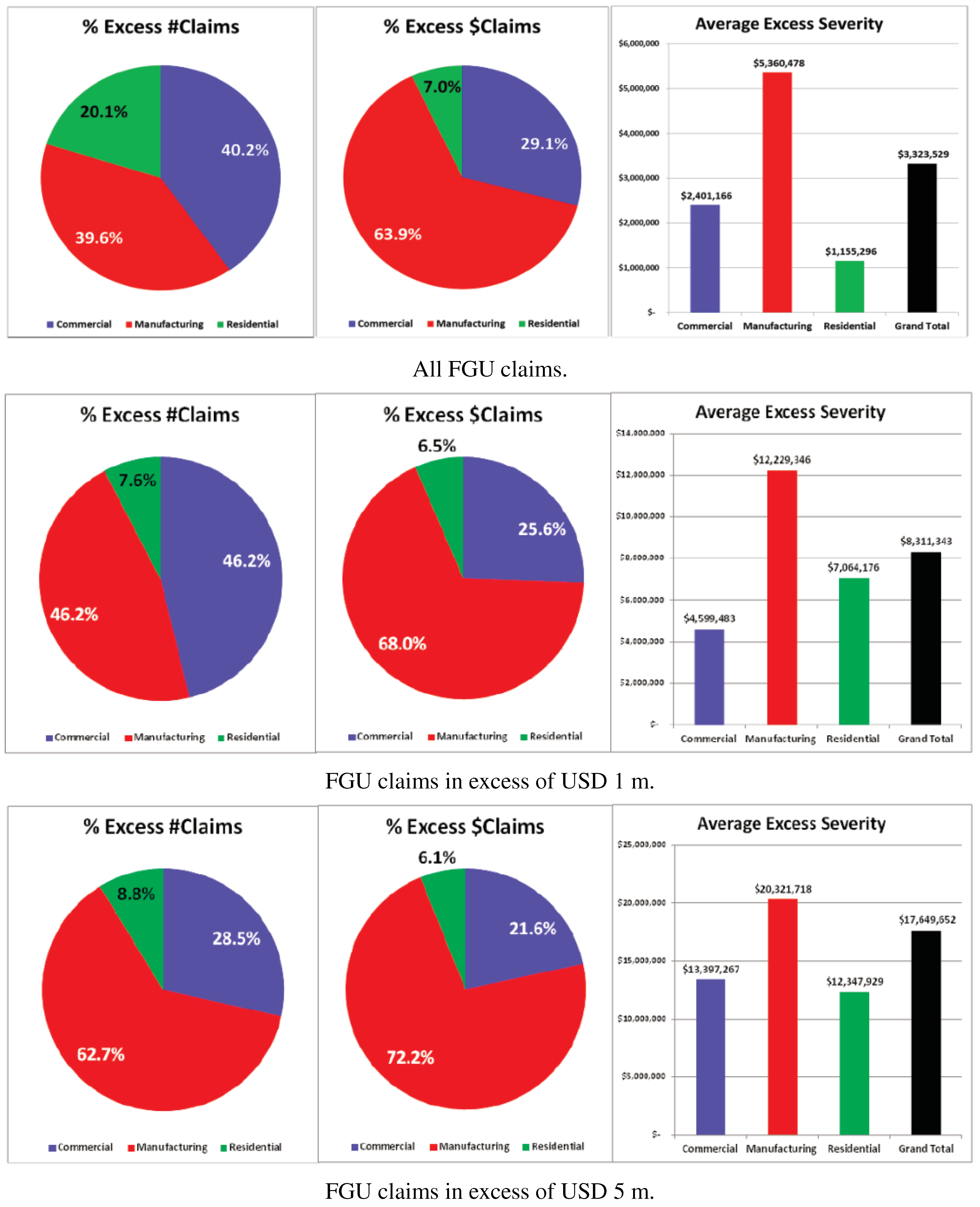
Table 4 gives an idea of the geographical distribution of the losses. Although the dataset has global scope, the largest subsample is represented by North American data. The Worldwide data class is currently being analyzed at a deeper level, and might result in the allocation of claims to more precise locations in the future. In Figure 1, we give an idea of the claim counts and average FGU losses in excess of different thresholds. Information on claim counts by year and occcupancy level 2 information is reported in Table 5.

| Region | Country | Risk Code | Occupancy 1 | Occupancy 2 | Occupancy 3 |
|---|---|---|---|---|---|
| NoA | US | P2 | RE | R | 51 |
| (Physical damage; primary layer property; USA; excluding binders) | (residential) | (residential) | (Large Hotels) |
| Risk Code | Definition |
|---|---|
| B2 | Physical damage; private property; USA; binder |
| B3 | Physical damage; commercial property; USA; binder |
| B4 | Physical damage; private property; excluding USA; binder |
| B5 | Physical damage; commercial property; excluding USA; binder |
| P2 | Physical damage; primary layer property; USA; excluding binders |
| P3 | Physical damage; primary layer property; excluding USA; excluding binders |
| P4 | Physical damage; full value of property; USA; excluding binders |
| P5 | Physical damage; full value of property; excluding USA; excluding binders |
| P6 | Physical damage; excess layer property; USA; excluding binders |
| P7 | Physical damage; excess layer property; excluding USA; excluding binders |
| PG | Operational power generation, transmission, and utilities; excluding construction |
| Code | Definition | Code | Definition |
|---|---|---|---|
| A | Miscellaneous | Q | Offices/Banks |
| B | Manufacturers/Processors | R | Residential |
| C | Chemicals/Pharmaceuticals | T | Transport |
| D | Bridges/Dams/Tunnels/Piers | U | Utilities |
| E | Conglomerates | V | Telecoms and Data Processing |
| F | Food | W | Woodworkers (Sawmills, Papermills) |
| G | Grain | X | Onshore Crude |
| H | General Mercantile/Shops | Y | Onshore GasPlants |
| J | Mines | Z | Onshore Construction |
| K | Crops | 2 | Hospital/Health care centres |
| L | Auto | 4 | Semiconductor/Fabs |
| M | Metals | 5 | Motor Manufaturers |
| O | Municipal Property | 6 | Warehouses |
| P | Energy (Oil Refineries/Petrochemicals) |
| Lloyd’s Code | Description | |
|---|---|---|
| AF | Africa | 22 |
| AS | Asia - Pacific | 54 |
| CA | Central Asia | 21 |
| EU | Europe | 78 |
| LA | Latin America - Carribean | 78 |
| ME | Middle East | 13 |
| NA | North America | 1576 |
| OC | Oceania | 71 |
| WW | World Wide | 1258 |
| Total | 3171 |
Figure 1.
Claims breakdown by Occupancy Level 1 and by excess FGU above different thresholds.

| Years | RE | CO | MA |
|---|---|---|---|
| 2000 | 5 | 116 | 69 |
| 2001 | 20 | 110 | 58 |
| 2002 | 17 | 97 | 92 |
| 2003 | 69 | 105 | 138 |
| 2004 | 41 | 96 | 112 |
| 2005 | 12 | 129 | 89 |
| 2006 | 22 | 74 | 55 |
| 2007 | 143 | 105 | 153 |
| 2008 | 51 | 76 | 100 |
| 2009 | 154 | 55 | 83 |
| 2010 | 110 | 97 | 108 |
| 2011 | 23 | 60 | 51 |
| 2012 | 2 | 4 | 0 |
| Total | 669 | 1124 | 1108 |
3. Methodology
We use a simple yet effective method to estimate the tail index, which relies on the log-log rank-size (LLRS) OLS regression. The method is severely biased in small samples and has often been applied with an incorrect formulation for the standard errors. We apply the optimal bias correction and the correct formula for the standard errors indicated by Gabaix and Ibragimov [6]. Application of the method with an optimal ranks shift is very robust to heterogeneity and dependence of the data, including common factor structures. For comparison, we pair the method with the popular Hill estimator, which suffers from significant bias in small samples, and with the weighted Hill estimator developed by Huisman et al. [7] to deal with small sample issues. Readers interested in the empirical results may skip the next sections and go directly to Section 4.
3.1. Hill Estimator.
Hill [17] proposed a simple method for estimating the tail index from a sequence of i.i.d. observations. Let denote the i-th order statistic of losses, such that for , with n the size of the sample. Let us focus on the losses in excess of the k-th order statistic, and assume a conditional Pareto distribution for the random loss L in excess of the threshold . We have
where is the tail index and C a positive constant. The Hill estimator for the parameter is the maximum likelihood estimator
The standard error for the Hill estimate of the tail index, , is . To understand the bias affecting Equation (1) in small samples, consider the class of distribution functions (see [21,22]):
for positive parameters , and real (the case and corresponding to a Pareto distribution). Dacorogna et al. [22] showed that the above is the second order expansion of the cumulative distribution function of a vast class of heavy tailed distributions, and provided the following approximations for the expected value and variance of the estimator in Equation (1):
for and going to infinity. The above show how the choice of threshold introduces an important trade-off between bias and efficiency.
3.2. LLRS Regression
A popular alternative to more complex estimators for the tail index is to run the OLS regression
with . The tail index is given by the OLS estimator . The procedure is typically applied with , hence the name LLRS. Unfortunately, this approach is strongly biased in small samples, as can be seen from the following asymptotic expansions for the OLS estimator (see [6]):
where denotes a standard Normal random variable. When using the LLRS method, one should therefore apply the optimal rank shift . We will refer to this case as the LLRS-1/2 method. The relevant standard error of the OLS estimator of the slope coefficient is then given by ; again, we refer to Gabaix and Ibragimov [6] for a discussion of this result.
3.3. Alternative Methodologies
There are several alternative methods to estimate the tail index or its inverse.12 As a robustness check, we consider the method proposed by Huisman et al. [7] to deal with small samples, and the bias-efficiency trade-off formalized in Equation (2). Huisman et al. [7] note that, for small enough k, the bias can be approximated by a linear function, suggesting the use of the regression
They then compute Hill estimates for different values of , where the upper bound is the largest value for which the linear approximation of holds, and use the resulting vector of ’s to estimate the parameters of (3). As k goes to zero, the intercept in (3) provides an unbiased estimate of the parameter γ. Note that and cannot be estimated by OLS for two reasons. First, from Equation (1) we see that the variance of depends on k, and hence the error term is heteroskedastic. Second, for all , the estimators and are correlated. Huisman et al. [7] therefore use Weighted Least Squares (WLS) combined with an appropriate method to compute the standard errors to deal with the overlapping data problem. They obtain the following weighted Hill estimator,
where we refer to Huisman et al. [7] for details on the weights .
4. Empirical Evidence
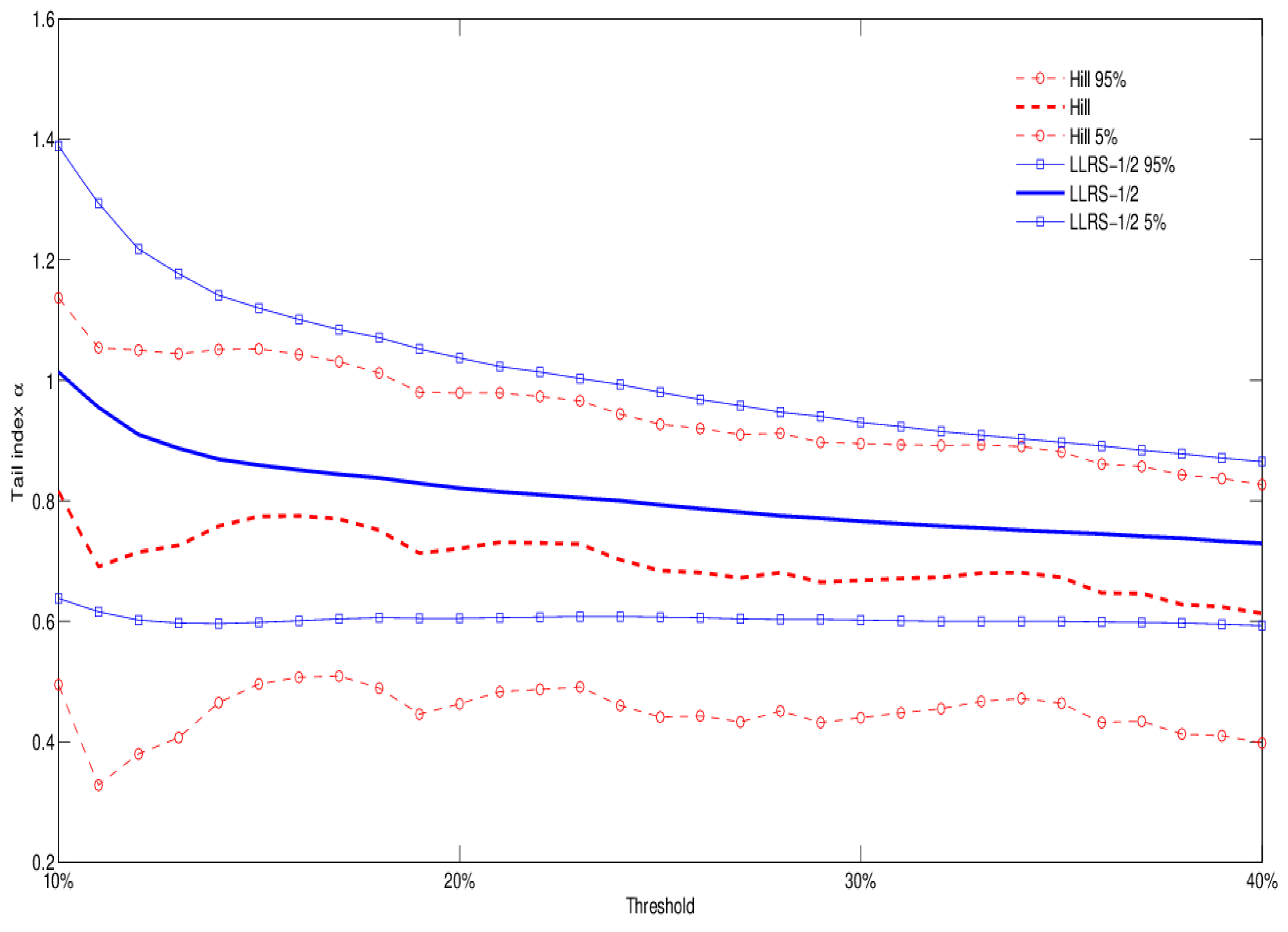
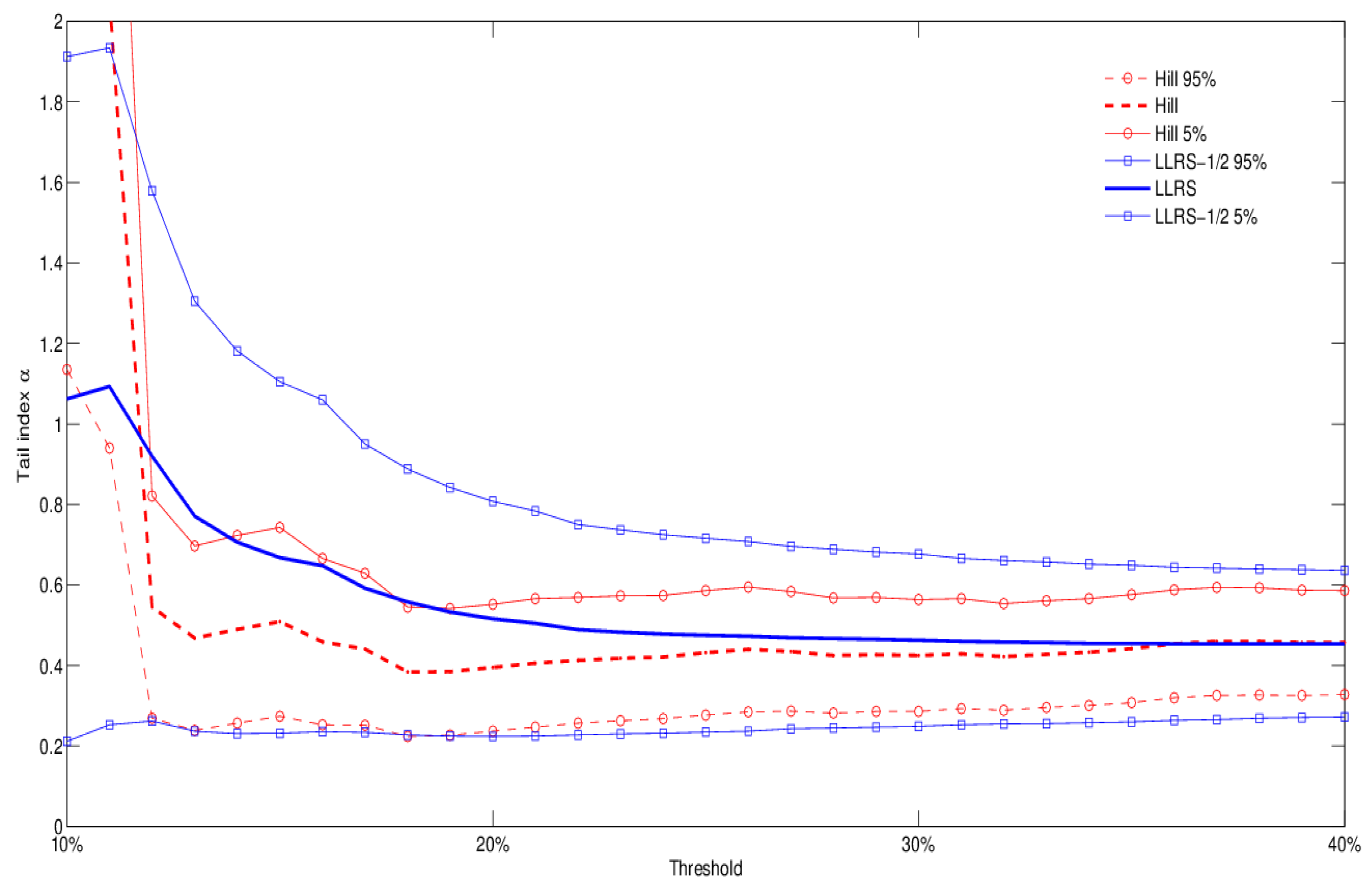
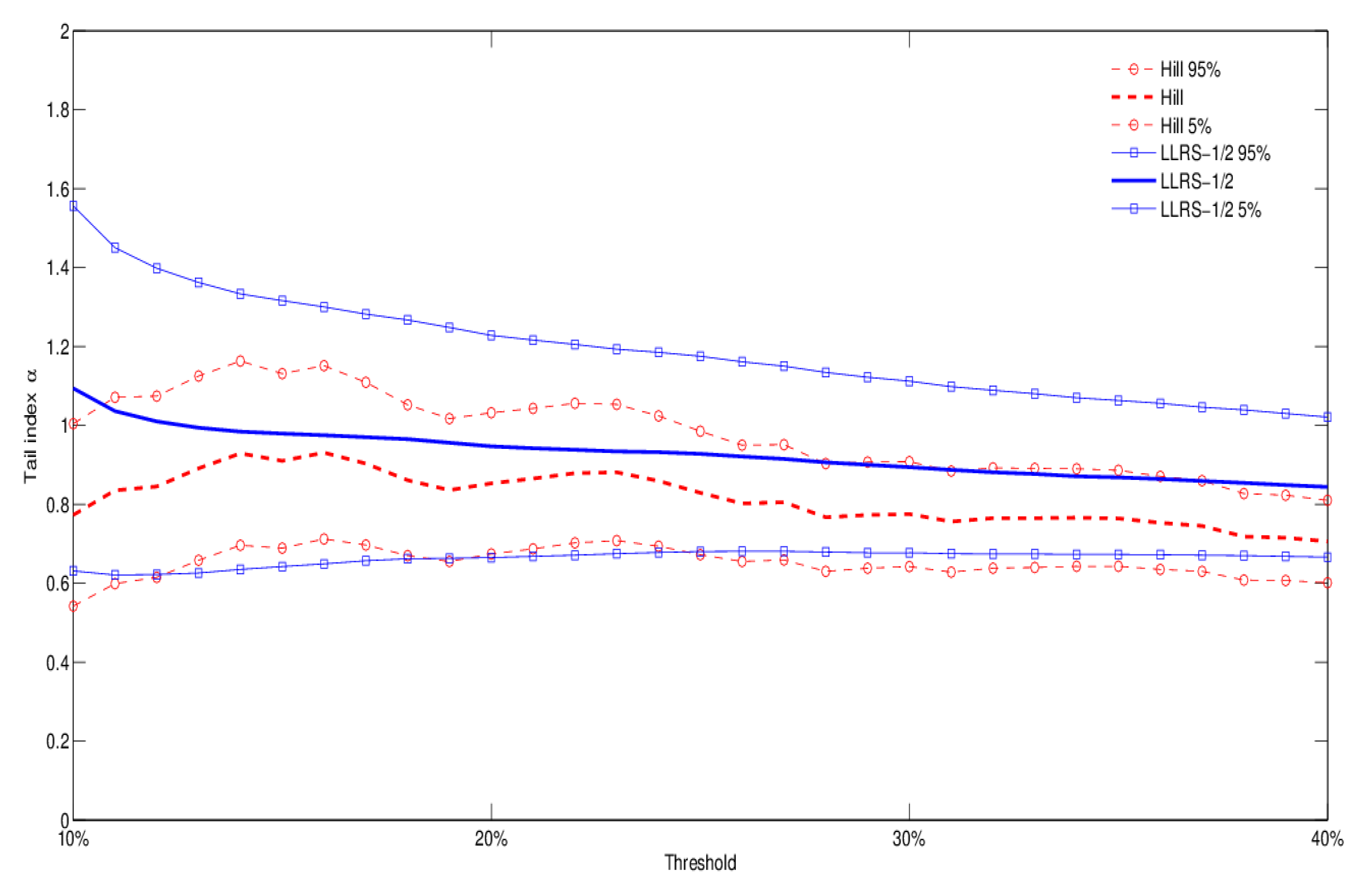
In this section we provide tail index estimates for the subset of the Imperial-IICI dataset covering commercial property claims and exposures.13 Let us first provide a comparison of the two estimation methods outlined in Section 3.1–Section 3.2 by looking at property exposures classified as RE (residential) according to Occupancy Information Level 1. These include hotels, condos, and municipal property such as council houses, universities, and colleges. Figure 2 reports tail index estimates and 90% confidence bands for the Hill and LLRS-1/2 methods. Estimates are based on subsamples obtained by considering between 10% and 40% of the largest losses. The results suggest considerable heaviness of the tail distribution: both estimation methods indicate a tail index close to one; the existence of a finite variance can be rejected at the 5% significance level.
Figure 2.
Tail index estimates and 90% confidence bands for Occupancy Level 1 RE (residential): comparison of Hill and LLRS-1/2 regression methods for different estimation thresholds (from 10-th to 40-th percentile of the data).
Figure 2.
Tail index estimates and 90% confidence bands for Occupancy Level 1 RE (residential): comparison of Hill and LLRS-1/2 regression methods for different estimation thresholds (from 10-th to 40-th percentile of the data).

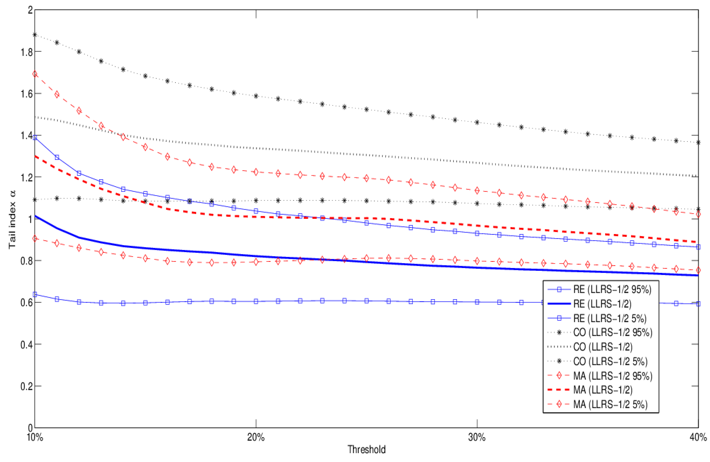
To demonstrate the importance of occupancy type, we then compare the tail behavior of Occupancy Information Level 1 types RE (residential), CO (commercial), and MA (manufacturing). Figure 3 depicts the results obtained with the LLRS-1/2 method. They indicate considerable variation in tail behavior across occupancy types. Based on our data, in particular, all types have tail indices lower than two at the 95% confidence level; commercial losses have the highest tail index estimates, residential losses the lowest, whereas manufacturing claims are somewhere in the middle. Although losses in our dataset are on average substantially larger for manufacturing than residential exposures, the results suggest that the latter may be more dangerous from a distributional perspective. We must bear in mind, however, that residential exposures are underrepresented in our dataset, as shown for example in Figure 1. As a robustness check, in Table 6 we report the results obtained by applying the method of Huisman et al. [7] to the three occupancy types. The results show broad agreement with the LLRS-1/2 method, in particular for MA and CO exposures.
Figure 3.
Tail index estimates and 90% confidence bands (LLRS-1/2 regression method) for all Occupancy Level 1 types (CO, MA, RE).
Figure 3.
Tail index estimates and 90% confidence bands (LLRS-1/2 regression method) for all Occupancy Level 1 types (CO, MA, RE).

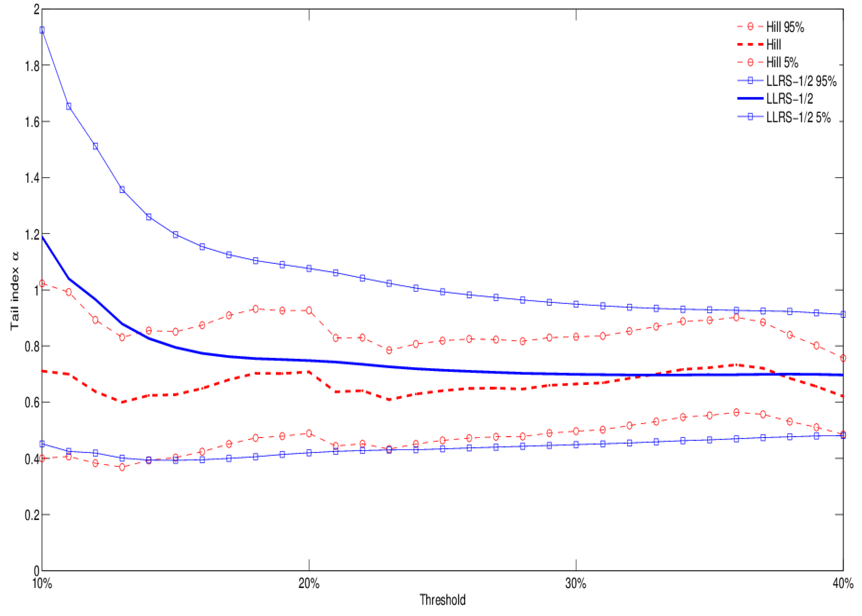
The use of Occupancy Information Level 3 gives us the opportunity to explore variations in tail behavior within a specific occupancy class. Let us consider RE (residential) exposures, for example, and distinguish between Large Hotels and Dwellings, the latter including condos, housing associations, and institutional housing. Figure 4 and Figure 5 show that the second type of exposures is lighter tailed than Large Hotels. We report results for both the Hill and LLRS-1/2 estimation methods, which provide similar implications. It is well known that hotel exposures have different risk profiles, depending for example on the presence of a restaurant (increasing the risk of fire), and may be more or less risky than condos and apartment complexes. Although the dataset does not allow us to explore this dimension at the moment (including the presence of sprinklers), our results suggest that the Large Hotels occupancy class may subsume the presence of serious sources of risk (such as restaurants), thus explaining the lighter tail behavior of Dwellings. Finally, in Figure 6 we report the tail index estimates for the case of aggregate Occupancy Level 2 types C (chemicals), J (metals), and M (mines). Again, the results show considerable tail heaviness, which is comparable to Dwellings, but lighter than Large Hotels across different thresholds and estimation methods.
Table 6.
Comparison of estimates and 90% confidence bands for the Hill estimator given in Equation (1), for the LLRS-1/2 estimator obtained from the OLS estimate of the regression , and for the weighted Hill estimator given in Equation (4). Occupancy Level 1 data: RE (residential), CO (commercial), and MA (manufacturing).
| RE | CO | MA | |||||||
|---|---|---|---|---|---|---|---|---|---|
| Obs. | 5% | 95% | 5% | 95% | 5% | 95% | |||
| 10% | 0.905 | 1.225 | 1.546 | 0.593 | 0.731 | 0.868 | 0.829 | 1.055 | 1.281 |
| 15% | 1.014 | 1.292 | 1.570 | 0.676 | 0.798 | 0.920 | 1.006 | 1.219 | 1.432 |
| 20% | 1.129 | 1.388 | 1.646 | 0.703 | 0.811 | 0.918 | 0.877 | 1.032 | 1.188 |
| 25% | 1.219 | 1.463 | 1.706 | 0.759 | 0.861 | 0.963 | 0.899 | 1.039 | 1.180 |
| 30% | 1.271 | 1.498 | 1.725 | 0.820 | 0.919 | 1.018 | 1.084 | 1.237 | 1.389 |
| 35% | 1.278 | 1.486 | 1.695 | 0.840 | 0.933 | 1.027 | 1.155 | 1.304 | 1.453 |
| 40% | 1.417 | 1.632 | 1.846 | 0.881 | 0.972 | 1.063 | 1.322 | 1.480 | 1.638 |
| Obs. | 5% | 95% | 5% | 95% | 5% | 95% | |||
| 10% | 0.572 | 0.908 | 1.244 | 0.486 | 0.662 | 0.838 | 0.493 | 0.707 | 0.920 |
| 15% | 0.745 | 1.071 | 1.396 | 0.556 | 0.709 | 0.863 | 0.639 | 0.848 | 1.057 |
| 20% | 0.840 | 1.140 | 1.440 | 0.598 | 0.736 | 0.873 | 0.723 | 0.919 | 1.115 |
| 25% | 0.912 | 1.193 | 1.473 | 0.629 | 0.755 | 0.881 | 0.760 | 0.939 | 1.119 |
| 30% | 0.976 | 1.242 | 1.509 | 0.658 | 0.777 | 0.895 | 0.809 | 0.980 | 1.150 |
| 35% | 1.024 | 1.278 | 1.531 | 0.685 | 0.798 | 0.911 | 0.855 | 1.019 | 1.184 |
| 40% | 1.070 | 1.314 | 1.559 | 0.708 | 0.816 | 0.924 | 0.906 | 1.067 | 1.228 |
| Obs. | 5% | 95% | 5% | 95% | 5% | 95% | |||
| 10% | 0.328 | 0.436 | 0.544 | 0.61 | 0.657 | 0.704 | 0.493 | 0.707 | 0.92 |
| 15% | 0.5 | 0.656 | 0.813 | 0.544 | 0.586 | 0.628 | 0.639 | 0.848 | 1.057 |
| 20% | 0.691 | 0.883 | 1.075 | 0.596 | 0.639 | 0.683 | 0.723 | 0.919 | 1.115 |
| 25% | 0.793 | 0.986 | 1.18 | 0.623 | 0.668 | 0.713 | 0.76 | 0.939 | 1.119 |
| 30% | 0.836 | 1.024 | 1.212 | 0.617 | 0.664 | 0.71 | 0.809 | 0.98 | 1.15 |
| 35% | 0.906 | 1.088 | 1.269 | 0.618 | 0.665 | 0.712 | 0.855 | 1.019 | 1.184 |
| 40% | 0.91 | 1.092 | 1.275 | 0.635 | 0.681 | 0.727 | 0.906 | 1.067 | 1.228 |
Figure 4.
Occupancy level 3 type “Large Hotel”: tail index estimation (both Hill and LLRS-1/2 regression methods), with 90% confidence bands.
Figure 4.
Occupancy level 3 type “Large Hotel”: tail index estimation (both Hill and LLRS-1/2 regression methods), with 90% confidence bands.

Figure 5.
Occupancy level 3 types corresponding to dwellings (single family and multi family), institutional housing, condos, housing associations, : tail index estimation (both Hill and LLRS-1/2 regression methods), with 90% confidence band.
Figure 5.
Occupancy level 3 types corresponding to dwellings (single family and multi family), institutional housing, condos, housing associations, : tail index estimation (both Hill and LLRS-1/2 regression methods), with 90% confidence band.

Figure 6.
Occupancy level 2 types C (chemicals), J (metals), and M (mines) aggregated: tail index estimation (both Hill and LLRS-1/2 regression methods), with 90% confidence band.
Figure 6.
Occupancy level 2 types C (chemicals), J (metals), and M (mines) aggregated: tail index estimation (both Hill and LLRS-1/2 regression methods), with 90% confidence band.

A more robust way of comparing the tail characteristics of different occupancy types is to regress the tail index on a number of relevant covariates (or rating factors). Following Beirlant et al. [18], Beirlant and Goegebeur [19], and Wang and Tsai [20], we assume that the tail index can be expressed as a deterministic function of rating factors, which in the examples below are represented by occupancy types, but more generally could include Total Insurable Value (TIV) bands and/or locations. Using the notation of (3.1), we assume
where is a vector of covariates, and the tail index is assumed to take the form . We estimate the exponential regression coefficient by using the approximate maximum likelihood estimator of Wang and Tsai [20], as well as their methodology to select the optimal threshold k.
The approach can be used to quantify the relative contribution to tail risk of different property characteristics. We provide an example using as covariates dummy variables for Occupancy Level 1 classes RE, CO, and MA. Assuming that the Imperial-IICI dataset is representative of a diversified portfolio of commercial property risks insured in the London market, one can use the results reported in Table 7 to suggest that on average occupancy MA provides a positive contribution to portfolio tail risk, while occupancy types RE and CO provide a negative contribution. These results should be interpreted bearing mind that MA exposures are overrepresented in our sample, and associated with higher excess loss severity (see Figure 1).
Table 7.
Tail regression results for the exponential model . The vector of covariates, , includes Occupancy Level 1 indicators for classes RE (residential), CO (commercial), and MA (manfacturing). The corresponding estimated loadings are indicated by . Following Wang and Tsai [20], the optimal sample fraction corresponds to 10% of the largest losses in the entire dataset. We set for the tail index estimate resulting from considering only the loading estimate pertaining to each individual occupancy type.
| 5% | 95% | |||
|---|---|---|---|---|
| CO | 0.177 | 0.196 | 0.215 | 1.217 |
| RE | 0.070 | 0.082 | 0.093 | 1.085 |
| MA | −0.032 | −0.019 | −0.006 | 0.981 |
5. Conclusions
In this article we have provided some new evidence on the tail behavior of commercial property losses. Using a new dataset based on London market claim and exposure information, we have provided tail estimates for different occupancy types, finding considerable variability of tail behavior across exposures. The results suggest significant heaviness of the tails, in particular for residential and manufacturing property exposures. We have also demonstrated the gains in estimation precision delivered by aggregating information collected from several data sources. The matching of reliable exposure information to observed claims is crucial to develop a sound statistical basis that can inform decision makers in pricing, reserving, and capital modeling exercises. Our findings represent a first step towards a better understanding of the statistical characteristics of large commercial risks, and towards the development of risk models that are less reliant on subjective assumptions driven by limited claims experience.
Acknowledgments
We are grateful to the Insurance Intellectual Capital Initiative (IICI) and KTP Financial Services (project “Modeling large losses in the insurance industry”) for generous financial support. We thank Bronek Masojada and Rob Caton at Hiscox, and James Slaughter at Liberty Mutual, for systematic guidance throughout the project. We also thank Luke Armitage, John Buchanan, Tom Bolt, Joanna Carrington, Graham Clark, Stephen Gibson, Helen Gemmell, Markus Gesmann, Mike Gillet, Eileen Heaphy, Alun Hoang, Philip Hobbs, Joel Hodges, Jonathan Hughes, Ronald Huisman, Malcolm Kemp, Rustam Ibragimov, Scott Kellers, Chris Kent, Tim Knight, David Lee, Craig Martindale, Peter Parsons, Charlotte Piller, David Simmons, Neil Smith, Peter Taylor, and Dickie Whitaker for valuable suggestions provided at different stages of the project. We benefited from feedback received at the 2014 General Insurance Pricing Forum in London, the 20th International Congress of Actuaries in Washington DC, the 2014 CAS Seminar on Reinsurance in NYC, and at the LMA & Lloyd’s Analytics User Group June 2014 Meeting in London. Two anonymous referees provided very helpful comments that helped us improve the presentation of the paper. We also thank Davide Benedetti, Daniela Gamberini, and Yili Xia for excellent research assistance. We are solely responsible for any errors or omissions.
Author Contributions
Enrico Biffis designed the study. Erik Chavez worked on data cleansing. Both authors contributed to the statistical analysis and the writing.
Conflicts of Interest
The authors declare no conflict of interest.
References
- Swiss Re. “Insuring Ever-evolving Commercial Risks.” In SIGMA. 2012, Volume 5, Zurich, Switzerland: Swiss Reinsurance Company. [Google Scholar]
- U. Riegel. “On Fire Exposure Rating and the Impact of the Risk Profile Type.” ASTIN Bull. 40 (2010): 727–777. [Google Scholar]
- S. Desmedt, M. Snoussi, X. Chenut, and J. Walhin. “Experience and Exposure Rating for Property per Risk Excess of Loss Reinsurance Revisited.” ASTIN Bull. 42 (2012): 233–270. [Google Scholar]
- J. Buchanan, and M. Angelina. The Hybrid Reinsurance Pricing Method: A Practitioner’s Guide. Technical Report; New York City, NY, USA: ISO Verisk, 2014. [Google Scholar]
- N. Michaelides, P. Brown, F. Chacko, M. Graham, J. Haynes, D. Hindley, S. Howard, H. Johnson, K. Morgan, C. Pettengell, and et al. “The Premium Rating of Commercial Risks. Technical Report, Working Party on Premium Rating of Commercial Risks.” In Proceedings of the General Insurance Convention, Blackpool, UK, 15–18 October 1997.
- X. Gabaix, and R. Ibragimov. “Rank- 1/2: A simple way to improve the OLS estimation of tail exponents.” J. Bus. Econ. Stat. 29 (2011): 24–39. [Google Scholar] [CrossRef]
- R. Huisman, K.G. Koedijk, C.J.M. Kool, and F. Palm. “Tail-index estimates in small samples.” J. Bus. Econ. Stat. 19 (2001): 208–216. [Google Scholar] [CrossRef]
- P. Embrechts, C. Klueppelberg, and T. Mikosch. Modelling Extremal Events: For Insurance and Finance. Berlin, Germany: Springer Verlag, 1997. [Google Scholar]
- J. Beirlant, Y. Goegebeur, J. Segers, and J. Teugels. Statistics of Extremes: Theory and Applications. Hoboken, NJ, USA: John Wiley & Sons, 2006. [Google Scholar]
- J. Nešlehová, P. Embrechts, and V. Chavez-Demoulin. “Infinite mean models and the LDA for operational risk.” J. Oper. Risk 1 (2006): 3–25. [Google Scholar]
- M. Degen, P. Embrechts, and D.D. Lambrigger. “The quantitative modeling of operational risk: Between g-and-h and EVT.” ASTIN Bull. 37 (2007): 265. [Google Scholar] [CrossRef]
- G. Silverberg, and B. Verspagen. “The size distribution of innovations revisited: An application of extreme value statistics to citation and value measures of patent significance.” J. Econ. 139 (2007): 318–339. [Google Scholar] [CrossRef]
- P. Artzner, F. Delbaen, J.M. Eber, and D. Heath. “Coherent measures of risk.” Math. Financ. 9 (1999): 203–228. [Google Scholar] [CrossRef]
- R. Ibragimov. “Portfolio diversification and value at risk under thick-tailedness.” Quant. Financ. 9 (2009): 565–580. [Google Scholar] [CrossRef]
- R. Ibragimov. “Heavy-tailed densities.” In The New Palgrave Dictionary of Economics, Online Edition. Edited by Steven N. Durlauf and Lawrence E. Blume. Palgrave Macmillan, 2009, Available online: http://www.dictionaryofeconomics.com/article?id=pde2009_H000191 (accessed on August 3, 2014).
- A.J. McNeil. “Estimating the tails of loss severity distributions using extreme value theory.” ASTIN Bull. 27 (1997): 117–137. [Google Scholar] [CrossRef]
- B. Hill. “A simple general approach to inference about the tail of a distribution.” Ann. Stat. 3 (1975): 1163–1174. [Google Scholar] [CrossRef]
- J. Beirlant, G. Dierckx, Y. Goegebeur, and G. Matthys. “Tail index estimation and an exponential regression model.” Extremes 2 (1999): 177–200. [Google Scholar] [CrossRef]
- J. Beirlant, and Y. Goegebeur. “Regression with response distributions of Pareto-type.” Comput. Stat. Data Anal. 42 (2003): 595–619. [Google Scholar] [CrossRef]
- H. Wang, and C.L. Tsai. “Tail index regression.” J. Am. Stat. Assoc. 104 (2009): 1233–1240. [Google Scholar] [CrossRef]
- P. Hall. “Using the Bootstrap to Estimate Mean Square Error and Select Smoothing Parameters in Non-parametric Problems.” J. Multivar. Anal. 32 (1990): 177–203. [Google Scholar] [CrossRef]
- M.M. Dacorogna, U.A. Müller, O.V. Pictet, and C.G. de Vries. The Distribution of Extremal Foreign Exchange Rate Returns in Extremely Large Data Sets. Technical Report; Rotterdam, Netherlands: Tinbergen Institute, 1995. [Google Scholar]
- S. Csorgo, P. Deheuvels, and D. Mason. “Kernel estimates of the tail index of a distribution.” Ann. Stat. 13 (1985): 1050–1077. [Google Scholar] [CrossRef]
- Y. Goegebeur, J. Beirlant, and T. de Wet. “Linking Pareto-tail kernel goodness-of-fit statistics with tail index at optimal threshold and second order estimation.” Stat. J. 6 (2008): 51–69. [Google Scholar]
- A.L. Dekkers, J.H.J. Einmahl, and L.D. Haan. “A moment estimator for the index of an extreme-value distribution.” Ann. Stat. 17 (1989): 1833–1855. [Google Scholar] [CrossRef]
- J. Diebolt, A. Guillou, and I. Rached. “Approximation of the distribution of excesses through a generalized probability-weighted moments method.” J. Stat. Plan. Inference 137 (2007): 841–857. [Google Scholar] [CrossRef]
- J. Beirlant, P. Vynckier, and J.L. Teugels. “Tail Index Estimation, Pareto Quantile Plots Regression Diagnostics.” J. Am. Stat. Assoc. 91 (1996): 1659–1667. [Google Scholar]
- I. Gomes, L. de Haan, and L.H. Rodrigues. “Tail index estimation for heavy-tailed models: Accommodation of bias in weighted log-excesses.” J. Roy. Stat. Soc. B 70 (2008): 31–52. [Google Scholar]
- T. Nguyen, and G. Samorodnitsky. “Multivariate tail estimation with application to analysis of COVAR.” ASTIN Bull. 43 (2013): 245–270. [Google Scholar] [CrossRef]
- 1According to the estimates reported in Swiss Re [1], 29% of direct insurance premiums in 2010 were written for property and business interruption risks.
- 2In terms of global direct premiums written in 2010, the shares of these lines of business were as follows: 25% (liability insurance), 19% (commercial auto insurance), 17% (specialty lines such as offshore energy), and 11% (workers’ compensation); see Swiss Re [1].
- 3With USD 1.1 billion of direct premiums written in 2010; see Swiss Re [1].
- 4Although the domestic UK market is not as large as, for example, the German and French markets, London is the main marketplace for international commercial (re)insurance risks. When counting foreign business, the UK jumps to second place; see Swiss Re [1].
- 5These long standing issues were already pointed out, for example, in Michaelides et al. [5].
- 6The claim overlap rate between the two syndicates is roughly 50%. We estimated that an additional large syndicate would have led to an overlap rate higher than 70%.
- 8Commercial property insurance providers in the London market, for example, often quantify reserves by inflating premiums by a factor (say 30%) of the standard deviation of the losses.
- 9As an example, consider the well-known dataset of Danish fire losses presented in McNeil [16]; it provides information on 2157 fire losses occurred between 1980 and 1990, with a 1985-equivalent value above 1 million Danish Krone (GBP 197k in current, RPI-adjusted money terms). Data were made available by Copenhagen Re with a breakdown of total loss data into building, content, and profit losses.
- 10We are grateful to John Buchanan and Chris Kent at ISO Verisk for making this validation exercise possible. The exercise demonstrates consistent results in terms of average excess severity of losses above USD 1m and 5m across occupancy types (see Figure 1). The Imperial-IICI dataset provides larger coverage of manufacturing exposures, which give rise to the largest losses also in the data compiled by ISO Verisk.
- 11Claims are available in original currency. For comparability, we converted claims in USD by using Lloyd’s year-end currency conversion rates.
- 12These include kernel estimators (e.g., [23,24]), moment estimators (e.g., [25]), probability weighted moment estimators (e.g., [26]), and weighted least squares estimators (e.g., [27]). See also Gomes et al. [28] for weighted log-excesses, Nguyen and Samorodnitsky [29] for the multivariate case, and the monographies by Embrechts et al. [8], Beirlant et al. [9] for a general overview.
- 13We exclude on-shore energy exposures, and do not study the split between physical damage and business interruption in our claims.
© 2014 by the authors; licensee MDPI, Basel, Switzerland. This article is an open access article distributed under the terms and conditions of the Creative Commons Attribution license (http://creativecommons.org/licenses/by/4.0/).
Share and Cite
MDPI and ACS Style
Biffis, E.; Chavez, E. Tail Risk in Commercial Property Insurance. Risks 2014, 2, 393-410. https://doi.org/10.3390/risks2040393
AMA Style
Biffis E, Chavez E. Tail Risk in Commercial Property Insurance. Risks. 2014; 2(4):393-410. https://doi.org/10.3390/risks2040393
Chicago/Turabian StyleBiffis, Enrico, and Erik Chavez. 2014. "Tail Risk in Commercial Property Insurance" Risks 2, no. 4: 393-410. https://doi.org/10.3390/risks2040393