Safety Margins for Systematic Biometric and Financial Risk in a Semi-Markov Life Insurance Framework

Abstract

Insurance companies use conservative first order valuation bases to calculate insurance premiums and reserves. These valuation bases have a significant impact on the insurer’s solvency and on the premiums of the insurance products. Safety margins for systematic biometric and financial risk are in practice typically chosen as time-constant percentages on top of the best estimate transition intensities. We develop a risk-oriented method for the allocation of a total safety margin to the single safety margins at each point in time and each state. In a case study, we demonstrate the suitability of the proposed method in different frameworks. The results show that the traditional method yields an unwanted variability of the safety level with respect to time, whereas the variability can be significantly reduced by the new method. Furthermore, the case study supports the German 60 percent rule for the technical interest rate.

1. Introduction

Before the current low-interest period, the interest surplus often dominated all other surplus sources of insurance companies such that, in particular, the surplus from the biometric risk was considered to be negligible. The low-interest period changed this situation, making insurers more dependent on biometric surplus. Insurance products without large saving components, such as disability insurance, usually imply a relatively high biometric surplus and therefore become more and more attractive for insurance companies. In contrast to other insurance products, the surplus of a disability insurance is usually yearly forwarded as a cash bonus; thus it is necessary to not only keep track of the overall safety loadings but also control them year by year. Still, adequate yearly safety loadings are also relevant for insurance products with other bonus schemes, since shareholders are usually interested in smooth dividend payments over the years. This issue is even more delicate from the regulator’s point of view. In contrast to an insurance company, the regulator is interested that the safety loadings are neither too low nor too high. On the one hand, the valuation basis of first order should be on the safe side, but on the other hand it should be in some sense fair, because the insurance company has to forward only a part of the surplus to the policyholder.

In this paper, we propose a sophisticated method for the calculation of a first order valuation basis with respect to the systematic biometric risk and the interest rate risk. Essential for this calculation is the decomposition of the total reserve according to the different risk sources. Since several possible decompositions exist, there are several ways to define a first order valuation basis. We justify the appropriateness of our method in a case study. Since the duration spent in one state is relevant when dealing for example with disability insurance, we consider a semi-Markov framework.

In general, we follow a top-down approach, which means that in a first step a safety level that the total reserve should meet is fixed. This implicitly defines the total safety margin, which, in a second step, is allocated to the different transition rates and the interest rate. The top-down approach was introduced by Bühlmann [1], who describes a general concept for the calculation of insurance premiums. Pannenberg [2] considers an active-dead model and uses this approach to calculate safety margins for the unsystematic biometric risk based on a yearly time grid. A calculation of the unsystematic biometric risk and the biometric estimation risk within a general multi-state model can be found in [3,4], respectively. Christiansen and Steffensen [5] derive a first order valuation basis by means of worst case scenarios. They also take into account possible dependencies between interest and transition rates. The main contribution of our paper is the derivation of an allocation method for the total safety margin to the different risk sources and different points in time. This is done in a joint framework for biometric and interest rate risk. Furthermore, we analyze the remaining risk in several examples. In particular, we investigate the appropriateness of the 60 percent rule for the interest rate risk. This rule requires that the technical interest rate in Germany is smaller than $60\%$ of the interest rate of government bonds.

The paper is organized as follows. In Section 2 we briefly introduce the semi-Markov model for insurance companies and discuss the risk decomposition. The theory for the derivation of the safety margins is given in Section 3. The methods are discussed in more detail for a Markov disability model including interest rate risk in Section 4, and for a semi-Markov model in Section 5. Finally, Section 6 concludes.

2. Semi-Markov Model and Risk Decomposition

In what follows, we give a short introduction to the assumed continuous time semi-Markov framework, which mainly follows [3], and from where we briefly repeat the most important definitions. This framework goes back to [6] and is also discussed in [7]. Another possibility is to restrict this framework to a discrete time semi-Markov framework, which approximates the continuous version. In [8,9] an efficient way is presented regarding how to use the discrete time framework in the context of disability insurance. An extension of this method to a trivariate Markov process can be found in [10]. The continuous time framework is more challenging as it leads to differential equations, but solutions can be easily found with the help of standard numerical methods.

We assume that the jump process ${\left(X_t\right)}_{t\ge 0}$ on the probability space $(\Omega ,\mathcal{F},\mathrm{P})$ describes the state of the policyholder at time t, i.e., $X_t\in S$ for all $t\ge 0$, where S denotes the finite state space. We define the transition space J as $J:=\left\{\right(i,j)\in S\times S|i\ne j\}$. Furthermore, let ${\left(U_t\right)}_{t\ge 0}$ be the duration that the process ${\left(X_t\right)}_{t\ge 0}$ has spent so far in the current state, i.e.,

$$\begin{array}{c}\hfill U_t:=max\{s\in [0,t]|X_u=X_t\text{for}\text{all}u\in [t-s,t]\}.\end{array}$$

Then ${\left(X_t\right)}_{t\ge 0}$ is called semi-Markovian if ${(X_t,U_t)}_{t\ge 0}$ is Markovian. The counting process

$$\begin{array}{c}\hfill N_{jk}\left(t\right):=\#\{\tau \in (0,t]|X_{\tau }=k,X_{\tau -}=j\},(j,k)\in J,\end{array}$$

gives the number of jumps for each transition.

Definition 1. We define

1.

the transition probabilities as

$$\begin{array}{c}\hfill p_{ij}(t,\tau ,u,l):=\mathrm{P}(X_{\tau }=j,U_{\tau }\le l|X_t=i,U_t=u),\end{array}$$

2.

the cumulative transition intensities as

$$\begin{array}{c}\hfill q_{ij}(s,t):={\int }_{(s,t]}\frac{{\overline{p}}_{ij}(s,\mathrm{d}\tau ,0)}{1-{\overline{p}}_{ii}(s,\tau -,0)},\end{array}$$

where ${\overline{p}}_{ij}(s,t,u)=\mathrm{P}(T\left(s\right)\le t,X_{T\left(s\right)}=j|X_s=i,U_s=u)$ for $i\ne j$ with $T\left(t\right):=min\{\tau >t|X_{\tau }\ne X_t\}$ and ${\overline{p}}_{ii}(s,t,u)=\mathrm{P}(T\left(s\right)\le t|X_s=j,U_s=u)$.

Furthermore, we call

$$\begin{array}{c}\hfill \Phi \left(t\right)=\underset{(0,t]}{\int }\frac{K\left(\mathrm{d}s\right)}{K(s-)}\end{array}$$

the cumulative interest rate for an accumulation function $K:[0,\infty )\to [1,\infty )$ with $K\left(0\right)=1$ (cf. [6], Definition 3.1). We can interpret $K\left(t\right)$ as a bank account and define for $t\le \tau$ the discount factor $v(t,\tau ):=exp\{\Phi (t)-\Phi (\tau \left)\right\}$. We also define

• $b_{ij}(t,u)$ as the (deterministic) transition payments, i.e., the policyholder gets the payment $b_{ij}(t,u)$ at time t when he changes his state at time t with duration u from state i to state j,
• $B_i(s,t)$ as the aggregated (deterministic) payments, i.e., the policyholder gets the payment $B_i(s,t)$ in the time interval $[s,t]$ when he changed into state i at time s and stays in this state during this time interval.

As in [3] we assume that b and B are of bounded variation on compacts and $B_i(s,·)$ should be right-continuous. In the next step we define the prospective reserve.

Definition 2. Let $S_0,S_1,...$ be the series of the jump times of the process ${\left(X_t\right)}_{t\ge 0}$.

1.

Then we define the present value of all insurance benefits and premiums as

$$\begin{array}{c}\hfill A\left(t\right):=\sum _{j\in S}\sum _{n=0}^{\infty }\underset{(t,\infty )}{\int }v(t,\tau ){\mathbf{1}}_{X_{\tau }=j}{\mathbf{1}}_{S_n\le \tau <S_{n+1}}{B}_j(S_n,\mathrm{d}\tau )+\sum _{(j,k)\in J}\underset{(t,\infty )}{\int }v(t,\tau )b_{jk}(\tau ,U_{\tau })\mathrm{d}{N}_{jk}\left(\mathrm{d}\tau \right).\end{array}$$

2.

The prospective reserve for a policyholder in state i with current duration u at time t is then defined as

$$\begin{array}{c}\hfill V_i(t,u):=\mathbb{E}\left(A\left(t\right)\right|(X_t,U_t)=(i,u)).\end{array}$$

Based on the reserve we can define the sum at risk for the transition from state i to state j at time t with a duration in state i of u as

$$\begin{array}{c}\hfill R_{ij}(t,u):=b_{ij}(t,u)+V_j(t,0)+B_j(t,t)-V_i(t,u)-(B_i(t-u,t)-B_i(t-u,t-)).\end{array}$$

Then the prospective reserve can also be calculated by solving the system of Thiele’s integral equation of type 2 (cf. [6], Corollary 4.22)

$$\begin{array}{c}\hfill V_i(t,u)=\underset{(t,\infty )}{\int }{B}_i(t-u,\mathrm{d}\tau )-\underset{(t,\infty )}{\int }{V}_i(\tau -,\tau -t+u)\Phi \left(\mathrm{d}\tau \right)+\sum _{j\ne i}\underset{(t,\infty )}{\int }{R}_{ij}(\tau ,\tau -t+u)q_{ij}(t-u,\mathrm{d}\tau ).\end{array}$$

(1)

For the next section we need a method to decompose the reserve with respect to the different risk sources and the different points in time. Therefore, we give the following theorem, which can be found in [11] for the Markov case and in [3] for the semi-Markov case but without considering interest rate risk.

We use the suffix * for the first order valuation basis. First of all, a first order valuation basis is a set of transition rates $q_{ij}^{*}(s,t)$ ($i,j\in S$ and $s\le t$) and ${\Phi }^{*}\left(t\right)$ ($t\ge 0$). As a general rule, it is a valuation basis that implies a sufficiently large reserve at the beginning of the contract, i.e., $\mathrm{P}(V_i(0,0,q^{*},{\Phi }^{*})\ge 0)\ge \alpha$, where α is close to 1. Thus, in what follows $V_i(t,u,q,\Phi )$ denotes the reserve $V_i(t,u)$ as defined above with corresponding valuation basis q and Φ.

Theorem 3. Under the assumption that the cumulative transition intensities $q^{*}$ and q can be represented as

$$\begin{array}{c}\hfill q_{ij}^{*}(s,t)=\underset{(s,t]}{\int }{\lambda }_{ij}^{*}(\tau ,\tau -s)\mathrm{d}{\Lambda }_{ij}\left(\tau \right)and{q}_{ij}(s,t)=\underset{(s,t]}{\int }{\lambda }_{ij}(\tau ,\tau -s)\mathrm{d}{\Lambda }_{ij}\left(\tau \right),\end{array}$$

where ${\Lambda }_{ij}\left(\tau \right)$ is an appropriate measure and ${\lambda }_{ij}^{*}$ and ${\lambda }_{ij}$ the transition intensities, we get the decomposition

$$\begin{array}{c}\hfill \begin{array}{cc}\hfill S_i(t,u):=& V_i(t,u,q^{*},{\Phi }^{*})-V_i(t,u,q,\Phi )\hfill \\ \hfill =& \sum _{(j,k)\in J}\underset{(t,\infty )}{\int }\underset{[0,\infty )}{\int }{v}^{*}(t,\tau )R_{jk}(\tau ,l)({\lambda }_{jk}^{*}(\tau ,l)-{\lambda }_{jk}(\tau ,l))p_{ij}^{*}(t,\tau ,u,\mathrm{d}l)\mathrm{d}{\Lambda }_{jk}\left(\tau \right)\hfill \\ & +\sum _{j\in S}\underset{(t,\infty )}{\int }\underset{[0,\infty )}{\int }{v}^{*}(t,\tau )V_j(\tau -,l)p_{ij}^{*}(t,\tau ,u,\mathrm{d}l)\mathrm{d}(\Phi \left(\tau \right)-{\Phi }^{*}\left(\tau \right)).\hfill \end{array}\end{array}$$

(2)

The proof of this theorem is analogous to the proof of Proposition 4.2 in [3], but extended to interest rate risk, see Appendix A. Note that the decomposition in Equation (2) depends on the order of $V_i(t,u,{\Phi }^{*},q^{*})$ and $V_i(t,u,\Phi ,q)$. The presented framework comprises both continuous time and discrete time payments. This is why we choose this setting even though some quantities have to be computed by solving differential equations, for which we use numerical methods in Section 4 and Section 5. In what follows, we restrict our investigation to the case where the cumulative transition intensities $q^{*}(s,t)$ and $q(s,t)$ are differentiable with respect to t, i.e., $\mathrm{d}{\Lambda }_{ij}\left(\tau \right)=\mathrm{d}\tau$.

3. Safety Margins for Systematic Biometric and Financial Risk

In this section, we propose a new method to derive safety margins. Therefore, let ${\lambda }_{ij}$ and Φ be the actual, probably random, transition and cumulative interest rate, respectively. Our goal is to derive a deterministic first order valuation basis ${\lambda }_{ij}^{*}$ and ${\Phi }^{*}$ such that the prospective reserve calculated with ${\lambda }_{ij}^{*}$ and ${\Phi }^{*}$ is sufficiently large with a probability of at least $\alpha \in (0,1)$. Consequently, we start with

$$\begin{array}{c}\hfill \mathrm{P}\left(V_{\mathrm{a}}(0,0,{\lambda }^{*},{\Phi }^{*})\ge V_{\mathrm{a}}(0,0,\lambda ,\Phi )\right)\ge \alpha ,\end{array}$$

(3)

where ${\left(\lambda (t,u)\right)}_{t\ge 0,u\ge 0}$ is a positive and pathwise at least piecewise continuous ${\mathcal{F}}_t$-adapted stochastic process with expected value ${\lambda }^{BE}(t,u)$ at time t given duration u. Let ${(\Phi \left(t\right))}_{t\ge 0}$ be a semimartingale with expected value ${\Phi }^{BE}\left(t\right)$ at time t. Amongst others, [1,2,3] use Equation (3) for a general derivation of safety margins. Since this calculation has to be made before the insurance contract is set up, we assume that Equation (3) is fulfilled at the beginning of the contract ($t=0$) with duration $u=0$ and that the policyholder is in state active (shortly state $\mathrm{a}$). The following calculations are analogous for the general case where we would assume that $\mathrm{P}\left(V_i(t,u,{\lambda }^{*},{\Phi }^{*})\ge V_i(t,u,\lambda ,\Phi )\right)\ge \alpha$ for some fixed state i, time t, and duration u. This allows to recalculate the first order valuation basis whenever it is needed. Since it is desirable that the safety margins are neither too low nor too high, our aim is that the probability in Equation (3) is close to α.

There are infinitely many first order valuation bases that fulfill Equation (3). Consequently, there is not just one “correct” solution. In what follows, we will discuss one possible method applying different risk measures that allows for time- and state-dependent safety margins. In the examples in Section 4 and Section 5, we will discuss how suitable the resulting rates are. However, it is an open question as for what are fair first order rates. We take the risk manager’s perspective who wants to control the risk. Therefore, we consider in the case study

(i)

the instantaneous loss probability at each point in time,

(ii)

the expected loss at each point in time (given there is a loss),

(iii)

the density function of the loss at selected points in time.

Only the density function contains all relevant information, but there is no sole criterion that asserts whether a density function is risky. Our main focus is to avoid heavy tails, since they can cause serious solvency issues for the insurer. For criteria (i) and (ii) it is recommendable that the loss probability and the expected loss are low. The initial condition in Equation (3) is the same for all methods and principles so that the total loss is fixed, but it is desirable to have a rather constant loss probability and a rather constant expected loss. In particular, increasing loss probabilities and expected losses should be avoided, since such situations can lead to solvency problems due to large bonuses in the first years and large losses in the last years. In contrast, constant loss probabilities and constant expected losses increase the predictability for the insurance company and also lead to smooth cash bonuses.

Generally, we follow the top-down approach introduced by [1], which means that we first define a safety criterion for the total risk and then allocate it in a risk-oriented way to the individual risks. A safety criterion is given by Equation (3), which fixes the total safety margin. However, this equation does not define the first order basis uniquely. Therefore, we need a further criterion to allocate the total safety margin to the single intensities and single points in time. Our idea is to use Theorem 3 to decompose the total safety margin from Equation (3) to different points in time and to the different transitions and to assume that large risks imply large safety margins. The risk resulting from the random transition and interest rates is quantified by a suitable risk measure.

With this idea in mind, we start by rewriting condition Equation (3) as

$$\begin{array}{c}\hfill \mathrm{P}\left(V_{\mathrm{a}}(0,0,{\lambda }^{*},{\Phi }^{*})-V_{\mathrm{a}}(0,0,{\lambda }^{BE},{\Phi }^{BE})\ge V_{\mathrm{a}}(0,0,\lambda ,\Phi )-V_{\mathrm{a}}(0,0,{\lambda }^{BE},{\Phi }^{BE})\right)\ge \alpha .\end{array}$$

We use Theorem 3 to write the differences as

$$\begin{array}{c}\hfill \begin{array}{cc}\hfill V_{\mathrm{a}}(0,0,& {\lambda }^{*},{\Phi }^{*})-V_{\mathrm{a}}(0,0,{\lambda }^{BE},{\Phi }^{BE})\hfill \\ \hfill =& \sum _{(j,k)\in J}\underset{(0,\infty )}{\int }\underset{[0,\infty )}{\int }{v}^{*}(0,\tau )R_{jk}^{BE}(\tau ,l)({\lambda }_{jk}^{*}(\tau ,l)-{\lambda }_{jk}^{BE}(\tau ,l))p_{\mathrm{a}j}^{*}(0,\tau ,0,\mathrm{d}l)\mathrm{d}\tau \hfill \\ & +\sum _{j\in S}\underset{(0,\infty )}{\int }\underset{[0,\infty )}{\int }{v}^{*}(0,\tau )V_j^{BE}(\tau -,l)p_{\mathrm{a}j}^{*}(0,\tau ,0,\mathrm{d}l)\mathrm{d}({\Phi }^{BE}\left(\tau \right)-{\Phi }^{*}\left(\tau \right)),\hfill \end{array}\end{array}$$

(4)

where $R_{jk}^{BE}$ is the sum at risk calculated with ${\lambda }^{BE}$, ${\Phi }^{BE}$, and $V_j^{BE}(\tau ,l)=V_j(\tau ,l,{\lambda }^{BE},{\Phi }^{BE})$, and

$$\begin{array}{c}\hfill \begin{array}{cc}\hfill V_{\mathrm{a}}(0,0,& \lambda ,\Phi )-V_{\mathrm{a}}(0,0,{\lambda }^{BE},{\Phi }^{BE})\hfill \\ \hfill =& \sum _{(j,k)\in J}\underset{(0,\infty )}{\int }\underset{[0,\infty )}{\int }v(0,\tau )R_{jk}^{BE}(\tau ,l)({\lambda }_{jk}(\tau ,l)-{\lambda }_{jk}^{BE}(\tau ,l))p_{\mathrm{a}j}(0,\tau ,0,\mathrm{d}l)\mathrm{d}\tau \hfill \\ & +\sum _{j\in S}\underset{(0,\infty )}{\int }\underset{[0,\infty )}{\int }v(0,\tau )V_j^{BE}(\tau -,l)p_{\mathrm{a}j}(0,\tau ,0,\mathrm{d}l)\mathrm{d}({\Phi }^{BE}\left(\tau \right)-\Phi \left(\tau \right)).\hfill \end{array}\end{array}$$

(5)

Equation (5) segments the total risk by states and time and Equation (4) specifies a corresponding quantity including the wanted first order valuation basis. Since the summands in Equation (5) are not independent, it is not possible to take the sum out of most risk measures and we necessarily have to make an appropriate assumption. It is a reasonable assumption that the first order valuation basis is proportional to the corresponding risk for each risk source and at each point in time. We specify this in the following assumption, where we also make a corresponding assumption for the interest rate.

Assumption 4.

(i) 

Let the deterministic integrands of the second line of Equation (4) be proportional to the value of a risk measure applied to the random integrands of the second line of Equation (5), i.e., for all $(j,k)\in J$ and $\tau ,l\ge 0$

$$\begin{array}{c}\hfill \begin{array}{cc}& v^{*}(0,\tau )R_{jk}^{BE}(\tau ,l)({\lambda }_{jk}^{*}(\tau ,l)-{\lambda }_{jk}^{BE}(\tau ,l))p_{\mathrm{a}j}^{*}(0,\tau ,0,\mathrm{d}l)\hfill \\ & =c_1\rho \left(v(0,\tau )R_{jk}^{BE}(\tau ,l)({\lambda }_{jk}(\tau ,l)-{\lambda }_{jk}^{BE}(\tau ,l))p_{\mathrm{a}j}(0,\tau ,0,\mathrm{d}l)\right),\hfill \end{array}\end{array}$$

(6)

where $\rho (·)$ is an adequate risk measure and $c_1$ a free scaling factor.

(ii) 

Analogously we assume for the financial risk that for all $\tau \ge 0$

$$\begin{array}{c}\hfill \begin{array}{cc}& v^{*}(0,\tau )\left(\sum _{j\in S}\underset{[0,\infty )}{\int }{V}_j^{BE}(\tau -,l)p_{\mathrm{a}j}^{*}(0,\tau ,0,\mathrm{d}l)\right)\mathrm{d}({\Phi }^{BE}\left(\tau \right)-{\Phi }^{*}\left(\tau \right))\hfill \\ & =c_2\rho \left(v(0,\tau )\left(\sum _{j\in S}\underset{[0,\infty )}{\int }{V}_j^{BE}(\tau -,l)p_{\mathrm{a}j}(0,\tau ,0,\mathrm{d}l)\right)\mathrm{d}({\Phi }^{BE}\left(\tau \right)-\Phi \left(\tau \right))\right),\hfill \end{array}\end{array}$$

(7)

where $c_2$ is a free scaling factor.

The interest rate ${\Phi }^{*}\left(\tau \right)$ depends neither on the state nor on the duration, and consequently the first order interest rate should be the same in all states. Therefore, we exchange the sum and the integration in the interest part of Equations (4) and (5) and get in Equation (7) only one condition for each point in time.

Later on we will choose as risk measures the variance, the standard deviation, the value at risk, and the tail value at risk. Assumption 4 cannot be theoretically justified and therefore we do a case study in the following sections to verify its adequacy. Equation (6) has a similar structure as Principle 6.2 defined in [4]. However, this principle is used for unsystematic biometric risk and thus cannot be compared to Assumption 4.

The security level implied by integrating over Equations (6) and (7) cannot be compared to the security level from Equation (3) for two reasons. First, in Equation (3) we use the value at risk as risk measure but do not specify the risk measure in Assumption 4, thus they in general have a different structure. Second, the integrands in Equations (6) and (7) are not independent, hence for most risk measures it is not possible to take the integral out of the risk measure. Consequently, we have to choose the constants $c_1$ and $c_2$ in such a way that Equation (3) is satisfied. Of course, it would be possible to choose in Equation (3) a different risk measure, but the value at risk is the standard in the literature.

In case $R_{jk}^{BE}$, $v^{*}(0,\tau )$ or $p_{\mathrm{a}j}^{*}(0,\tau ,0,\mathrm{d}l)$ is equal to 0, we define correspondingly ${\lambda }_{jk}^{*}(\tau ,l):={\lambda }_{jk}^{BE}(\tau ,l)$ and in case $v^{*}(0,\tau )$ or ${\displaystyle \sum _{j\in S}}\underset{[0,\infty )}{\int }{V}_j^{BE}(\tau -,l)p_{\mathrm{a}j}^{*}(0,\tau ,0,\mathrm{d}l)$ is equal to 0, we define $\mathrm{d}{\Phi }^{*}\left(\tau \right):=\mathrm{d}{\Phi }^{BE}\left(\tau \right)$. In all other cases, we solve Equations (6) and (7) with respect to ${\lambda }_{jk}^{*}$ and $\mathrm{d}{\Phi }^{*}$ and get

$$\begin{array}{c}\hfill {\lambda }_{jk}^{*}(\tau ,l)={\lambda }_{jk}^{BE}(\tau ,l)+\frac{c_1}{v^{*}(0,\tau )p_{\mathrm{a}j}^{*}(0,\tau ,0,\mathrm{d}l)}{s}_{jk}^{\mathrm{bio}}(\tau ,\mathrm{d}l)\end{array}$$

(8)

with the auxiliary variable for the biometric (bio) risk $s_{jk}^{\mathrm{bio}}$ defined as

$$\begin{array}{c}\hfill s_{jk}^{\mathrm{bio}}(\tau ,\mathrm{d}l):=\frac{1}{R_{jk}^{BE}(\tau ,l)}\rho \left(v(0,\tau )R_{jk}^{BE}(\tau ,l)({\lambda }_{jk}(\tau ,l)-{\lambda }_{jk}^{BE}(\tau ,l))p_{\mathrm{a}j}(0,\tau ,0,\mathrm{d}l)\right)\end{array}$$

and

$$\begin{array}{c}\hfill \mathrm{d}{\Phi }^{*}\left(\tau \right)=\mathrm{d}{\Phi }^{BE}\left(\tau \right)-\frac{c_2}{v^{*}(0,\tau )\sum _{j\in S}\underset{[0,\infty )}{\int }{V}_j^{BE}(\tau -,l)p_{\mathrm{a}j}^{*}(0,\tau ,0,\mathrm{d}l)}{s}^{\mathrm{fin}}\left(\mathrm{d}\tau \right)\end{array}$$

(9)

with the auxiliary variable for the financial (fin) risk

$$\begin{array}{c}\hfill s^{\mathrm{fin}}\left(\mathrm{d}\tau \right):=\rho \left(v(0,\tau )\left(\sum _{j\in S}\underset{[0,\infty )}{\int }{V}_j^{BE}(\tau -,l)p_{\mathrm{a}j}(0,\tau ,0,\mathrm{d}l)\right)\mathrm{d}({\Phi }^{BE}\left(\tau \right)-\Phi \left(\tau \right))\right).\end{array}$$

The risk measures used are summarized in Table 1 together with the corresponding simplified values of $s_{jk}^{\mathrm{bio}}(\tau ,l)$. We refer to the different risk measures also as standard deviation principle, variance principle, etc. This nomenclature is adopted from the premium calculation.

Table 1. Auxiliary function $s_{jk}^{\mathrm{bio}}$ for different principles.

Shortcut	$\rho (·)$	$s_{\mathrm{jk}}^{\mathrm{bio}}(\tau ,l)$
Std	$\sqrt{\mathrm{Var}(.)}$	$\mathrm{sgn}\left(R_{jk}^{BE}(\tau ,l)\right)\sqrt{\mathrm{Var}\left(v(0,\tau )({\lambda }_{jk}(\tau ,l)-{\lambda }_{jk}^{BE}(\tau ,l))p_{\mathrm{a}j}(0,\tau ,0,\mathrm{d}l)\right)}$
Var	$\mathrm{Var}(·)$	$R_{jk}^{BE}(\tau ,l)\mathrm{Var}\left(v(0,\tau )({\lambda }_{jk}(\tau ,l)-{\lambda }_{jk}^{BE}(\tau ,l))p_{\mathrm{a}j}(0,\tau ,0,\mathrm{d}l)\right)$
VaR	${\mathrm{VaR}}_{\beta }(·)$	$\mathrm{sgn}\left(R_{jk}^{BE}(\tau ,l)\right){\mathrm{VaR}}_{\beta }\left(\mathrm{sgn}\left(R_{jk}^{BE}(\tau ,l)\right)v(0,\tau )({\lambda }_{jk}(\tau ,l)-{\lambda }_{jk}^{BE}(\tau ,l))p_{\mathrm{a}j}(0,\tau ,0,\mathrm{d}l)\right)$
TVaR	${\mathrm{TVaR}}_{\beta }(·)$	$\mathrm{sgn}\left(R_{jk}^{BE}(\tau ,l)\right){\mathrm{TVaR}}_{\beta }\left(\mathrm{sgn}\left(R_{jk}^{BE}(\tau ,l)\right)v(0,\tau )({\lambda }_{jk}(\tau ,l)-{\lambda }_{jk}^{BE}(\tau ,l))p_{\mathrm{a}j}(0,\tau ,0,\mathrm{d}l)\right)$

Table 1. Auxiliary function $s_{jk}^{\mathrm{bio}}$ for different principles.

Shortcut	$\rho (·)$	$s_{\mathrm{jk}}^{\mathrm{bio}}(\tau ,l)$
Std	$\sqrt{\mathrm{Var}(.)}$	$\mathrm{sgn}\left(R_{jk}^{BE}(\tau ,l)\right)\sqrt{\mathrm{Var}\left(v(0,\tau )({\lambda }_{jk}(\tau ,l)-{\lambda }_{jk}^{BE}(\tau ,l))p_{\mathrm{a}j}(0,\tau ,0,\mathrm{d}l)\right)}$
Var	$\mathrm{Var}(·)$	$R_{jk}^{BE}(\tau ,l)\mathrm{Var}\left(v(0,\tau )({\lambda }_{jk}(\tau ,l)-{\lambda }_{jk}^{BE}(\tau ,l))p_{\mathrm{a}j}(0,\tau ,0,\mathrm{d}l)\right)$
VaR	${\mathrm{VaR}}_{\beta }(·)$	$\mathrm{sgn}\left(R_{jk}^{BE}(\tau ,l)\right){\mathrm{VaR}}_{\beta }\left(\mathrm{sgn}\left(R_{jk}^{BE}(\tau ,l)\right)v(0,\tau )({\lambda }_{jk}(\tau ,l)-{\lambda }_{jk}^{BE}(\tau ,l))p_{\mathrm{a}j}(0,\tau ,0,\mathrm{d}l)\right)$
TVaR	${\mathrm{TVaR}}_{\beta }(·)$	$\mathrm{sgn}\left(R_{jk}^{BE}(\tau ,l)\right){\mathrm{TVaR}}_{\beta }\left(\mathrm{sgn}\left(R_{jk}^{BE}(\tau ,l)\right)v(0,\tau )({\lambda }_{jk}(\tau ,l)-{\lambda }_{jk}^{BE}(\tau ,l))p_{\mathrm{a}j}(0,\tau ,0,\mathrm{d}l)\right)$

For $s^{\mathrm{fin}}$ no significant simplifications are possible. For the calculation of ${\lambda }_{jk}^{*}(\tau ,l)$ and ${\Phi }^{*}\left(\tau \right)$ we need to determine $c_1$ and $c_2$ such that Equation (3) is fulfilled. Therefore, we have to specify the relation between the biometric and the financial risk. Assuming the same risk measure for the calculation of both risks, it seems to be adequate to set $c=c_1=c_2$, which we will use henceforth. However, the calculations are analogous for other relations between $c_1$ and $c_2$. For the calculation of c, we plug Equations (8) and (9) into Equation (4), which gives us

$$\begin{array}{cc}\hfill V_{\mathrm{a}}(0,0,{\lambda }^{*},{\Phi }^{*})& -V_{\mathrm{a}}(0,0,{\lambda }^{BE},{\Phi }^{BE})\hfill \\ & =c\sum _{(j,k)\in J}\underset{(0,\infty )}{\int }\underset{[0,\infty )}{\int }{R}_{jk}^{BE}(\tau ,l)s_{jk}^{\mathrm{bio}}(\tau ,\mathrm{d}l)\mathrm{d}\tau +c\underset{(0,\infty )}{\int }{s}^{\mathrm{fin}}\left(\mathrm{d}\tau \right)\hfill \\ & =:cD.\hfill \end{array}$$

This result is very nice, since $p_{\mathrm{a}j}^{*}(0,\tau ,0,\mathrm{d}l)$ and $v^{*}(0,\tau )$ cancel out. As a result, D does not depend on ${\lambda }^{*}$ and ${\Phi }^{*}$. This is the case, since Equations (6) and (7) define the integrands of $V_{\mathrm{a}}(0,0,{\lambda }^{*},{\Phi }^{*})-V_{\mathrm{a}}(0,0,{\lambda }^{BE},{\Phi }^{BE})$ to be equal to some expression independent of the first order valuation basis. Consequently, we can calculate c by solving

$$\begin{array}{c}\hfill \mathrm{P}\left(cD\ge V_{\mathrm{a}}(0,0,\lambda ,\Phi )-V_{\mathrm{a}}(0,0,{\lambda }^{BE},{\Phi }^{BE})\right)\ge \alpha .\end{array}$$

(10)

If D is positive, Equation (10) is also fulfilled for every larger c and vice versa. Our goal is that the safety level is close to α such that the safety margins are not unnecessarily large. Consequently, we choose c as

$$\begin{array}{c}\hfill \begin{array}{cc}\hfill c:& =\mathrm{sgn}\left(D\right)inf\left\{x\in \mathbb{R}|\mathrm{P}\left(\frac{V_{\mathrm{a}}(0,0,\lambda ,\Phi )-V_{\mathrm{a}}(0,0,{\lambda }^{BE},{\Phi }^{BE})}{\left|D\right|}\le x\right)\ge \alpha \right\}\hfill \\ & =\mathrm{sgn}\left(D\right){\mathrm{VaR}}_{\alpha }\left(\frac{V_{\mathrm{a}}(0,0,\lambda ,\Phi )-V_{\mathrm{a}}(0,0,{\lambda }^{BE},{\Phi }^{BE})}{\left|D\right|}\right).\hfill \end{array}\end{array}$$

(11)

In the case study we calculate ${\lambda }_{jk}^{*}$, $p_{\mathrm{a}j}^{*}$, ${\Phi }^{*}$, and $v^{*}$ with the Euler method, since we also approximate the stochastic differential equation of the intensities by the Euler method. With the starting conditions $p_{\mathrm{a}j}^{*}(0,0,0,l)={\mathbf{1}}_{\{i=j\}}{\mathbf{1}}_{\{0\le l\}}$, $v^{*}(0,0)=1$, ${\lambda }_{jk}^{*}(0,l)={\lambda }_{jk}^{BE}(0,l)$, and $\mathrm{d}{\Phi }^{*}\left(0\right)=\mathrm{d}{\Phi }^{*}\left(0\right)$, we can calculate $p_{{\mathrm{a}}_j}^{*}(0,\Delta ,0,l)$ and $v^{*}(0,\Delta )$ for some step size $\Delta >0$ by using the Euler method where only the left values are needed. With these results we can apply Equations (8) and (9) to calculate ${\lambda }_{jk}^{*}(\Delta ,l)$ and $\mathrm{d}{\Phi }^{*}(\Delta )$. Now we use these results to calculate again with the Euler method $p_{{\mathrm{a}}_j}^{*}(0,2\Delta ,0,l)$ and $v^{*}(0,2\Delta )$ from which we can obtain ${\lambda }_{jk}^{*}(2\Delta ,l)$ and ${\Phi }^{*}(2\Delta )$. This procedure is repeated until we reach the finite time horizon, which is given in most examples by the end of the payments or by the limiting age.

Note that for all risk measures, the sign of $R^{BE}$ tells us whether we have to increase or to reduce the transition rates in order to get the first order valuation basis. Such a property is shown in Proposition 4.2 in [3] and in Formula (3.8) in [12]. When using a Markov model, the formulas simplify correspondingly.

In the case study in Section 4 and Section 5 we want to compare the introduced risk-oriented safety margin with the safety margin calculated with a constant principle that is often used in insurance practice for deriving first order life tables. This means that ${\lambda }_{const}^{*}\left(\tau \right):=(1+s){\lambda }^{Be}\left(\tau \right)$ for a constant s such that Equation (3) is fulfilled. Note that in general this cannot be calculated analytically, and we need to use numerical methods. We will use later on the bisection method. In Section 4 we consider a Markovian multi-state model for disability insurance with and without interest rate risk and in Section 5 a semi-Markov model for the mortality of disabled people without interest rate risk.

4. Markov Model for Disability Insurance with Interest Rate Risk

In this section, we first calculate the safety margins for (a) different transition rates and then in a second step for (b) transition rates and interest rate simultaneously. As example, we consider a disability insurance with reactivation and the following states: active (a), disabled/invalid (i), dead (d). Thus, the state space equals $S=\{\mathrm{a},\mathrm{i},\mathrm{d}\}$ and the set of possible transitions is $J=\left\{\right(\mathrm{a},\mathrm{i}),(\mathrm{a},\mathrm{d}),(\mathrm{i},\mathrm{a}),(\mathrm{i},\mathrm{d}\left)\right\}$. The model is visualized in Figure 1.

We model the transition rates with a multivariate Lee–Carter model introduced by [13]. In the context of disability insurance, it was first calibrated by [14]. The transition rates are modeled as

$$\begin{array}{c}\hfill log\left({\lambda }_{ij}(t,x)\right)=m_{ij}\left(x\right)+{\varphi }_{ij}\left(x\right){\beta }_{ij}\left(t\right)\text{for}(i,j)\in J\text{and}x\in \mathbb{N},t\in \mathbb{Z},\end{array}$$

(12)

where ${\lambda }_{ij}(t,x)={\lambda }_{ij}(\left[t\right],\left[x\right])$ for $x\ge 0$, $t\in \mathbb{R}$, ${\varphi }_{ij}$ and $m_{ij}$ are deterministic functions and the increments $\beta \left(t\right)-\beta (t-1)$, $t\in \{1,2,...\}$, are stochastically independent and identically normally distributed (compare [14], p. 259). The calibration based on German disability insurance data is also adopted from [14]. We use this model for the derivation of safety margins for all four transition rates of the disability insurance.

Figure 1. Possible transitions between the states of a disability insurance with reactivation.

Figure 1. Possible transitions between the states of a disability insurance with reactivation.

We perform a Monte Carlo simulation and approximate the first order intensities by the Euler–Maruyama method. We use the same pseudo-random numbers for the calculation of the different principles to ensure comparability. The corresponding parameters are shown in Table 2. Note that we use the same parameters for the value at risk and the tail value at risk, whereas there are no additional necessary parameters for the standard deviation and the variance. The safety level α is also the safety level for unsystematic biometric risk in the life tables of the Deutsche Aktuarvereinigung (the German actuarial society, DAV). As we see later on, our results correspond to a time-constant safety margin of round about $10\%$, which the Deutsche Aktuarvereinigung actually uses for most of their life tables as safety margin for systematic biometric risk.

Table 2. Parameters for the Markov model.

Variable	Value	Description
N	$100,000$	number of Monte Carlo simulations
n	20	number of steps per year for the Euler–Maruyama method
α	$0.95$	safety level in Equation (3)
β	$0.80$	safety level for the risk measures value at risk and tail value at risk
$B_{\mathrm{i}}\left(\tau \right)$	$10,000\tau$	payment function for the annuity payment in state invalid
$x_0$	30	initial age of the insured
T	30	duration of the contract

Table 2. Parameters for the Markov model.

Variable	Value	Description
N	$100,000$	number of Monte Carlo simulations
n	20	number of steps per year for the Euler–Maruyama method
α	$0.95$	safety level in Equation (3)
β	$0.80$	safety level for the risk measures value at risk and tail value at risk
$B_{\mathrm{i}}\left(\tau \right)$	$10,000\tau$	payment function for the annuity payment in state invalid
$x_0$	30	initial age of the insured
T	30	duration of the contract

We want to calculate a continuously paid premium such that $V^{*}(0,0)=0$ and that the first order valuation basis still fulfills Equation (3). Unfortunately, the premium is necessary to calculate the first order valuation basis where it is needed for the calculation of the sum at risk. The absolute value of the sum at risk is needed for the constant c and the sign of the sum at risk for $s_{jk}^{\mathrm{bio}}$ and $s^{\mathrm{fin}}$. If we just assumed any premium, used it for the calculation of a first order valuation basis and calculated with the valuation basis a constant premium such that $V^{*}\left(0\right)=0$, it would not be guaranteed that this premium has together with the first order valuation basis the safety level α from Equation (3). We want to have a premium $B_{\mathrm{a}}\left(\tau \right)=p\tau$ for a constant $p\in \mathbb{R}$. To obtain the adequate premium and first order valuation basis we perform the following algorithm:

• Step 1: set $p_0=-100$ and $i=0$
• Step 2: calculate the first order intensities with premium $p_i$ (and optionally first order interest rate)
• Step 3: if the absolute value of $V^{*}\left(0\right)$ is smaller than ${10}^{-10}$, stop the algorithm
• Step 4: calculate new premium $p_{i+1}$ by solving $V^{*}\left(0\right)=0$ and go the step 2 with $i=i+1$

In the example considered in this section, the algorithm was finished after 7 iterations in case (a) (only transition rates) and after 10 iterations in case (b) (transition rates and interest rate). However, it is not clear whether this method always converges. As an alternative it is also possible to calculate the premium with the bisection method.

4.1. Case (a): Disability Insurance without Interest Rate Risk

We exclude interest rate risk in case (a) in order to study the biometric effects separately and choose the short rate constant as $r\left(t\right)=r^{*}\left(t\right)\equiv 0.02$. The premium function calculated with the method described above is $B_{\mathrm{a}}\left(\tau \right)=-312.02\tau$ , where we have used the tail value at risk as the risk measure. Since we want to compare the different principles, we choose for all of them the same premium. However, we would get different premiums for different principles.

We also derive a safety margin with the time-constant method. The Deutsche Aktuarvereinigung proposes in its current life tables for disability insurance that for the systematic biometric risk there should be a $10\%$ loading on the disability probabilities, a $10\%$ reduction of the mortality probabilities for invalid people, and a $10\%$ reduction of the recovery rates (compare [15]). For the mortality of active policyholders there is no extra table and it is recommended to use the regular mortality table. The mortality table DAV 1994 T, to which [15] refer, has an age-dependent loading between $7\%$ and $20\%$, but the new table DAV 2008 T (compare [16]) includes no loading for systematic biometric risk. However, during most time of the contract a deduction would be reasonable as we will see later on. Since the proposed loading is the same in all three cases and since it simplifies the calculation, we derive a constant principle that assumes the same loading for all transition rates, only with a different sign. Consequently, the transition rates of the constant principle with loading s are ${\lambda }_{ai}^{\mathrm{const}}\left(\tau \right):=(1+s){\lambda }_{\mathrm{ai}}^{BE}\left(\tau \right)$, ${\lambda }_{ia}^{\mathrm{const}}\left(\tau \right):=(1-s){\lambda }_{\mathrm{ia}}^{BE}\left(\tau \right)$, ${\lambda }_{ad}^{\mathrm{const}}\left(\tau \right):=(1-s){\lambda }_{\mathrm{ad}}^{BE}\left(\tau \right)$, and ${\lambda }_{id}^{\mathrm{const}}\left(\tau \right):=(1-s){\lambda }_{\mathrm{id}}^{BE}\left(\tau \right)$.

4.1.1. First Order Transition Rates

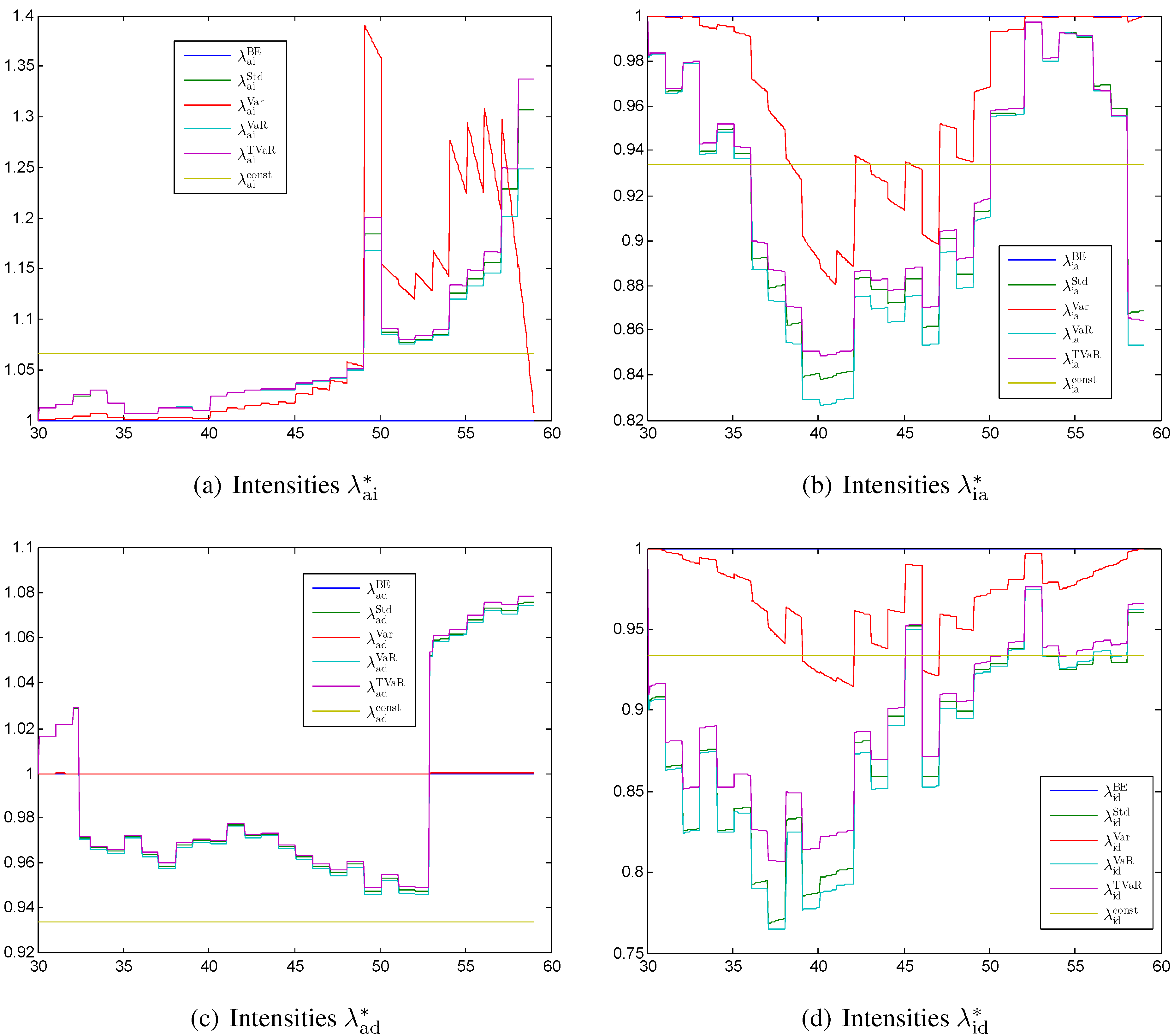
In Figure 2 the first order intensities ${\lambda }_{\mathrm{ai}}^{*}$, ${\lambda }_{\mathrm{ia}}^{*}$, ${\lambda }_{\mathrm{ad}}^{*}$, and ${\lambda }_{\mathrm{id}}^{*}$ calculated with different principles are shown as percentages of ${\lambda }^{BE}$. The stochastic model used in this section is time-discrete so that the intensities are constant within one year. This is the reason why most of the intensities of first order are also mostly constant within one year. The intensities calculated with the variance principle are an exception; they are strongly influenced by the sum at risk and thus alternate more.

In Figure 2a we see that the intensities ${\lambda }_{\mathrm{ai}}^{*}$ have the highest safety margin and strongly increase at the end of the contract. Only the intensity calculated with the variance principle is going back to the best estimate case, since the sum at risk is zero at the end of the contract. The high value around age 50 is due to an outlier that transferred to ${\varphi }_{\mathrm{ai}}\left(x\right)$. The standard deviation, the value at risk, and the tail value at risk principles all lead to comparable results. The constant level is at the beginning larger than the other methods and at the end significantly smaller.

Figure 2. First order intensities ${\lambda }^{*}$ for (a) the transition $(\mathrm{a},\mathrm{i})$; (b) the transition $(\mathrm{i},\mathrm{a})$; (c) the transition $(\mathrm{a},\mathrm{d})$; (d) the transition $(\mathrm{i},\mathrm{d})$ each calculated with different principles (values given relative to ${\lambda }^{BE}$).

Figure 2. First order intensities ${\lambda }^{*}$ for (a) the transition $(\mathrm{a},\mathrm{i})$; (b) the transition $(\mathrm{i},\mathrm{a})$; (c) the transition $(\mathrm{a},\mathrm{d})$; (d) the transition $(\mathrm{i},\mathrm{d})$ each calculated with different principles (values given relative to ${\lambda }^{BE}$).

The intensities ${\lambda }_{\mathrm{ia}}^{*}$ in Figure 2b have a negative safety margin. Since the deterministic function ${\varphi }_{\mathrm{ia}}$ is close to zero between age 50 and 55, the corresponding transition rate is almost deterministic. Consequently, the intensities are returning to the best estimate level between age 50 and 55 with most of the principles.

The intensity ${\lambda }_{\mathrm{ad}}^{*}$ shown in Figure 2c has the lowest safety margin. The safety margin has two sign changes. The first one after a few years and the second one between age 53 and 54. The first sign change is due to the fact that the best estimate reserve $V_{\mathrm{a}}^{BE}\left(0\right)$ is negative at the beginning of the contract. This is the case since we calculated the premium such that $V_{\mathrm{a}}^{*}\left(0\right)=0$. At the end of the contract we have again a sign change, since the reserve of an active policyholder is negative for the last years of the contract. The variance principle suggests only a tiny margin, since the sum at risk for the transition from active to dead is small compared with other sums at risk.

We would expect that the intensities ${\lambda }_{\mathrm{id}}^{*}$ shown in Figure 2d are decreasing monotonically. However, the first order intensities ${\lambda }_{\mathrm{id}}^{*}$ are going back to the best estimate case at the end of the contract. This is due to the stochastic model for the intensity ${\lambda }_{\mathrm{id}}$, where ${\varphi }_{\mathrm{id}}\left(x\right)$ is mainly decreasing from 1 to 0 during the time of the contract and consequently there is less uncertainty at the end of the contract. Furthermore, the values of ${\varphi }_{\mathrm{id}}\left(x\right)$ alternate so that the resulting intensities ${\lambda }_{\mathrm{id}}^{*}$ alternate over time as well.

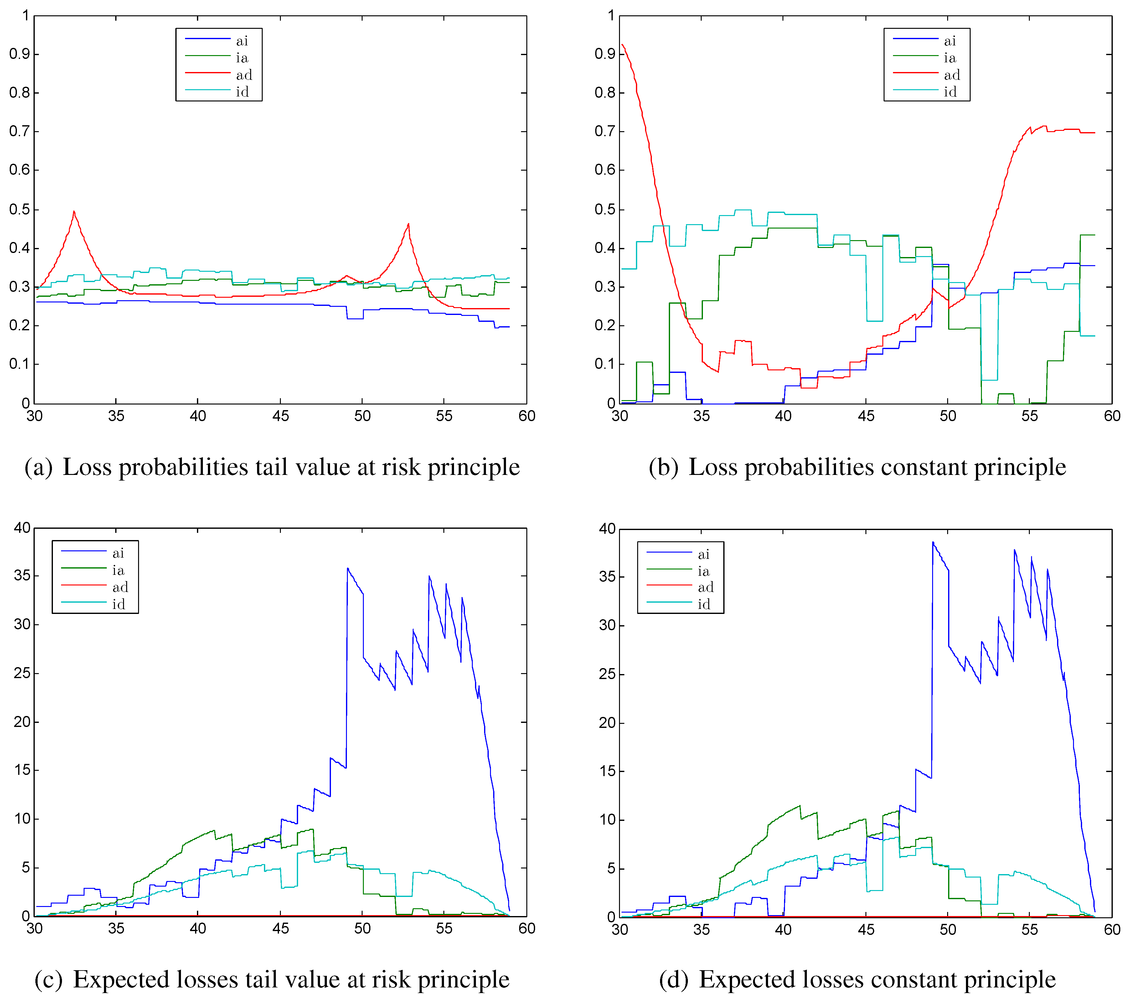
Figure 3. Loss probabilities calculated with (a) the tail value at risk principle; (b) the constant principle; expected losses calculated with (c) the tail value at risk principle; (d) the constant principle.

Figure 3. Loss probabilities calculated with (a) the tail value at risk principle; (b) the constant principle; expected losses calculated with (c) the tail value at risk principle; (d) the constant principle.

4.1.2. Loss Probabilities and Expected Losses

In Figure 3 we see the corresponding loss probabilities and expected losses calculated with the tail value at risk principle and the constant principle. We choose exemplarily the tail value at risk principle, since the results with the standard deviation principle and the value at risk principle are similar. The loss probabilities calculated with the tail value at risk principle in Figure 3a are quite constant compared with the loss probabilities calculated with the constant principle shown in Figure 3b. While the sign changes in the reserve of an active policyholder only lead to two peaks in the loss probability for the transition from active to dead in Figure 3a, the loss probability calculated with the constant principle is at the beginning of the contract close to 1 and increases at the end of the contract again to close to $70\%$, since the constant principle cannot reproduce the sign change. The peak at age 50 in Figure 2a for the transition $(\mathrm{a},\mathrm{i})$ even leads to a trough in the loss probability at age 50 for the tail value at risk principle. In contrast, it leads to a peak in the loss probabilities calculated with the constant principle.

However, the expected loss has a peak at age 50 for both the tail value at risk principle and the constant principle, as we can see in Figure 3c,d. The expected losses look very similar for the two principles with the only difference that the level of the constant principle is a little bit higher. However, the absolute amounts of the expected losses are at most 35, which is quite moderate compared with the premium of around 300 and the annuity of $10,000$. The expected losses are dominated by the transition from active to invalid in the second half of the contract. This justifies the high safety margins that we saw in the second half of Figure 2a for the standard deviation, value at risk, and tail value at risk principles. The loss probabilities are slightly decreasing with the tail value at risk principle so that the high expected losses can be compensated a little bit. With the constant principle, the loss probabilities for the transition $(\mathrm{a},\mathrm{i})$ are nearly twice as high as for the tail value at risk principle, thus the high expected loss leads to a high risk for the insurance company when using the constant principle.

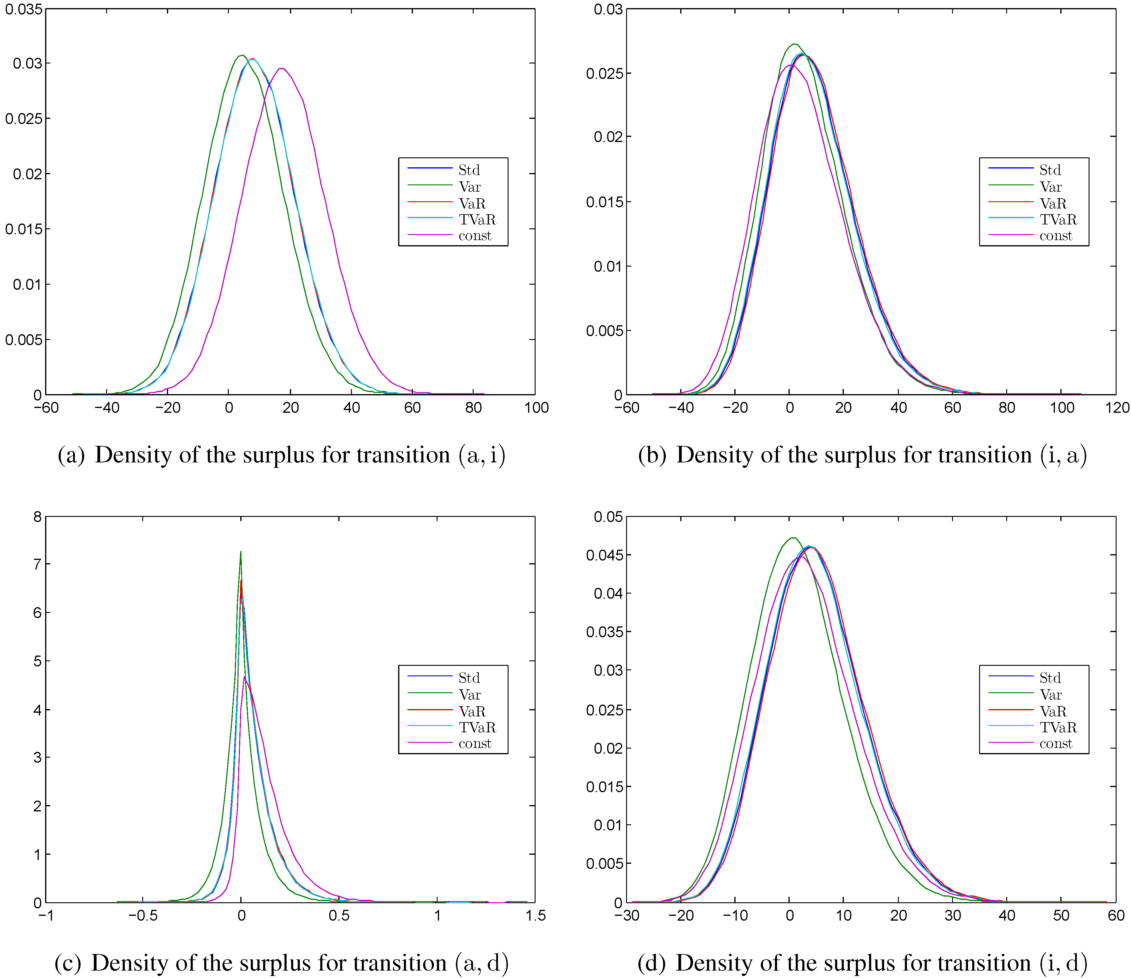
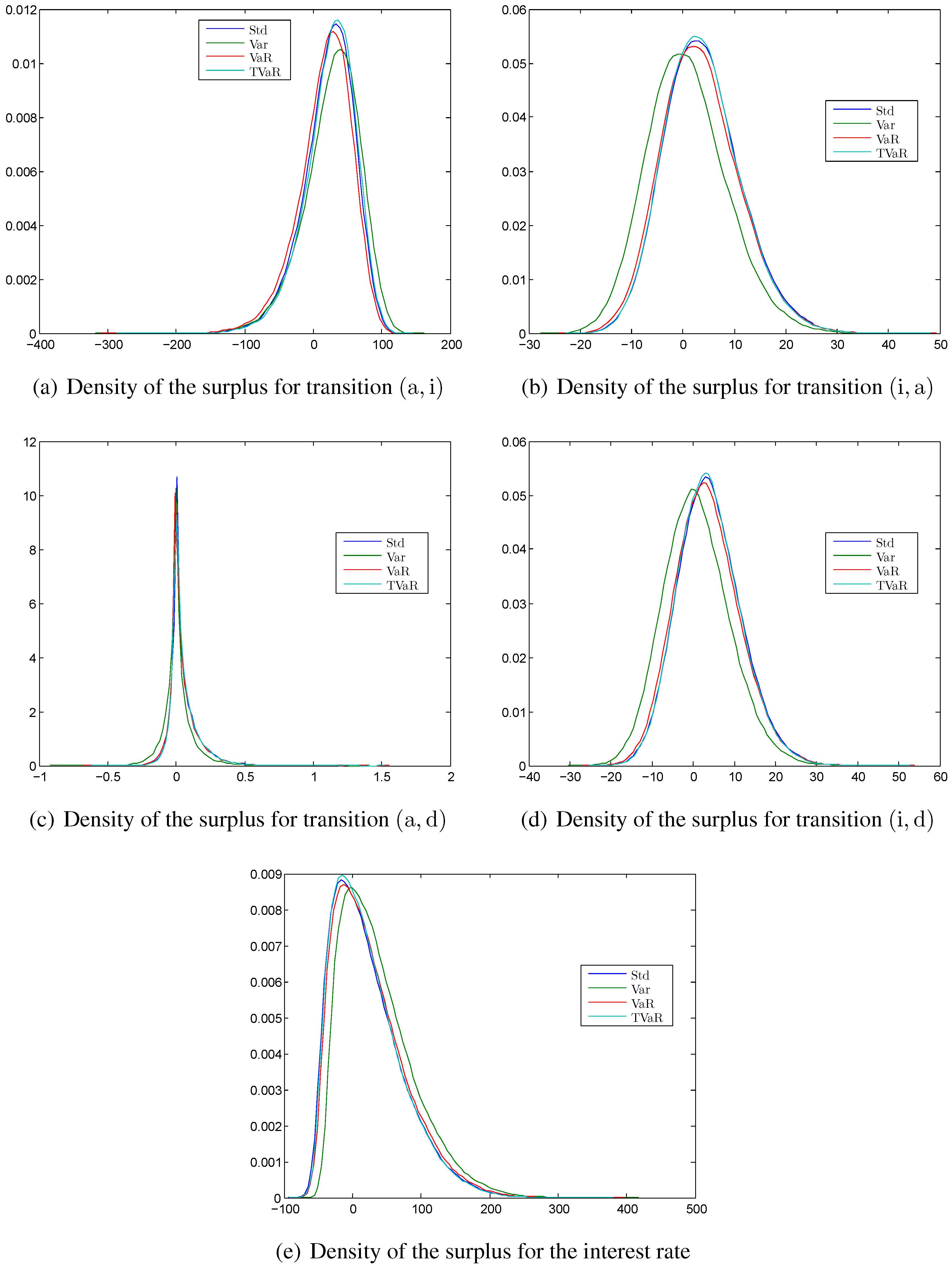
Figure 4. Kernel density estimation of the surplus at time $t=15$ for different principles calculated with the MATLAB function ksdensity for (a) the transition $(\mathrm{a},\mathrm{i})$; (b) the transition $(\mathrm{i},\mathrm{a})$; (c) the transition $(\mathrm{a},\mathrm{d})$; (d) the transition $(\mathrm{i},\mathrm{d})$.

Figure 4. Kernel density estimation of the surplus at time $t=15$ for different principles calculated with the MATLAB function ksdensity for (a) the transition $(\mathrm{a},\mathrm{i})$; (b) the transition $(\mathrm{i},\mathrm{a})$; (c) the transition $(\mathrm{a},\mathrm{d})$; (d) the transition $(\mathrm{i},\mathrm{d})$.

As a result, we see that it is indeed possible with the proposed allocation method to smooth the loss probabilities considerably. This underlines the adequacy of the method. However, the expected losses are not significantly improved.

4.1.3. Empirical Densities of the Surplus

In Figure 4 the densities of an instantaneous loss at time 15 are shown for all four transitions , i.e., the probabilities that the integrands of Equation (2) are negative. We see that using different safety margins does not change the shape of the density but merely shift them to the left or right. This is because a safety margin is just one deterministic value that does not affect the probability distribution of the random transition rates. In general, the densities are mostly symmetric and the different safety margins lead to a shift of the densities. The consequence is that the standard deviation, the value at risk, and tail value at risk principles lead to similar results. The surplus (and so the losses) are significantly smaller for the transition $(\mathrm{a},\mathrm{d})$. As mentioned before this is the case since the reserve for an active policyholder is significantly smaller than for an invalid policyholder.

4.2. Case (b): Disability Insurance with Interest Rate Risk

Now we add interest rate risk to the model from case (a). Therefore, we model the interest rate stochastically with the model from Cox, Ingersoll, and Ross (CIR) proposed in [17]. The short rate follows the differential equation

$$\begin{array}{c}\hfill \mathrm{d}r\left(t\right)=\kappa (\theta -r\left(t\right))\mathrm{d}t+\sigma \sqrt{r\left(t\right)}\mathrm{d}{W}_t,\end{array}$$

which is approximated by the Euler–Maruyama method as above. We adopt the calibration of the model from [18] with the difference that we set the short rate at time zero to the currently more accurate value of $r\left(0\right)=0.02$. The values are summarized in Table 3.

Table 3. Parameters of the CIR process (cf. [18]).

Variable	Value	Description
$r\left(0\right)$	$0.02$	starting value
κ	$0.2$	mean reversion speed
θ	$0.04$	mean reversion level
σ	$0.1$	volatility of the model

Table 3. Parameters of the CIR process (cf. [18]).

Variable	Value	Description
$r\left(0\right)$	$0.02$	starting value
κ	$0.2$	mean reversion speed
θ	$0.04$	mean reversion level
σ	$0.1$	volatility of the model

Since the Feller condition $2\kappa \theta \ge {\sigma }^2$ is fulfilled, the process ${\left(r\left(t\right)\right)}_{t\ge 0}$ is theoretically always strictly positive. The model for the transition rates, the contract specifications, and all other parameters are the same as in case (a). In this example, we get a premium of $B_{\mathrm{a}}\left(\tau \right)=-301.18\tau$ compared with $B_{\mathrm{a}}\left(\tau \right)=-312.02\tau$ in case (a).

4.2.1. First Order Transition and Interest Rates

The calculated first order intensities, as well as the first order short rate, the loss probabilities, the expected losses and the density functions, are shown in Figure 5 and Figure 6. For this model we do not calculate the intensities with the constant principle, since it is unclear how we should compare the interest rate with the intensities. It does not seem to be appropriate to take the same factor, since the volatility in the short rate model is much higher. In contrast, the method proposed in Section 3 enables us to calculate the first order transition intensities and short rate within one framework.

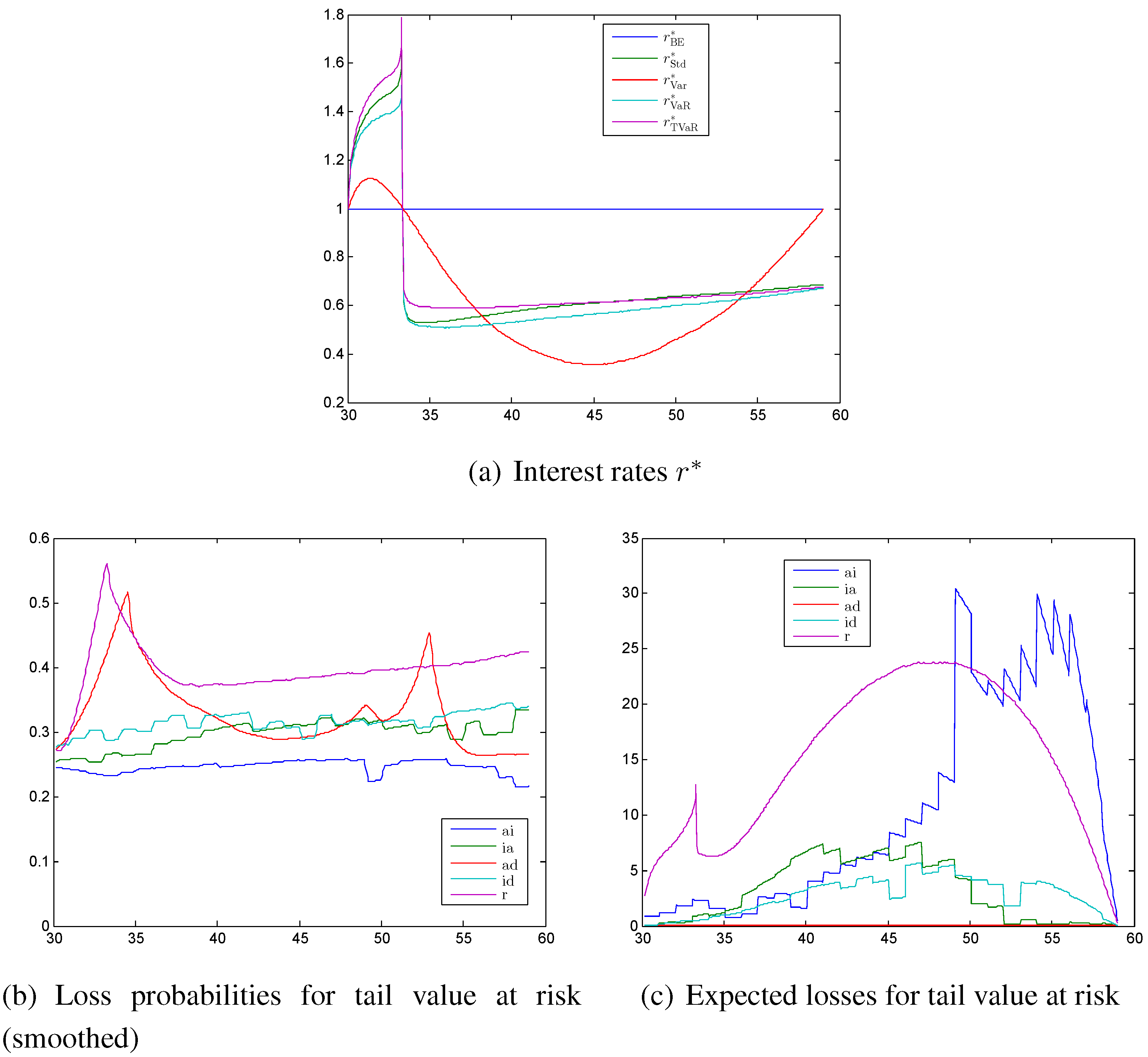
Figure 5. (a) First order interest rates $r^{*}$ calculated with different principles (values given relative to $r^{BE}$; (b) loss probabilities; and (c) expected losses each calculated with the tail value at risk principle.

Figure 5. (a) First order interest rates $r^{*}$ calculated with different principles (values given relative to $r^{BE}$; (b) loss probabilities; and (c) expected losses each calculated with the tail value at risk principle.

The first order interest rate is shown in Figure 5a. It is first increasing and then we have a rapid sign change after around 3 years. This is the point where ${\sum }_{j\in S}{V}_j^{BE}(\tau -)p_{\mathrm{a}j}^{*}(0,\tau )$ changes its sign from negative to positive. Consequently, we have an asymptote and have to be careful with the numerics. With the standard deviation, the value at risk, and the tail value at risk principles, the first order interest rate has a level of $50\%$ to $60\%$ of the best estimate value after 4 years and is then slowly increasing to a level between $60\%$ to $70\%$. We see here minor differences between the three principles. In particular, the interest rate calculated with the tail value at risk principle has at the beginning a higher level than the others and then increases only very slowly in time. The level of about $60\%$ matches the German law where in §65 Versicherungsaufsichtsgesetz it is required that the technical interest rate is smaller than $60\%$ of the interest rate of government bonds. Thus it seems as if our result confirms the suitability of this law. At the end of this section, we will make a sensitivity analysis of this level with respect to the parameters of the interest rate model. The first order interest rate calculated with the variance principle has for most of the time a very large safety margin, but increases at the end to the best estimate case, since the reserve of an active and an invalid policyholder is going to zero at the end of the contract. In contrast to other principles, the weighted reserves do not cancel in Equation (7). We do not show the safety margins for the transitions intensities again, since they are basically equal to the ones from case (a). The only exception is that the intensities calculated with the variance principle have a significant lower level when adding interest rate risk.

4.2.2. Loss Probabilities and Expected Losses

The probabilities of having a loss are shown in Figure 5b for the tail value at risk principle. We smoothed them with the moving average method with a span of $n/4$, in particular to avoid the oscillation in the loss probability of the interest rate risk resulting from the Monte Carlo simulations. The loss probabilities for the transition rates are similar to those from Figure 3a, only except that the level is slightly lower and therefore the probabilities are slightly increasing in time. The loss probability for the interest rate is at the beginning of the contract increasing considerably and then only slightly. The general level is higher than for the intensities. After around 3 years we have a peak resulting from the sign change of the weighted reserves.

The corresponding expected losses shown in Figure 5c are again similar to the intensities from case (a). The expected loss coming from the interest rate is monotonically increasing until age 48 with exception of the peak after 3 years. After that the probability decreases to zero again. These two figures might lead to the conclusion that the interest rate risk dominates the biometric risk. We have to keep in mind that we implicitly assume that our artificial insurance company invests all its money in the short rate or a corresponding bank account. This is far away from reality, since life insurance companies usually invest their money in bonds with long maturities and therefore do not face such a huge interest rate risk. The modeling of the assets of an insurance company is very complex, which we avoided here. With a “correct” model for the assets we would have to make a lot of assumptions and we also would no longer see which effects are coming from the asset model and which are general effects.

In general we have similar results as in Section 4.1. The loss probabilities are quite constant while the expected losses are significantly increasing or decreasing.

Figure 6. Kernel density estimation of the surplus at time $t=20$ for different principles calculated with the MATLAB function ksdensity for (a) the transition $(\mathrm{a},\mathrm{i})$; (b) the transition $(\mathrm{i},\mathrm{a})$; (c) the transition $(\mathrm{a},\mathrm{d})$; (d) the transition $(\mathrm{i},\mathrm{d})$; and (e) the interest rate.

Figure 6. Kernel density estimation of the surplus at time $t=20$ for different principles calculated with the MATLAB function ksdensity for (a) the transition $(\mathrm{a},\mathrm{i})$; (b) the transition $(\mathrm{i},\mathrm{a})$; (c) the transition $(\mathrm{a},\mathrm{d})$; (d) the transition $(\mathrm{i},\mathrm{d})$; and (e) the interest rate.

4.2.3. Empirical Densities of the Surplus

The density functions of the transition rates and the interest rate in Figure 6 at time $t=20$ are no longer symmetric but skewed instead. In particular, Figure 6a shows that the intensity for the transition $(\mathrm{a},\mathrm{i})$ has a heavy tail on the loss side. This is the case since ${\lambda }_{\mathrm{ai}}^{BE}$ is hardly over $1\%$ during the time of the contract. The intensity is bounded by zero but can be significantly positive. This results in the skewed density function with the heavy tail on the loss side. In contrast, the densities in Figure 6b–e have a heavy tail on the profit side, which is of course not a big issue from a risk manager’s perspective. They all include a negative safety margin meaning that the high intensities indicate a gain and the loss is bounded, since the intensities cannot be smaller than zero. Consequently, we also see more differences between the risk measures standard deviation, value at risk, and tail value at risk. The skewed functions also explain why we show in this section the loss probabilities and the expected loss for the tail value at risk principle. These density functions seem to require a risk measure that takes into account the tails on the loss side as the tail value at risk does. Consequently, we see in Figure 6a that the density function calculated with the tail value at risk principle is shifted the most to the right (to the profit side). The density function of the interest rate in Figure 6e is more skewed than the others, since the interest rate has a high probability to be close to zero, whereas the intensities have a lower probability to be close to zero. Comparing the x-axes of the different densities, we see that the transition $(\mathrm{a},\mathrm{i})$ and the interest risk dominate all other risk sources. Since the transition from active to invalid has a heavy tail with losses that exceed the yearly premium, this transition seems to imply more risk than the interest rate. With the interest rate risk we have a high probability to obtain a loss close to 100, but there are hardly any larger losses. To conclude, the proposed method with the tail value at risk takes into account the risky tails, but can—as it holds for any other safety margin—only shift the density function and cannot change the tail.

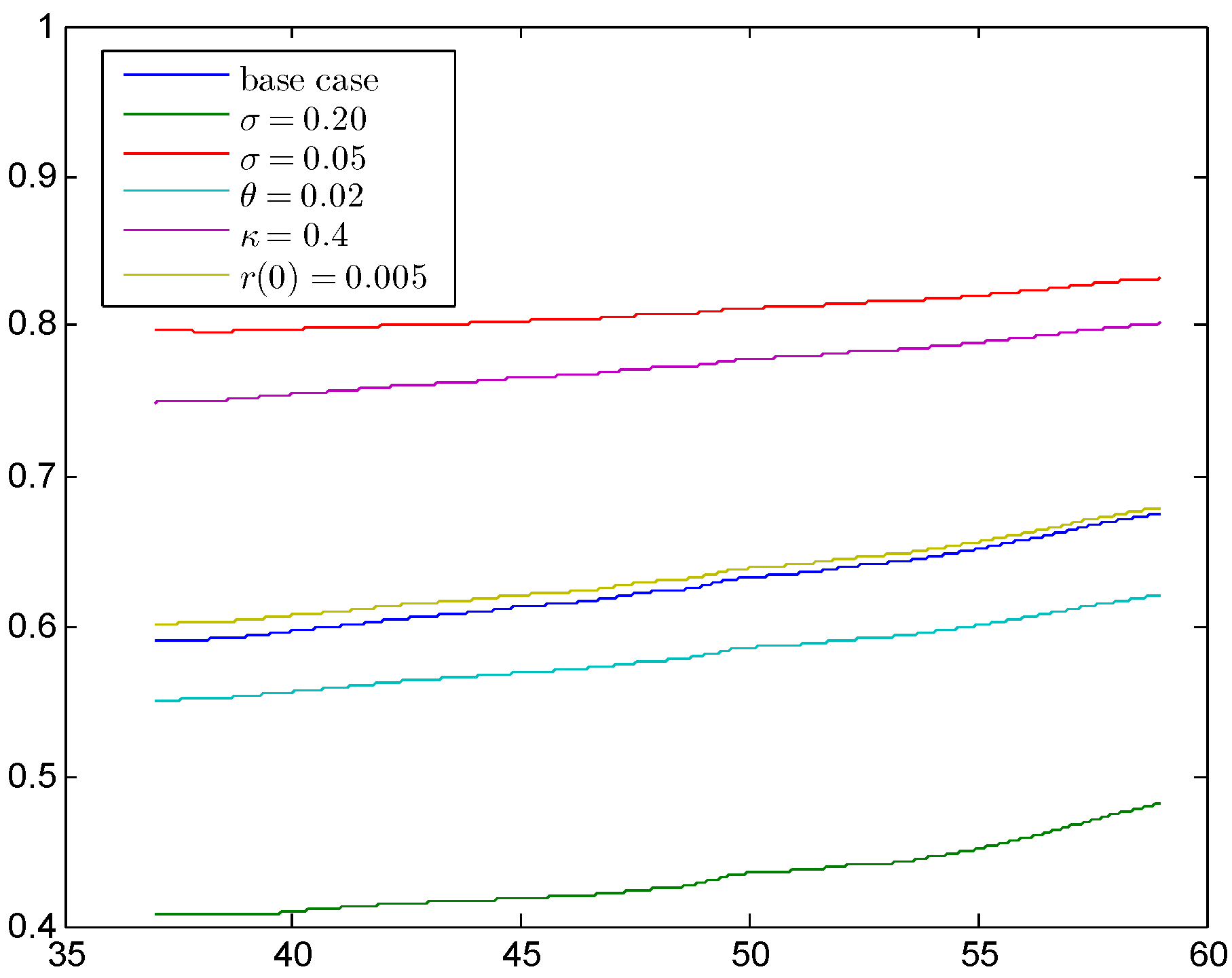
4.2.4. Sensitivity Analysis of the First Order Interest Rate

In Figure 5a we have seen that our model requires a first order interest rate of about $60\%$ of the best estimate interest rate, which corresponds to the German regulation praxis. In what follows, we want to investigate how reliable this result is. Therefore, we calculate five sensitivities of the model from above with the tail value at risk principle by taking different parameters for the short rate model. The results are shown in Figure 7 together with the above case as base case.

Figure 7. Sensitivities for the first order interest rate calculated with the TVaR (smoothed).

Figure 7. Sensitivities for the first order interest rate calculated with the TVaR (smoothed).

To focus on the main parts, we have smoothed the results again by the moving average method with a span of n and we also show the results starting with age 37, since the peak before is not relevant for the main level. First of all, we have changed the volatility σ to $0.20$ and $0.05$, respectively, which is a large change compared with the initial level of $0.1$. We see that the short rate level fundamentally changes; more precisely, we get a level of $40\%$ to $50\%$ and of around $80\%$, respectively. Reducing the mean reversion level θ from $0.04$ to $0.02$ reduces the main level by $5\%$, which is quite small compared with the volatility change. Increasing the mean reversion speed κ from $0.2$ to $0.4$ results in a significant increase to $75\%$ to $80\%$. Changing the initial interest rate from $r\left(0\right)=0.02$ to $r\left(0\right)=0.005$ does not change the main level significantly. In total, this analysis shows that the percentage of the first order interest rate with respect to the best estimate interest rate is not fixed at around $60\%$, but changes considerably with the parameters of the short rate model. Furthermore, this level also changes with the safety level α, which is not shown here.

5. Semi-Markov Invalid-Dead Model

In this section, we demonstrate how the safety margins look like in a semi-Markov model. Therefore, we pick up the so-called Danish model ([19], pp. 100–102), which is a model for a disability insurance as in Figure 1, but with the difference that reactivation of a disabled person is not possible. We model the mortality rate of the disabled policyholder by the semi-Markov model presented in [20]. The transition intensities from active to invalid and from active to dead are given by (cf. [19], p. 100)

$$\begin{array}{c}\hfill {\lambda }_{\mathrm{ai}}\left(x\right)=0.0004+{10}^{0.06x-5.46}\text{and}{\lambda }_{\mathrm{ad}}\left(x\right)=0.0005+{10}^{0.038x-4.12},\end{array}$$

(13)

where x is the age of the policyholder. Consequently, we assume that these two transition rates are deterministic. In [19] it is assumed that ${\lambda }_{\mathrm{id}}\left(x\right)={\lambda }_{\mathrm{ad}}\left(x\right)$, which we do not adopt. However, we assume that the transition rates ${\lambda }_{\mathrm{id}}$ depend on the time spent in the state invalid and that they are time-dependent. Only the future transition rates from invalid to dead are random, so we only need safety margins for this transition. From the last section we know that this transition is not the one with the most risk for an insurance company and it could be more seen as a toy example to demonstrate the method within a semi-Markov model. Note that we cannot consider just an invalid-dead model, since the policyholder would then have one duration at inception of the contract and this would hold for every point in time. In contrast, in the specified model the point in time when the policyholder gets invalid is random. The transition intensities from invalid to dead are considered to fulfill the following model (compare [20])

$$\begin{array}{c}\hfill log\left({\lambda }_{\mathrm{id}}(x,d,t)\right)={\alpha }_x{\gamma }_d+{\beta }_x{\kappa }_t\text{for}x,d,t\in \mathbb{N},\end{array}$$

where ${\lambda }_{\mathrm{id}}(x,d,t)={\lambda }_{\mathrm{id}}(\left[x\right],\left[d\right],\left[t\right])$ and x is the age, d the duration in the state invalid, and t the time. We adopt the calibration of the model from [20], where $x\in \{40,...,59\}$ and $d\in \{0,...,6\}$ and we assume that $d=6$ is representative for all durations larger than 6. The model is fitted to data from the German statutory pension insurance (Deutsche Rentenversicherung) from the years 1994 to 2009 and we adopt the calibration of the ARIMA(0,1,0) model for the time parameter ${\kappa }_t$ to forecast the model into the future.

The parameters of the example are shown in Table 4. In this section we use a semi-Markov model, so the Euler–Maruyama method has to be applied in time and duration, which makes the numerical calculations more expensive. Therefore, we have to reduce the number of Monte Carlo simulations. Nevertheless, the results are still robust as we verify in further analyses. An explanation is that there is no interaction between different rates, which makes the results more stable.

Table 4. Parameters for the semi-Markov model.

Variable	Value	Description
N	$10,000$	number of Monte Carlo simulations
n	10	number of steps per year for the Euler–Maruyama method
α	$0.95$	safety level in Equation (3)
β	$0.80$	safety level for the risk measures value at risk and tail value at risk
$B_{\mathrm{i}}\left(\tau \right)$	$10,000\tau$	payment function for the annuity payment in state invalid
$x_0$	40	initial age of the insured
T	15	duration of the contract

Table 4. Parameters for the semi-Markov model.

Variable	Value	Description
N	$10,000$	number of Monte Carlo simulations
n	10	number of steps per year for the Euler–Maruyama method
α	$0.95$	safety level in Equation (3)
β	$0.80$	safety level for the risk measures value at risk and tail value at risk
$B_{\mathrm{i}}\left(\tau \right)$	$10,000\tau$	payment function for the annuity payment in state invalid
$x_0$	40	initial age of the insured
T	15	duration of the contract

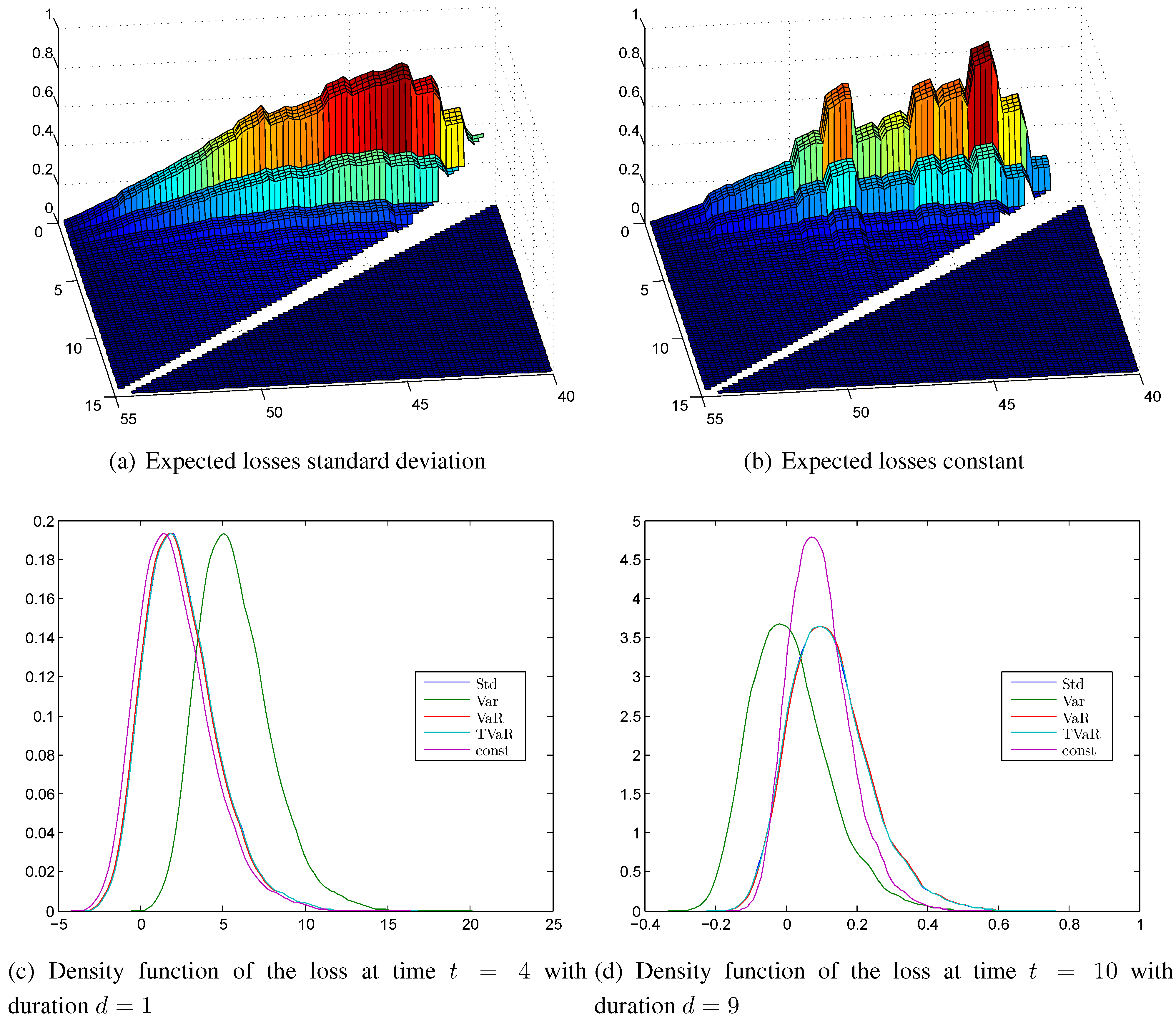
Figure 8. First order intensities ${\lambda }_{\mathrm{id}}^{*}$ calculated with (a) the standard deviation principle; (b) the variance principle (values given in relation to ${\lambda }_{\mathrm{id}}^{BE}$); loss probabilities calculated with (c) the standard deviation principle; (d) the constant principle.

Figure 8. First order intensities ${\lambda }_{\mathrm{id}}^{*}$ calculated with (a) the standard deviation principle; (b) the variance principle (values given in relation to ${\lambda }_{\mathrm{id}}^{BE}$); loss probabilities calculated with (c) the standard deviation principle; (d) the constant principle.

Since ${\lambda }_{\mathrm{ai}}$ and ${\lambda }_{\mathrm{ad}}$ are deterministic, the payment function in the state active is not relevant for the calculation of the safety margins of the transition rates. The resulting transition rates and the probabilities of having a loss are shown in Figure 8 and the expected losses and selected density functions are shown in Figure 9. Since we consider now a semi-Markov framework, the first order transition rates ${\lambda }_{\mathrm{id}}^{*}$ are two-dimensional. In what follows, we investigate the appropriateness of our method in such a framework.

Figure 9. Expected losses calculated with (a) the standard deviation principle; (b) the constant principle; kernel density estimation of the surplus (c) at time $t=4$ (duration $d=1$); (d) at time $t=10$ (duration $d=9$).

Figure 9. Expected losses calculated with (a) the standard deviation principle; (b) the constant principle; kernel density estimation of the surplus (c) at time $t=4$ (duration $d=1$); (d) at time $t=10$ (duration $d=9$).

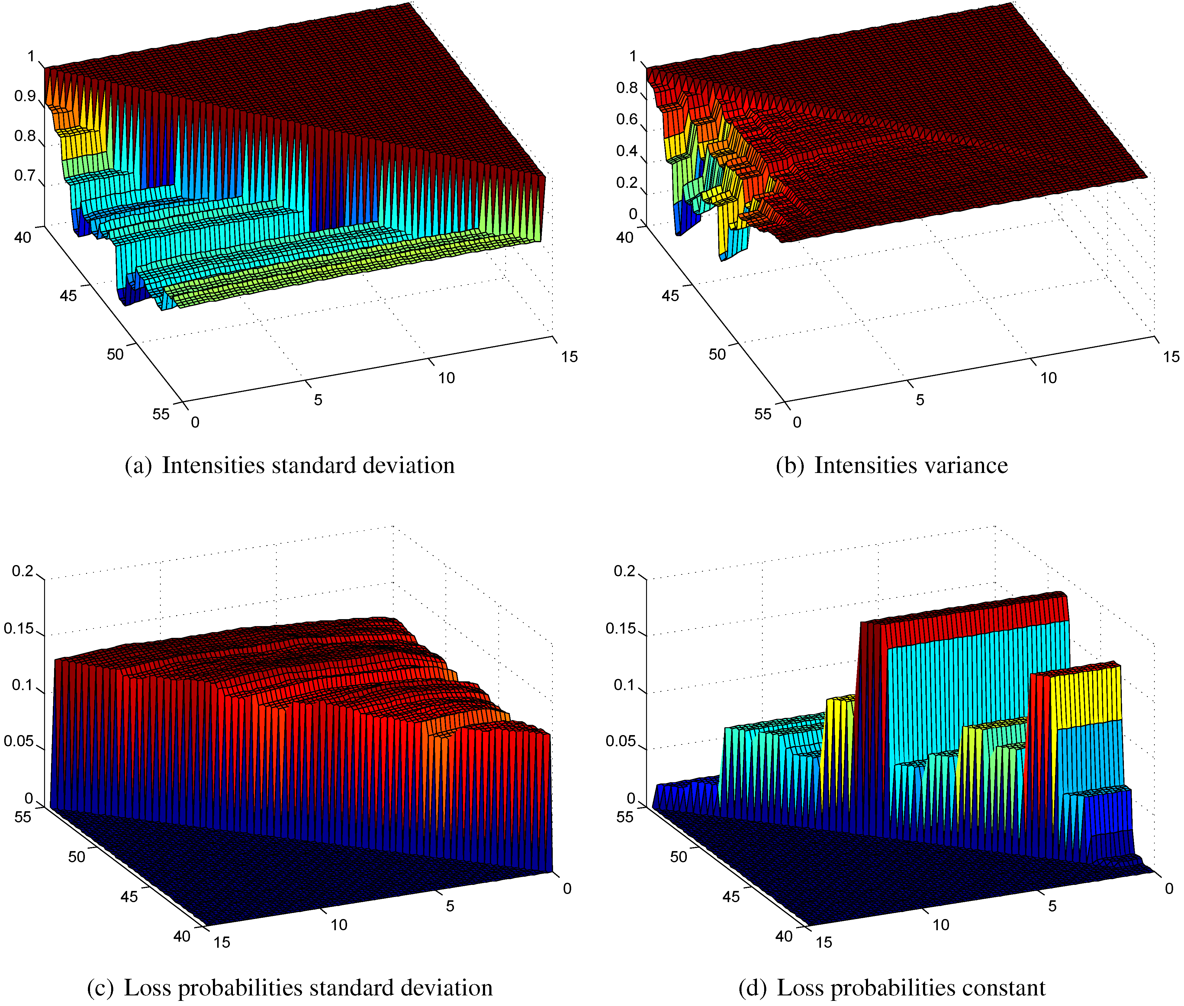
5.1. First Order Transition Rates

In Figure 8a,b we see the first order intensities ${\lambda }_{\mathrm{id}}^{*}$ calculated with the standard deviation and the variance principles. We do not show the intensities calculated with the value at risk and the tail value at risk principles, since they are nearly equal to the one calculated with the standard deviation principle. The constant principle results in a first order intensity with a constant level of $73.6\%$ of the best estimate intensity. The intensities calculated with the standard deviation principle show steps for the different ages and are quite constant with respect to the duration. This can be explained by the model in Equation (13), where all the randomness is modeled by ${\kappa }_t$, which only affects the age parameter ${\beta }_x$. Consequently, there is no randomness in the duration, so the proportion to the best estimate intensity is quite constant. This is not the case for the variance principle, since the sum at risk plays a crucial role here and the safety margin calculated with the variance principle is zero at the end. In contrast, the safety margin is very high at the beginning of the contract. However, the scale of the z-axis shows that the resulting safety margin calculated with the variance principle is quite extreme. For these reasons, we do not study the variance principle anymore and focus on the other three principles. Since they are very similar, we study basically only the standard deviation principle and compare it with the constant principle.

5.2. Loss Probabilities and Expected Losses

Figure 8c shows the loss probabilities for the intensities calculated with the standard deviation principle. They are more or less constant in time and in duration. Therefore, our proposed allocation method for calculating safety margins produces also good results in a duration-dependent framework. The loss probabilities of the constant principle shown in Figure 8d are quite constant in duration but significantly different in age. The corresponding expected losses in Figure 9a,b are similar; the ones of the standard deviation principle are smoother compared with the constant principle, but the level is comparable.

5.3. Empirical Densities of the Surplus

The density functions are shown for time $t=4$ and duration $u=1$ in Figure 9c and time $t=10$ and duration $u=9$ in Figure 9d. They are both roughly symmetric with a slight tail on the profit side. We see that the standard deviation, the value at risk, and the tail value at risk principles are not distinguishable. At time $t=4$ with the low duration the constant principle has a lower safety margin, and at time $t=10$ the safety margins of the constant principle and the standard deviation principle are similar. The absolute values of the expected losses and of the x-axes of the densities are quite low, compared with the disability annuity of $10,000$ and also compared with the results of Section 4.

All in all, the standard deviation principle, the value at risk, and the tail value at risk principles perform well with this semi-Markov model, whereas the variance principle does not seem to be favorable. The constant principle leads to loss probabilities that are jumping with different ages, which does not seem to be adequate for an insurance company.

6. Conclusions

The paper proposes a risk-oriented method for the allocation of the total safety margin to different points in time and transitions. The formulas are presented within a very general semi-Markov framework and allow the use of different risk measures. In a case study, we apply the method to two different life insurance contracts and deduce safety margins for them. The results are very promising, since the calculated transition rates of first order lead to quite constant ruin probabilities, whereas they significantly vary over time with the classical time-constant method. The latter is calculated as a constant percentage of the best estimate calculation basis. Our results show that the technical interest rate should be equal to around $60\%$ of the best estimate. However, this value heavily depends on the parametrization of the interest rate model, as we show in a sensitivity analysis.

A weakness of our method is that for the calculation of the safety margins we decompose $V^{*}(t,u)-V^{BE}(t,u)$ and $-(V(t,u)-V^{BE}(t,u))$, whereas for the surplus we consider the decomposition of $V^{*}(t,u)-V(t,u)$. These two decompositions are different and we would obtain even better results should we also use the first one to define the surplus, but we followed the standard practice in the literature that uses only the latter. It should be kept in mind that there are no mathematically established arguments for one or the other decomposition. Another drawback of our proposed method is that we need a safety margin for every contract.

For the calculation of the safety margin, stochastic models are needed that describe the future development of the calculation basis. In spite of the rich literature on models for mortality rates, there are only a few models for multi-state insurance products. More research is needed here in order to make the method more applicable.