1. Introduction
Defined benefit (DB) and defined contribution (DC) plans are two important types of private retirement plans in developed countries. In a DB plan, the employee’s pension benefit is determined by a formula, which takes into account years of service for the employer and wages or salary. In a DC plan, sponsoring companies (and often, also, their employees) pay a promised contribution to an external pension fund, which invests the contributions in financial assets. The pension payment is then simply determined as the market value of the backing assets. The DB plan was the dominant form of plan, but in the last decade, the number of DC plans has a steady upward-moving trend. For instance, according to the U.S. Flow of Funds Accounts, the division between assets held in private DB plans and private DC plans was 60% versus 40% in 1987, and in 2007, this division was reversed. In the U.K., the Government Actuary’s Department observed that final salary DB plans constituted 92% of all pension funds in 1979, and this number was reduced to 41% in 2005.
There are quite some significant tradeoffs between DB and DC plans, particularly when it comes to what risks the employees bear. [
1,
2] provide a very extensive review on the tradeoffs. In this place, we want to emphasize three tradeoffs with respect to investment, portability and salary risk. In a DB plan, the sponsoring company is responsible for providing promised (future) pension benefits to the employees. In other words, the sponsoring company decides about investment policies in a pension fund and, consequently, also bears the entire investment risks in a DB plan. In a DC plan, the company does not ensure a promised pension payment to the employees. The employees bear the entire investment risks. From the employees’ perspective, salary risk is present in both the DB plan and the DC plan. In the former plan, the employee bears the salary risk, because the defined benefits are usually directly linked to his salary, while in the latter plan, the amount of contributions the employee can make mainly depends on the development of his salary. Portability risk is the risk not to have the ability to transfer years of credited service or accumulated benefits from one employer to another. It is widely accepted knowledge that portability risk plays a minor role in DC plans, while it is considered as the driving source of risk in single employer DB pension plans. Since the pension payment of a DC plan mainly depends on the value of the backing assets, a DC plan can be easily ported between job switching. On the contrary, DB plan holders lose mostly part of their benefits after changing jobs, since most DB plans lack portability provisions.
In a DC plan, the asset price risk is the most important risk factor, since the accumulated pension benefit of the employee is the market value of the contributions made while working and the investment returns earned on the plan balances. [
3,
4] measure risk in the DC plan by computing VaR estimates during the accumulation phase. They find that the asset allocation strategy mainly drives the asset price risk, since the VaR estimates are considerably more sensitive to the asset allocation strategy than to the choice of the asset return model.
Portability risk is considered the main risk factor in DB plans, especially because of the huge and increasing workforce mobility and the fact that only a few single employer DB programs contain portability provisions
1. [
5] reports that workers in the U.S. hold 10 or 11 jobs during their working lives. [
1] mentions that fewer than 5% of workers remain with the same employer and that the average worker in the U.K. changes jobs about six times in a life time. [
6] further points out that job turnover increased substantially in the 1990’s compared to earlier decades. [
8] provides a detailed analysis of portability risk. In particular, they quantify different types of portability losses, like the cash equivalent loss and back-loading loss for different deterministic wage paths and the number of job moves in the U.K. Specifically, they report that even a low number of job moves can cause huge portability losses, for instance someone changing jobs once mid-career can lose up to 16% of the full service pension. A typical U.K. worker moving six times in a career could end up with a pension of only 70%–75% of the pension of a worker with the same salary experience who remains in the same job for his whole career.
Our main contribution to the literature about the comparison of DB and DC pension plans is that we provide a formal model for comparing the two major types of private retirement plans by explicitly taking account of their most important risk factors: stochastic wages, job moving and asset prices. We compare the DB with the DC plan in an expected utility-based framework. In the utility-based analysis of the occupational pension plans, there are mainly two streams of literature. The first stream tries to solve the utility maximization problem and/or the optimal investment strategy for the occupational plans. In the second stream, utility-based comparisons are made among several given contracts. Contract A is better than Contract B, if it delivers a higher expected utility. In this sense, it does not contain a utility maximization problem. Our paper belongs to the latter case. We aim to model realistic properties of the two plans and make reasonable comparisons between them. Three frequently-used utility functions in the pension insurance literature are considered: power utility, mean-shortfall and mean-downside deviation. The latter two utility functions penalize the realizations of the terminal pension payment below a threshold, demonstrating the loss-aversion property. Under mean-shortfall, the penalty has a linear form. Mean-downside deviation punishes the loss more severely, and the loss takes a quadratic form. We mainly examine under what parameter combinations the beneficiary is indifferent between the DB and DC plan.
Our methodology to compare the two pension retirement plans is similar to that of [
9], who computes minimum funding ratios (assets divided by liabilities) for the DB plan for the above-mentioned utility functions. In particular, we also make the pension outcomes comparable by matching contributions in the two retirement plans. The main difference is that [
9] focuses on the time diversification effects in a DB plan and models a static pension fund, while we model the DB plan from the perspective of a representative employee and focus on the portability risk.
We confirm some results in the existing literature (e.g., [
9,
10,
11,
12]). First, a rise in the salary growth rate increases the attractiveness of the DB plan, while a higher salary volatility decreases its attractiveness. This reveals that the salary risk is more pronounced in the (final) salary DB plan. Second, the DB plan is preferred by an older beneficiary. This is mainly due to the fact that the overall portability loss becomes less severe due to the shorter contract duration. Third, adjusting the contribution of the beneficiary to a higher level makes the DC plan more attractive. Fourth, equity holding in a DC plan plays a substantial role in the relative attractiveness of the retirement plans, but there does not exist a clear dominating strategy for all of the preferences.
Moreover, our model shows that portability losses substantially decrease the attractiveness of DB plans. In addition, by comparing the plans across utility functions, we find that a mean-downside deviation beneficiary prefers the DB plan in most cases relatively more than the mean-shortfall beneficiary. Our model further yields one striking result, which is inconsistent with the existing literature: the attractiveness of the DB plan can decrease in the level of risk aversion and the DC plan can become most attractive for the most risk-averse power beneficiary. The rationale behind this most striking result is two-fold. On the one hand, portability risk is modeled as a jump risk, which generates much disutility for very risk-averse beneficiaries. On the other hand, the DC plan can offer better diversification, because it is not purely driven by the income risk (asset risk plays a decisive role, too).
The remainder of the paper is organized as follows.
Section 2 models the pension payment in a DB and a DC pension plan. Additionally, we show how the contributions from these two plans can be matched.
Section 3 determines analytically the expected utility of the beneficiary in a DB plan (for the DC plan, we rely on a simulation technique). Three utility functions are addressed: power utility, mean-shortfall and mean-downside deviation utility. In the subsequent
Section 4, the DB and DC plans are compared by mainly answering the question of what parameter combinations make the beneficiary indifferent between the two plans.
Section 5 concludes the paper, and Section 6 provides a detailed calculation for the propositions in the main text.
2. Model Setup
The representative employee decides at
which pension plan he enters and earns a pension benefit in
T years from now. For simplicity, we assume that the employee keeps this retirement plan until the retirement date.
2 For the DC pension plan, we assume that the pension benefits are paid out as a lump sum, while the DB plan pays pension benefits as a life annuity, which is also usually the case in practice. Moreover, we abstract from mortality risk during the accumulation phase, inflation risk and sponsor bankruptcy.
The employee receives a salary that, in our model, is a continuous stochastic process
. Furthermore, the employee is allowed to change jobs during his career. To simplify the model setup, we assume that the employee changes a job only for exogenous reasons. More precisely, we consider job changes due to personal reasons and exclude unemployment and any kind of endogenous or strategic job moves. In other words, we assume that whenever the employee changes a job, he is capable of finding a comparable job and his salary is not affected by the job move. This rationale justifies the continuous salary process assumption in the presence of job moving. The number of job moves is modeled as an (in)homogenous Poisson process
with intensity
3 4. The expected or average number of job moves between
is given by
. The salary process is assumed to follow a diffusion process with a possibly time-varying drift coefficient, which allows one to better capture some empirically-observed salary patterns; see the numerical analysis section. Accordingly,
where
denotes the deterministic and possibly time-varying drift (trend in the salary),
is the constant volatility and
is a standard Brownian motion under the real-world probability measure
P, which is assumed to be independent of
.
Next, we assume that there are two assets in our economy, a riskless asset
F with price process
and a risky non-dividend-paying asset
A with price process
,
i.e.,
The risky asset is modeled as a geometric Brownian motion, where the standard Brownian motion
W is assumed to be possibly correlated with the standard Brownian motion of the salary process with the correlation coefficient
ρ. Furthermore, it is independent of the number of job moves; hence, we have
and
.
In the next subsections, we model the pension income processes for the DB and DC pension plan.
2.1. DB Pension Plan
The main goal of our modeling framework is to incorporate portability risk into a DB pension plan of a representative employee in the presence of stochastic salaries and job moving. In practice, portability losses can be of two types. The major type is the cash equivalent loss. DB payments usually depend positively on the product of earnings and tenure. Since each of these tends to increase each year, much of the benefits are accrued in the last years prior to retirement. However, if a worker leaves a firm, the final pay used to calculate the retirement benefits is the salary when he left the firm. As this salary is usually lower than the salary prior to retirement, a so-called cash equivalent loss occurs
5. The second type of portability loss is called the back-loading loss. This is an additional portability loss that a worker switching jobs may suffer because contributions are back-loaded in one scheme, but not in another; for a detailed discussion about the two types of portability losses, see [
8].
The main factors determining the size of a portability loss are the ages at separation and the estimated real growth rate of wages; see [
8]. These authors further illustrate that the portability losses are a hump shaped (inverse U-shaped) function in the age of the beneficiary. That is, portability losses are increasing in the early career, reach a maximum mid-career, decrease at the end of the career and are zero at the retirement date. We provide a simple model at hand that takes into account the ages at separation and, thus, can capture the inverse U-shaped structure of portability losses. However, to keep our model simple, we do not link the real growth rate of wages to the size of a portability loss; therefore, we do not quantify the size of each portability loss, neither do we exactly distinguish between the two types of portability losses. In other words, the simplifying assumption means that we treat the portability and salary risk separately. Nevertheless, we can capture average portability losses in different stages of a career and also take into account the feature that portability losses increase with an increasing labor mobility. To do so, we introduce the pension adjusted salary process
and model this as the jump diffusion:
denotes the time immediately before a job move and
is a compound Poisson process.
are i.i.d. random variables, independent of
and the Brownian motions
W and
. The
’s are used to model the percentage changes in the pension adjusted salary process when the employee changes his job. Intuitively, the pension adjusted salary is the salary that is eligible for retirement benefits at time
t after taking the accumulated portability losses up to time
t into account. More specifically, it contains a continuous part given by the first two terms in Equation (
4), which describe the changes in the pension income due to changes in the salary. The compound Poisson process captures the portability risk, that is the loss in the pension income due to a job change. Accordingly, we formally need to assume
. In addition, we assume that whenever the employee changes a job, he loses a deterministic percentage
of his pension income,
i.e.,
with
.
More specifically, to link the percentage loss to the ages at separation, we allow
β to be a deterministic function of time
6. In particular, we will assume that
β is a piecewise constant, but time-varying function. Formally, we define
β as:
where
J denotes the number of career periods considered. In addition,
and
.
Next, the stochastic differential Equation (
4) has the unique solution at time
; see, e.g. [
13],
where in the second equation, we have used the piecewise constant property of the jump size
β.
The DB plan we consider is a final salary DB plan. That is, we assume that the employee receives a continuous annuity
, which is the product of a pre-specified replacement rate
α, where
and the terminal value of the pension adjusted salary,
i.e.,
. The crucial point is that in order to incorporate portability losses, the retirement benefit formula is based on the pension-adjusted salary process instead of the salary process. To make the DB plan and the DC plan comparable, we are first going to convert the life annuity of the DB plan into a lump sum. Formally, the lump sum that the beneficiary receives, which we denote
, can be determined as:
where
is a continuous survival distribution function and
τ the time of death. We assume that the annuity is paid up to maximum age
and also use the simplifying assumption of a constant mortality intensity
μ. Then, the lump sum can be computed as:
where
can be interpreted as the annuity factor.
2.2. DC Pension Plan
Unlike the DB pension plan, portability risk plays a minor role in DC plans, as for the latter, the value of pension benefits is simply determined as the market value of the backing assets. Therefore, benefits are easily transferable between jobs; see [
14]. Moreover, portability losses are unlikely to occur, since DC plans are not back-loaded and the contribution rates are not tied to tenure and the age of the workers (see [
2]). More importantly, the main economic argument for including portability risk into a DC plan is that many moving workers may use their lump sum distributions for spending instead of reinvesting them in another retirement account (see, e.g. [
15]). However, this argument has not been confirmed empirically; see [
12]. Accordingly, for the DC plan, we assume that job moving will not affect the pension income of the representative employee. Instead, as emphasized in the Introduction, the employee in a DC pension plan bears mainly the asset price risk, which in a DB plan, is mainly borne by the employer.
As we abstract from portability risk for the DC plan, the DC account value can be modeled as continuous stochastic process . To model asset price risk, we assume that the employee’s investment follows a rebalancing strategy. More specifically, the employee chooses at a constant fraction π, , which will be invested in the risky asset A, and the remaining fraction is invested in the riskless asset F. Then, the DC account value is continuously rebalanced by a DC fund manager, that is at any time , the amount is invested in the risky asset and the remaining amount in the riskless asset. Such a rebalancing strategy is a reasonable assumption for pension fund investments, as pension fund managers tend to often specify an asset allocation fluctuating around a given strategic asset allocation.
In order to capture the nature of the DC plan, we need to allow for contributions into the employee’s account. We assume that the contributions are made by both the employee and the employer; see Section 3.3 for more details. These contributions represent cash inflows into the DC account value. More specifically, we model a stylized DC plan where the employee and the employer contribute continuously the amount
,
, to the employee’s pension account, and these contributions are also invested continuously over time. In other words, the employee and the employer contribute in each time period
a predetermined constant percentage
c of the current employee’s salary to his DC account. This implies that the DC account value evolves according to:
where
denotes the market price of risk.
As the beneficiary in the DC plan receives a lump sum at the retirement date, the pension benefit simply coincides with the terminal value of the DC account .
2.3. Matching the Employee’s Contributions
Usually, how much the employee needs to contribute to the pension plans is stipulated by law or by employer. In our formulation, we assume that the employer fixes the contribution rule. In order to make the pension outcomes comparable, the entire contributions from the two plans will be matched, such that in expectation, the same contributions are made by the employee
7 8. A way to achieve this requirement is to assume that the employee contributes continuously the amount
, where
denotes a constant percentage of the salary, in either retirement plan. In other words, we assume that there is a one-to-one contribution match, i.e., the employee makes the same contributions in both retirement plans. The condition
is needed, because in our modeling of the DC plan,
c is used to denote the entire contribution rate provided by the employer and the employee.
Then, we determine the employee’s contribution rate
q and the total contribution rate
c in the DC plan in two steps. In the first step,
q is determined in the DB plan by linking the employee’s contribution rate to the replacement rate
α. This link is important, since the terminal payment in the DB plan crucially depends on the replacement rate. We implicitly assume that all of the contributions (employee and employer) in the DB plan are incorporated in the replacement rate. This replacement rate is split into a replacement rate
,
, coming from the employer’s contribution, and a replacement rate
,
, coming from the employee’s contributions. That is,
. More specifically, we assume that the employer first sets the replacement rate
by fixing values for the total replacement rate
α and the replacement rate coming from his contributions
. Then, he determines the employee’s contribution rate
q, such that, on average, the accumulated employee contributions
coincide with the self-financed pension income if the employee stays with the employer, which is given by
. In particular, we assume that the employer does not take any potential portability losses into account when setting the employee’s contribution rate, and therefore, it is only the employee who bears the entire costs of the portability losses. Formally, we link the employee’s contribution rate to his replacement rate by requiring that:
which can be interpreted as the fair contribution condition in the DB plan. In the case of a DC plan, portability does not play a role. Both the employer and the employee do not suffer from portability losses. Given a contribution rate
q, the expected contributions of the beneficiaries are given by
. In the case of a DB plan, the employee suffers from the entire portability losses. The employer does not suffer from this loss. Neither does the employer take the portability losses of the employee into consideration when fixing the contribution rule. That is why we have used
, instead of the adjusted salary process, which is only relevant to compute the final pension payment to the beneficiary.
In the following, we will assume that the salary trend is also a piecewise constant, but time-varying function,
i.e.,
. Then, the right-hand side of Equation (
10) becomes
. The left-hand side can be computed as:
where
for
. In the computation, we have mainly used the Fubini theorem to interchange the order of integration and the piecewise constant property of the drift coefficient. Finally, we solve the equation above for
q to obtain:
Note that in the case of a constant salary drift, the matched employee contribution simplifies to:
The (fair) employee contribution rate
q in Equations (
11) and (
12) mainly depends on the salary drift parameters and the length of the career periods. In particular, one can show that the matched contribution rate increases with
and decreases with
T. Moreover, note that our assumptions immediately ensure that
. The condition that
requires that the nominator in Equation (
11) is smaller than the denominator. This is the case for any reasonable choice for the salary drift vector
and contract maturity
T.
In the second step, the total contribution rate c in the DC plan is determined by taking the above specified employee’s contribution rate q and assuming that the employer simply matches the employee’s contribution in the DC plan, i.e., , where denotes the matching factor.
4. Numerical Analysis
In our benchmark case, we assume that the size of the portability losses β, the salary trend and the job switching intensity λ are constant. The more realistic case, where these parameters are time-varying, is devoted to the next subsection as a sensitivity analysis.
For our numerical analysis, we choose the following benchmark model parameters:
Specifically, we assume that the employee makes a decision to enter one of the two retirement plans at the age of 40, and he retires at 65. The replacement rate coming from the employee’s contributions is
. This implies that the employee’s contribution rate
q is approximately 5.2%. The values
=0.015 and
are empirically estimated by [
20]. For the matching mechanism of the employee’s and the employer’s contribution, we assume the standard matching mechanism in practice (see e.g. [
12]): the employer contributes $
on each dollar contributed by the employee. This implies that in our benchmark case, the total contribution rate in the DC plan is
7.8% (
). Furthermore, the correlation coefficient
ρ between the salary process and the risky financial asset is set to zero, following [
21], who find a low correlation for shocks in earnings and stock market returns. Most importantly, the value for the portability loss size
β is chosen to reflect the empirical estimates of [
8]. In particular, these authors estimated that a typical U.K. worker moving six times in a career could end up with a pension of only 70%–75% of the pension of a worker with the same salary experience who remains in the same job for his whole career. The value of
implies that a worker with six job changes only obtains 73.5% (= 0.95
) of the retirement income compared to one without job changes in our model.
We consider the following set of coefficient values for the risk aversion parameters; see, also, [
9] for similar values:
Furthermore, we assume that the reference point for the mean-shortfall utility and the mean-downside deviation utility is a multiple of the value of the investment in the money market account. In our benchmark case, we choose
. We consider the values
,
and
for the fraction invested in the risky assets. The fraction
is our benchmark investment strategy, where the value is estimated from DC pension asset allocation data for the U.S. from [
22]
10. Finally, we use the time discretization of
for the Euler scheme and
100,000 simulation runs to evaluate the expected utilities of the DC pension plan.
4.1. Means of Comparison
4.1.1. Indifference Job Switching Intensity
We compare the DB and the DC pension plan firstly by computing the indifference job switching intensity with a numerical search algorithm. This is the job switching intensity that makes the employee equally well off in terms of the corresponding expected utility in any of the two pension plans. The main advantage of the indifference job switching intensity is that we can quantify the average number of job moves after which a DC plan is preferred. This intuitive statistic is simply given by the product
, where
is used to denote the indifference job switching intensity. The employee receives a higher expected utility from a lower value of
λ, as the overall portability loss is smaller the less frequently he changes his job. This implies that the DB plan is more attractive than the DC plan for values of
, while the DC plan is favored for values of
. At
, the employee is indifferent between the two plans. Consequently, a higher value of
implies that the DB plan becomes more attractive in more situations. Note that if for a specific parameter combination, there does not exist an indifference intensity, it simply means that the DC plan is even preferable to a DB plan without portability losses, which is the so-called cash balance pension plan
11.
Table 1 displays values for the indifference job switching intensity
for the three utility functions and their corresponding risk aversion parameters under the four considered investment strategies. An economically-intuitive way to interpret this and the tables at hand is to compute the expected (average) number of job moves under which the DB plan is still preferred by the employee, which is given by
. For our benchmark investment strategy
, the DB plan is, on average, preferred in ascending order of the risk aversion parameters up to 7, 6 and 4 job moves for the power utility, six job moves for the LA utility and seven and six job moves for the DD utility.
Table 1.
Values of for the benchmark case. DD, mean-downside deviation utility.
Table 1.
Values of for the benchmark case. DD, mean-downside deviation utility.
| Utility | Risk aversion | | | | |
| CRRA | | 0.3423 | 0.3169 | 0.3058 | 0.3088 |
| | 0.2540 | 0.2690 | 0.3087 | 0.3673 |
| | 0.0897 | 0.1724 | 0.3052 | 0.4309 |
| LA | | 0.3068 | 0.2532 | 0.1929 | 0.1349 |
| | 0.2965 | 0.2504 | 0.1890 | 0.1399 |
| DD | | 0.3526 | 0.3121 | 0.2831 | 0.2958 |
| | 0.3061 | 0.2801 | 0.2821 | 0.3442 |
Furthermore, the table shows that the investment strategy has a huge impact on the indifference job switching intensities for all utility functions, where the impact is most pronounced for the most risk-averse power beneficiary and the LA beneficiary. More specifically, one observes that there is no clear dominating investment strategy. In our context, the best investment strategy (among the four values of π) is the one with the lowest indifference job switching intensity, which implies that the DC plan will be most frequently preferred. The most risky strategy is best for the LA utility maximizer independent of his loss aversion. Intuitively, the LA utility maximizer would choose the most risky strategy, because gains in the pension income through gains in the financial portfolio receive the highest weight for this utility function. On the other hand, potential losses are not severely penalized; therefore, the LA utility maximizer tolerates the high financial risk. The investment strategy is best for a less loss-averse DD utility maximizer and the least risk-averse power beneficiary. The benchmark investment strategy is preferred by the more loss-averse power beneficiary. More risk-averse power beneficiaries ( and ) find the most conservative investment strategy best.
Next, we fix the best investment strategies above and make a comparison across the different utility functions. We can state the following two interesting points. First, the DC plan is most attractive for the most risk-averse power beneficiary, since this beneficiary would prefer the DC plan after three job moves, on average. Second, comparing the two utility functions with the loss aversion property, we see that the DB plan is considerably more attractive for the DD beneficiary. Compared to the best strategy of an LA beneficiary, he would, on average, need to have four more job moves to prefer the DC pension plan.
It is important to note that the latter point holds more generally. That is, the DD beneficiary prefers the DB plan relatively more to the LA beneficiary for any investment strategy. Intuitively, this is because the DD beneficiary is more loss-averse than the LA beneficiary; therefore, he prefers to take less financial risk than his LA counterpart.
Most interestingly,
Table 1 reveals that in our model, the DC plan can become significantly more attractive with increasing risk aversion. This is particularly the case for the more conservative investment strategies
and
and most pronounced for the power beneficiary, which also accounts for the result above that the DC plan is most attractive for the most risk-averse power beneficiary. This result is to some extent inconsistent with the known result in the literature that DB plans’ relative attractiveness increases with the increasing risk aversion of the beneficiaries; see e.g. [
9]. Our result can be explained by two effects. First, and probably most importantly, portability risk is modeled as a jump risk, which represents a substantial source of risk for risk-averse pension beneficiaries. Second, the DC plan offers a better diversification than the DB plan, because the benefits here do not only depend on the evolution of the salary process. This effect is the more pronounced the lower the investment in the risky asset is and also the lower the correlation between the risky asset and the salary process is. For a very high equity holding, like
, however, the volatility of the financial portfolio, which is given by
, becomes fairly high, such that the financial risk dominates the portability and the salary risk in the DB plan. Accordingly, for a very risky investment strategy, the DB becomes significantly more attractive with increasing risk aversion.
4.1.2. Further Indifference Parameters
Alternatively, one could compare the two pension plans by computing other indifference parameters. We choose one essential parameter from the DC plan, that is the investment strategy, and the salary volatility, which is one parameter that is present in both retirement plans.
Concerning the indifference investment strategy, which we denote as , four possible situations can occur. First, it might be the case that the DB plan is better in any case regardless of the investment strategy. Formally, this is the case when , i.e., if the maximum expected utility with the optimal investment strategy is lower than the expected utility under the DB plan. If this inequality reverts, , three further cases might be considered. There can exist one indifference investment strategy . In such a case, the DC plan is either preferred for higher values for the investment strategy if or for lower values than the indifference investment strategy if . Moreover, there can also exist a region (interval) where the DC plan is preferred. Finally, it can also be the case that the DC plan is always relatively beneficial regardless of the investment strategy.
Regarding the indifference salary volatility , one cannot say a priori which plan is preferred for lower or higher values than . This is because this parameter drives both retirement plans, and one needs to find out if the salary volatility effect is higher in one or the other retirement plan.
Table 2.
Different indifference parameter values.
Table 2.
Different indifference parameter values.
| Utility | Risk aversion | | |
| CRRA | | - | 0.1625 |
| | 0.7656 | 0.0999 |
| | 0.7551 | 0.0975 |
| LA | | 0.3502 | - |
| | 0.3453 | - |
| DD | | 0.3654 | 0.0945 |
| | {0.1218},{0.9152} | 0.0925 |
In
Table 2 we observe that an indifference investment strategy exists for all preferences, except for the least risk averse power beneficiary. For a beneficiary with a relative risk aversion
, there is no value for
since the DB plan is always relatively preferred. For the power beneficiaries with higher risk aversion, the DC plan is preferred for values of
, whereas for the LA and the DD beneficiary the DC plan is preferred for
since the optimal investment strategy is higher than the indifference parameter value (which can be clearly seen from
Table 1). Interestingly, for the more loss averse DD beneficiary, two indifference investment strategies can be determined. In other words, if the investment strategy is in the interval
, the DC plan is favored.
In the same table, we observe that there also exist an unique indifference salary volatility except for the LA beneficiary. For this beneficiary, the DC plan is always preferred regardless of the salary volatility. This is particularly the case because for
does not play a role for this type of preferences, see
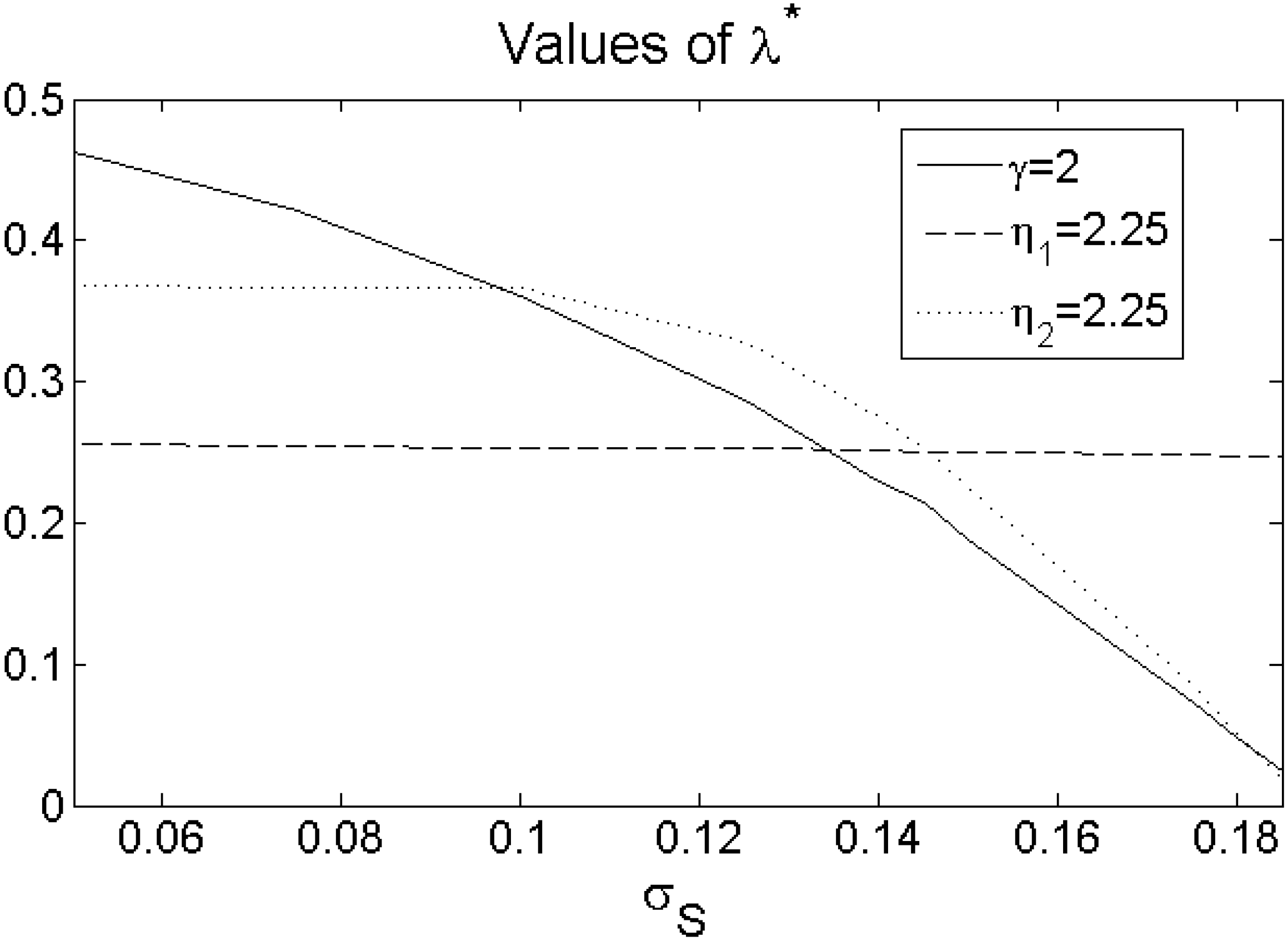
Figure 1. In any case where the indifference parameter exists, the DB plan is preferred for
. Accordingly, it turns out that the salary volatility has a higher and negative impact on the DB plan, which is further discussed in
Figure 1.
Figure 1.
Values for the indifference switching for different levels of the salary volatility .
Figure 1.
Values for the indifference switching for different levels of the salary volatility .
4.1.3. Certainty Equivalents
Another straight means of comparison is to directly compute certainty equivalents and thus to directly determine which pension plan is preferred for a specific preference. Here, we fix the job switching intensity and compute the ratio of the certainty equivalent of the DB plan over that of the DC plan. A ratio above 1 indicates that the DB plan is relatively preferred to the DC plan and the opposite holds if this ratio is less than 1.
In
Table 3, certainty equivalent ratios are computed given a job switching intensity
. This job switching intensity implies that the beneficiary will, on average, switch jobs six times during his career, which is in line with the empirical findings of [
8]. We notice that in most cases, the DC plan is relatively preferred. Only the least risk-averse power beneficiary relatively prefers the DB plan for any investment strategy. This table also nicely illustrates that portability losses have a considerable negative impact on the relative attractiveness of the DB plan.
Table 3.
Values for the certainty equivalent ratio for .
Table 3.
Values for the certainty equivalent ratio for .
| Utility | Risk aversion | | | | |
| CRRA | | 1.1265 | 1.10881 | 1.0748 | 1.0803 |
| | 0.8651 | 0.8792 | 0.9322 | 1.0053 |
| | 0.6831 | 0.7716 | 0.9268 | 1.1121 |
| LA | | 0.9168 | 0.8539 | 0.7873 | 0.7419 |
| | 0.9250 | 0.8647 | 0.7901 | 0.7415 |
| DD | | 0.9863 | 0.9120 | 0.8645 | 0.9254 |
| | 0.8733 | 0.8151 | 0.8210 | 1.1025 |
4.2. Sensitivity Analysis
In this subsection, we investigate how far the more realistic model setup with a time-varying portability loss size, salary trend and job switching intensity affects the above stated results. As suggested in our model setup, we assume the corresponding parameters to be piecewise constant. Specifically, we consider three time periods, where
. The first 10 years are referred to as the early career, the next 10 years as the mid-career and the last five years as the end of the career. In each case, we let one parameter be time-varying, while keeping the other parameters constant. In
Table 4, we compute the indifference job switching intensity for the more realistic case of hump-shaped portability losses,
i.e., U-shaped portability loss size
β; see [
8], Chapter 4. That is, portability losses are increasing up to the end of the mid-career and reach a maximum there, reflected by the high portability loss size (
), while they are very small at the end of the career, accordingly
. The portability loss size at the early career is assumed to be the same as in our benchmark case,
i.e.,
. We observe that our main results stated above, about the impact of the investment strategy, the effect of the risk aversion and also that DD beneficiaries relatively prefer more DB plans than LA beneficiaries, remain unchanged. More specifically, we observe that the more pronounced portability losses in the mid-career imply that the employee would prefer the DC plan after one or two less job moves on average for any utility function. This further indicates that portability losses play a considerable role in the relative attractiveness of the DB plan.
In
Table 5, we compute the indifference job switching intensities for a piecewise constant and time-decreasing salary trend. Specifically, we assume that the employee’s salary growth has the highest trend in the early career
2.25%, and then, this trend decreases gradually in the mid-career (
1.75%) and the late career (
1%). With a piecewise constant and time-decreasing salary drift, we can capture the often,
i.e., for many workers, empirically observed concave shape of the salary curve; see [
8], Chapter 5. The main results observed in our benchmark case of a constant salary drift still carry over. In addition, we see that the higher salary growth rate in the early and mid-career mainly leads to a slight increase in the relative attractiveness of the DB plan. The corresponding economic effects are discussed in the next section in
Figure 2.
Table 4.
Values of for a piecewise constant and U-shaped portability loss size with (original ).
Table 4.
Values of for a piecewise constant and U-shaped portability loss size with (original ).
| Utility | Risk aversion | | | | |
| CRRA | | 0.2721 | 0.2533 | 0.2413 | 0.2441 |
| | 0.1989 | 0.2089 | 0.2431 | 0.2857 |
| | 0.0631 | 0.1268 | 0.2288 | 0.3374 |
| LA | | 0.2503 | 0.2032 | 0.1531 | 0.1102 |
| | 0.2501 | 0.2019 | 0.1528 | 0.1145 |
| DD | | 0.2742 | 0.2447 | 0.2260 | 0.2321 |
| | 0.2360 | 0.2147 | 0.2179 | 0.2583 |
Table 5.
Values of for a piecewise constant and decreasing salary trend with (original ).
Table 5.
Values of for a piecewise constant and decreasing salary trend with (original ).
| Utility | Risk aversion | | | | |
| CRRA | | 0.3500 | 0.3257 | 0.3118 | 0.3148 |
| 0.2601 | 0.2733 | 0.3164 | 0.3692 |
| 0.0974 | 0.1797 | 0.3068 | 0.4370 |
| LA | | 0.3247 | 0.2695 | 0.2032 | 0.1506 |
| 0.3195 | 0.2687 | 0.2021 | 0.1595 |
| DD | | 0.3773 | 0.3324 | 0.2972 | 0.2917 |
| 0.3344 | 0.3050 | 0.2895 | 0.3442 |
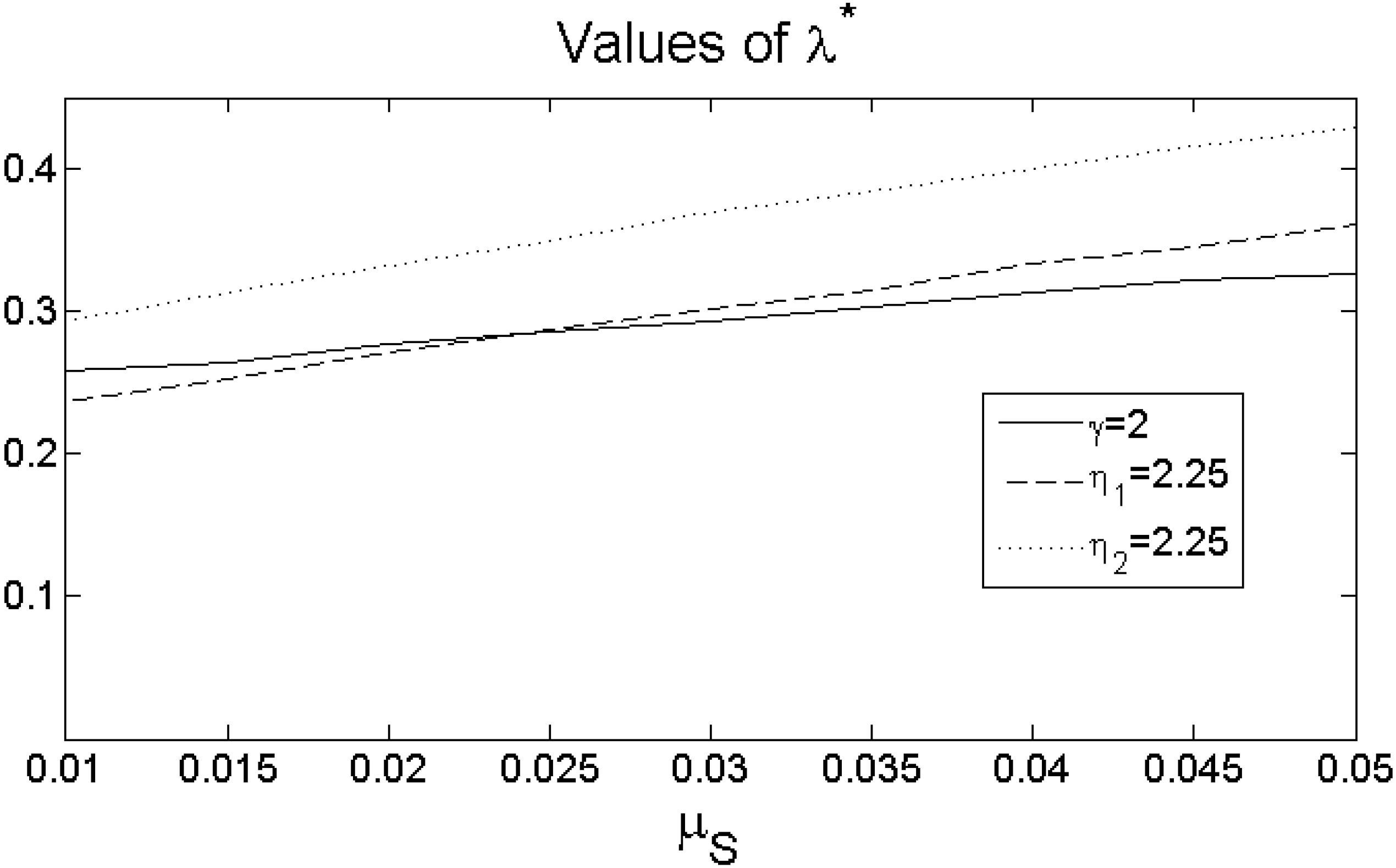
Figure 2.
Values for the indifference switching for different levels of the salary drift .
Figure 2.
Values for the indifference switching for different levels of the salary drift .
As a last robustness check, we consider a deterministic and time-decreasing job switching intensity
λ. It is empirically confirmed that workers change jobs much more frequently when they are younger than when they are older; see e.g. [
24]. Accordingly, we set
. As we have fixed the job switching intensity, we cannot now report the indifference job switching intensity. Therefore, we consider here again the ratio of the certainty equivalents of the DB plan
and that of the DC plan
as the relevant statistic.
Table 6 again confirms our benchmark results. The DC plan remains the beneficial type of plan for most preferences. There is only a slight change for the less loss averse DD beneficiary, since for the suboptimal conservative investment strategy
, this beneficiary would now prefer the DB plan relatively more.
Table 6.
Values for the certainty equivalent ratio for a piecewise constant and decreasing job switching intensity .
Table 6.
Values for the certainty equivalent ratio for a piecewise constant and decreasing job switching intensity .
| Utility | Risk aversion | | | | |
| CRRA | | 1.1707 | 1.1339 | 1.0990 | 1.1153 |
| 0.8974 | 0.9166 | 0.9735 | 1.0419 |
| 0.7119 | 0.8085 | 0.9792 | 1.1695 |
| LA | | 0.9567 | 0.8869 | 0.8227 | 0.7643 |
| 0.9658 | 0.8984 | 0.8333 | 0.7772 |
| DD | | 1.044 | 0.9627 | 0.9117 | 0.9358 |
| 0.9529 | 0.8885 | 0.8829 | 1.1205 |
4.3. Comparative Statics
In the following subsection, we investigate the impact of the crucial contract parameters more closely. To do so, we fix our benchmark investment strategy and set the risk aversion parameters and . We investigate the impact of the salary process, the career length and the employee’s contributions more closely. To better see the effects of the parameters, we consider our benchmark case with a constant salary trend, portability loss size and constant job intensity.
Figure 2 shows values for the indifference job switching intensities
for different levels of the salary drift
. Note first that the employee’s contribution rate
q will be adjusted according to Equation (
12) for each value of
. We observe the standard result in the literature that an increase in the salary drift,
i.e., salary growth rate, makes the DB plan more attractive; see e.g. [
10]. The salary drift has a higher impact on the relative attractiveness of the DB plan for the two utility functions with loss aversion. Intuitively, the impact of the salary drift depends on three effects in our model. First, for any utility function, a higher salary drift implies that it becomes more likely that the beneficiary will receive a higher final salary, which leads to a higher retirement benefit in the DB plan. Second, a higher salary drift also leads to higher contributions in absolute terms in the DC plan. Third, the comparison matching condition (
12) implies that the matched contribution increases with an increase in the salary drift. As the first effect slightly (moderately) dominates, the second and third effect of the DB plan become relatively more attractive for any utility function.
Figure 1 again shows a standard result in the literature. A higher salary volatility decreases the relative attractiveness of the DB pension plan. This is most pronounced for the power utility function; for the LA utility, the salary volatility has a negligible impact, while for the DD utility, the impact becomes fairly pronounced for higher levels of salary volatility. Intuitively, in general, a higher salary volatility makes the final salary more uncertain; in particular, it increases the likelihood of a lower final salary and, thus, of a lower pension benefit. This effect dominates the effect of more uncertain contributions in the DC plan. More specifically, for the LA utility losses,
i.e., shortfalls below the target pension income Rare not severely penalized. This implies that the LA beneficiary almost ignores the higher risk of a loss that comes with an increase of the salary volatility; therefore, the effect of
is negligible for him. For the DD utility, however, losses are penalized more severely; therefore, for higher levels of
(≥10%), an increase also considerably increases the likelihood that the benefits fall below the target pension income. Accordingly, the relative attractiveness of the DB plan substantially decreases for higher values of the salary volatility. Interestingly, there is a critical volatility level, here
15%, where the DD beneficiary prefers the DC plan more than the LA beneficiary. In other words, if the salary risk is very high, the DC plan can become more attractive for the more loss-averse DD beneficiary.
Comparing
Figure 1 and
Figure 2, we can state that the evolution of the salary process affects the DB retirements more than the DC pension retirements. This is intuitive, as the DB formula is solely based on the final salary, whereas the DC pension plan also considerably depends on the investment performance of the financial portfolio.
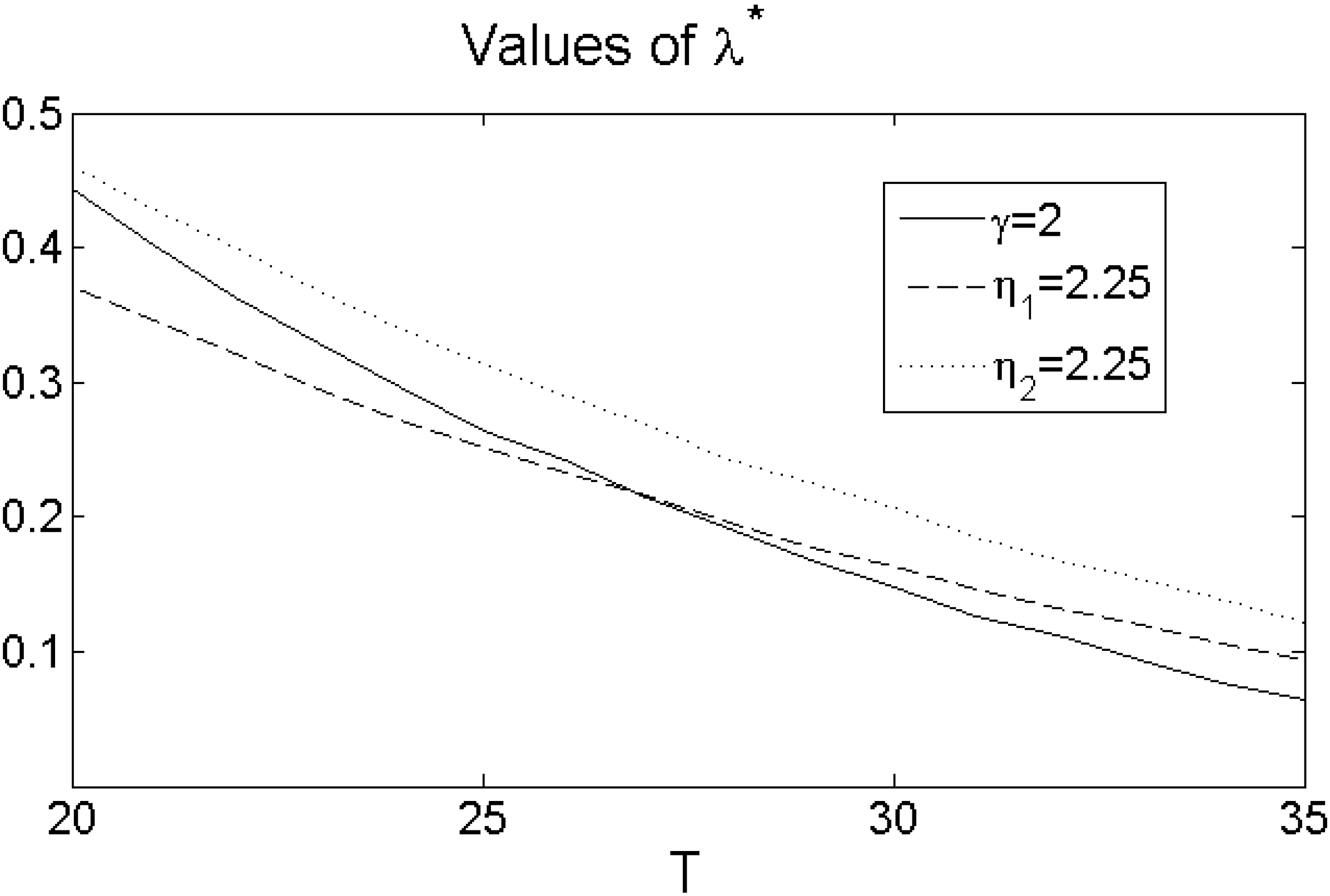
Figure 3.
Values for the indifference switching for different levels of the career length T.
Figure 3.
Values for the indifference switching for different levels of the career length T.
In
Figure 3, we investigate the impact of the career length, or the maturity of the pension retirement contracts, on the relative attractiveness of the two pension retirement plans. A longer (shorter) career length means that the employee enters into the retirement plan when he is younger (older). Again, recall that the employee’s contribution rate
q is computed for each
T according to Equation (
12). One clearly sees that the longer the career length of the employee or the longer the maturity of the pension plan is, the considerably more attractive the DC plan becomes for any utility function. Intuitively, for the older worker, the DB plan is considerably more attractive, since the overall portability loss is also substantially lower. On the other hand, the DC plan is less attractive, because the employee has less time to benefit from the equity premium and to contribute sufficient funds. These two effects substantially dominate the effect that, through the contribution matching condition (
12), the matched contribution rate decreases with the contract maturity. The line of reasoning reverts for the younger employee.
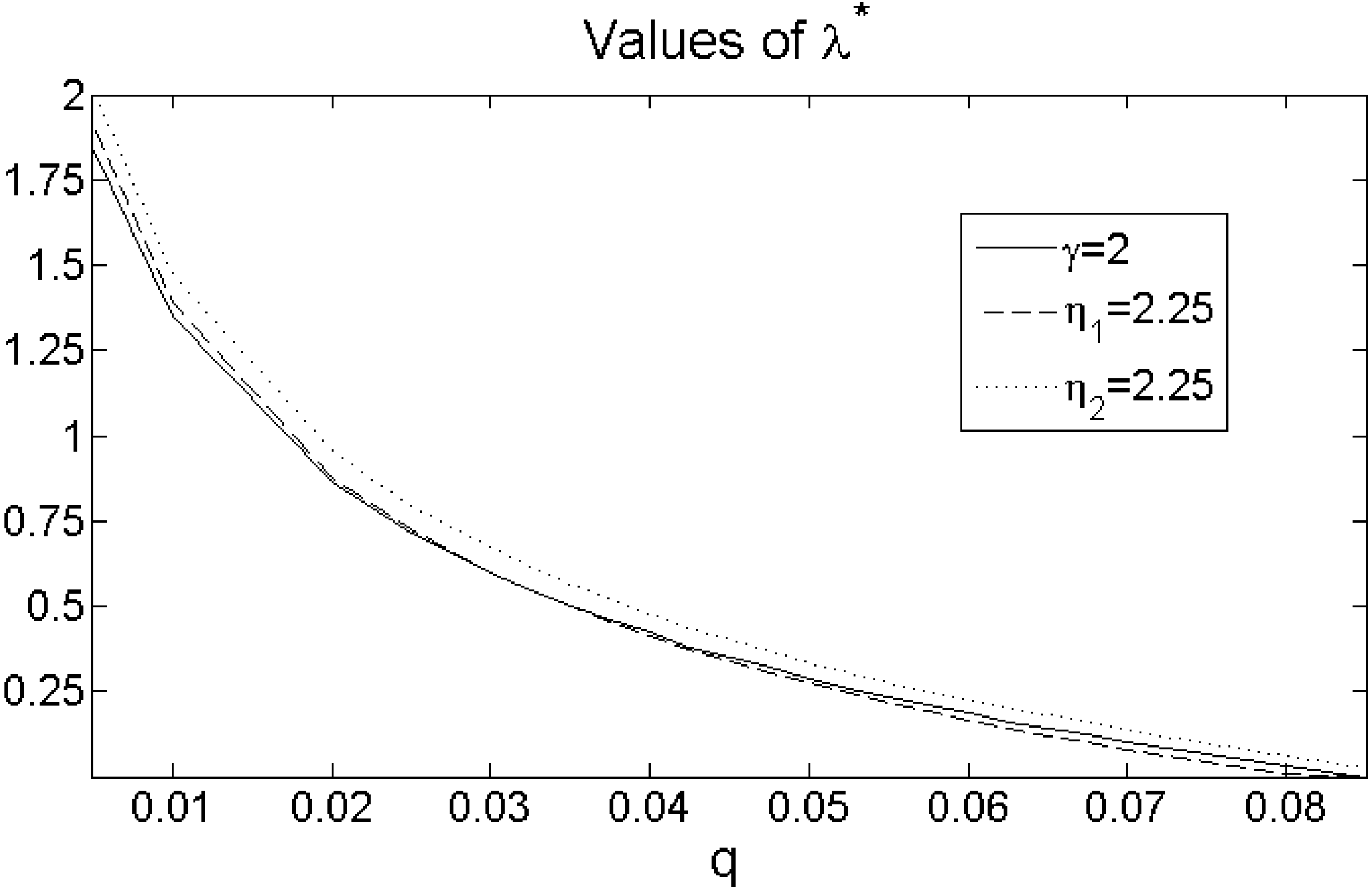
Figure 4.
Values for the indifference switching for different levels of the employee’s contribution rate q.
Figure 4.
Values for the indifference switching for different levels of the employee’s contribution rate q.
Finally, in
Figure 4, we investigate how a change in the employee’s contribution rate
q affects the relative attractiveness of the two pension retirement plans. Therefore, we revert Equation (
12) and compute for each level of
q the corresponding employee’s replacement rate
.
increases in
q for given
. We observe that the DC plan becomes substantially more attractive with an increasing employee contribution rate
q for any utility function, as the effect of a higher contribution dominates the effect of a higher replacement rate. This is particularly the case, because the employer contribution also increases with the employee contribution in the DC pension plan, which is due to the matching mechanism. Most interestingly, we see that for contribution rates, which converge to zero, the DB pension plan is more attractive for any reasonable number of average job moves, while for higher contributions rates,
% the DC plan is always preferred in expected utility terms for any utility function. This result is in line with [
12], who emphasize that, primarily, inadequate contributions lead to retirement incomes that are, on average, lower than the DB counterparts, while adequate contribution rates result in a higher median pension income under the DC plan. [
25] even mentions that a large number of workers eligible for a DC plan fail to contribute. This figure nicely illustrates that for these workers, regardless of their preferences, the DB plan is the better pension plan.
5. Conclusions
The present paper models the most important properties from the beneficiaries’ perspective in DB and DC plans: salary risk present in both the DB and DC plan, portability losses in DB plans due to job switching and asset price risk borne in DC plans. We make comparisons between DB and DC plans by analyzing the expected utility of the pension beneficiary under three preferences: power utility, mean-shortfall and mean-downward-deviation preferences. Most of our findings are consistent with the existing literature. Independent of the preferences, the attractiveness of DB plan increases in the salary growth rate and decreases in the salary volatility and the contract maturity. Our model further indicates that portability losses considerably reduce the relative attractiveness of the DB plan. Moreover, we show that for the utility functions with the loss aversion property, a mean-downside deviation beneficiary prefers the DB plan in most cases relatively more than the mean-shortfall beneficiary. Finally, we have a result that is inconsistent with existing findings. We find that the attractiveness of the DB plan can decrease in the level of risk aversion. This is justified by the fact that the disutility caused by the portability loss (jump risk) can be particularly severe for very risk-averse beneficiaries.
Our paper can be extended by relaxing several assumptions. First, one could also include endogenous or strategic job moves and unemployment in our setup by allowing the salary process to have jumps. Second, the portability risk could be also modeled more realistically by specifying the pension income at retirement as , where denotes the time the employee has worked for employer i. Then, the portability losses could be defined as the difference of a pension income without job moves and the pension income with job moves, i.e., . In this framework, we would link the portability risk to the salary risk and, thus, better capture the major type of portability losses, the cash equivalent losses. Finally, one could allow the beneficiary to have a combination of both a DC and DB pension plan or to change the pension plan at some time in his career.


