
Life Insurance Cash Flows with Policyholder Behavior

1
PFA Pension, Sundkrogsgade 4, DK-2100 Copenhagen Ø, Denmark
2
Department of Mathematical Sciences, University of Copenhagen, Universitetsparken 5, DK-2100 Copenhagen Ø, Denmark
*
Author to whom correspondence should be addressed.
Risks 2015, 3(3), 290-317; https://doi.org/10.3390/risks3030290
Submission received: 16 March 2015
/
Accepted: 5 July 2015
/
Published: 24 July 2015
(This article belongs to the Special Issue Life Insurance and Pensions)
Abstract
:The problem of the valuation of life insurance payments with policyholder behavior is studied. First, a simple survival model is considered, and it is shown how cash flows without policyholder behavior can be modified to include surrender and free policy behavior by calculation of simple integrals. In the second part, a more general disability model with recovery is studied. Here, cash flows are determined by solving a modified Kolmogorov forward differential equation. We conclude the paper with numerical examples illustrating the methods proposed and the impact of policyholder behavior.
1. Introduction
In this paper, we study policyholder behavior in life and pension insurance with a focus on two so-called policyholder options: first, the surrender option, where the policyholder may surrender the contract, canceling all future payments and instead receiving a single payment corresponding to the value of the contract on a technical basis; second, the free policy option1, where the policyholder may cancel the future premiums and have the benefits reduced according to the technical basis. Policyholder modeling has a significant influence on future cash flows. If the technical basis differs considerably from the market basis, policyholder behavior can also have a substantial impact on the market value of the contract.
In a classic Markov chain multi-state life insurance setup, we show how policyholder behavior can be included in cash flow projections. We study two approaches. First, we consider the survival model and show how simple integral expressions can solve the problem. Second, we consider the disability model and present certain ordinary differential equations that solve the problem. This second method has recently been suggested in a more general semi-Markov setup in [1]. We discuss how the integral expressions originating from the survival model can be used to approximate the more correct modeling in the disability model, for a very simple, yet effective type of policyholder behavior modeling.
The policyholder behavior is modeled as random transitions in a Markov model as in [2,3], and the rationality behind surrender and free policy modeling is thus disregarded. An empirical analysis of policyholder behavior in the German market and further references on policyholder modeling can be found in [4]. In contrast, one can consider surrender and free policy exercises as rational, where they purely occur if it is beneficial for the policyholder with some objective measure, see, e.g., [5]. For an introduction to policyholder modeling and a comparison of various approaches, see [6] and the references therein. Attempts to couple the two approaches have been made for surrender behavior, where surrender occurs randomly, but where the probability is somewhat controlled by rational factors, e.g., [7,8]. From a Solvency 2 point of view, the modeling of policyholder behavior is required; see Section 3.5 in [9]. In practice, surrenders and free policy conversions of life insurance contracts are often triggered by external events. Hence, it can be of relevance to study the situation where the policyholder options are exercised randomly, independently of the value of the contract. For example, this might be the case in the labor- and company-based pension insurance market, where the employer or labor organization chooses one pension insurance company for all of their employees or certain groups of their employees; see, e.g., [6]. If one of these employees changes jobs and starts working for a new employer with another pension insurance company, the free policy option will normally be exercised, such that the policyholder stops paying premiums to the original pension company. Similarly, the policyholder may decide to exercise the surrender option and surrender or transfer the contract to the new pension insurance company in order to collect his pension savings in one company.
In the first part of the paper, a simple survival model is considered. We calculate cash flows without policyholder behavior as integral expressions. Then, we extend the model by including first surrender behavior and then both surrender and free policy behavior. We see that these extensions can be obtained via simple modifications of the cash flows without policyholder behavior. This can be viewed as a formula for extending current cash flows without policyholder behavior. However, this modification of the cash flows is only correct for the survival model and not for, e.g., a disability model. If this method is applied to cash flows from a disability model, it could be viewed as an approximation to a more correct way of modeling policyholder behavior. Furthermore, we show that the cash flows with policyholder behavior can be derived from cash flows with surrender behavior. This method can be used in the case where one has access to cash flows with surrender behavior, but not free policy behavior. In practice, many life insurance companies work with cash flows without policyholder behavior; hence, the proposed method may be viewed as a simple alternative to full, combined modeling of policyholder behavior and insurance risk. The quality of these formulae as an approximation is assessed numerically in the last part of the paper. This issue is also studied numerically in [3], where they examine ways to simplify the calculations when modeling policyholder behavior.
In the second part, we consider the more correct way of modeling policyholder behavior in a multi-state life insurance setup. This model is presented in [1] for the general semi-Markov setup, and here, we present the special case of a Markov process for the disability model with recovery. Within this setup, the transition probabilities are first calculated using Kolmogorov’s forward differential equation, and then, the cash flow can be determined. When including policyholder behavior, duration dependence is introduced, since the future payments are affected by the time of the free policy conversion. This complicates calculations significantly, since it becomes necessary to determine the joint distribution of the Markov process and the time of the free policy conversion in order to calculate the cash flows. In practice, we would have to solve partial instead of ordinary differential equations. We present the main result from [1] that allows us to effectively dismiss the duration dependence and to calculate cash flows with policyholder behavior by simply calculating a slightly modified version of Kolmogorov’s forward (ordinary) differential equation. The complexity of the calculations is therefore not increased significantly by inclusion of policyholder behavior.
In the third part of the paper, a numerical example is studied, which illustrates, in part, the importance of including policyholder modeling when valuating cash flows and, in part, the quality of the approximating cash flows obtained by applying the integral expressions from the first part to cash flows without policyholder behavior from a disability model. We see that the structure of the cash flows changes significantly in our example, and the dollar duration measuring interest rate risk is reduced by about 66%, when including policyholder behavior. For hedging of interest rate risk, it is thus essential to consider policyholder behavior. We compare the approximate method with the correct approach of solving the modified Kolmogorov differential equations and find cash flows with policyholder behavior in a disability model. We find that in our example, the approximation is very precise. In the last part of the numerical study, we have exploited the main result of the paper and solved our modified version of Kolmogorov’s forward differential equations numerically.
Since the results obtained in the second part of the paper can be viewed as a special case of the ones presented in the more general semi-Markov framework in [1], we briefly describe the main differences between the two presentations. As mentioned above, in [1], the Kolmogorov forward integro-differential equation in the semi-Markov framework is studied, and a modified version is presented that allows for the inclusion of policyholder behavior in an efficient manner. The present paper contains three parts. In the first part, we discuss a simple approach to modeling policyholder behavior, which is based on a modification of the underlying cash flows without policyholder behavior. This construction provides simple pedagogical interpretations for the various new terms that arise in the cash flows when we introduce policyholder behavior. Similar results are presented in [3], who compare with alternative modifications of the cash flows in more abstract models, such as the disability model. The second part presents the modified Kolmogorov equation in the classic Markov model. We believe that the presentation in this part could be accessible to a wider audience than [1], since we can avoid the more technical issues related to the semi-Markov framework with duration dependence. This leads to simpler results that are more easy to interpret, implement and more directly applicable than the semi-Markov framework. Moreover, the proofs are more direct and should be easy to follow for readers familiar with the classic Markov models as presented in, e.g., [10].
2. Life Insurance Setup
The general setup is the classic multi-state setup in life insurance, consisting of a Markov process, Z, in a finite state space indicating the state of the insured; see [11]. We associate payments with sojourns in states and transitions between states, and this specifies the life insurance contract. We go through the setup and basic results; for more details, see, e.g., [6,10,12].
Assume that Z is a Markov process in and that . The transition probabilities are defined by:
for and . Define the transition rates, for ,
We assume that these quantities exist. Define also the counting processes , for , , counting the transitions between state i and j. They are defined by:
where we have used the notation .
The payments consist of continuous payment rates during sojourns in states and single payments upon transitions between states. Denote by the payment rate at time t if , and let be the payment upon transition from state i to j at time t. Then, the accumulated payments at time t are denoted and are given by:
Positive values of the payment functions and correspond to benefits, while negative values correspond to premiums. It is also possible to include single payments during sojourns in states, but that is, for notational simplicity, omitted here.
We assume that the interest rate is deterministic. Then, the present value at time t of all future payments is denoted , and it is given by:
The formula is interpreted as the sum over all future payments, , which are discounted by . For a current valuation, we take the expectation conditional on the current state, . This expected present value is called the prospective (state-wise) reserve.
Definition 1. The prospective reserve at time t for state is denoted and given as:
The prospective reserve can be calculated using the following classic results.
Proposition 1. The prospective reserve at time t given , , satisfies,
Proposition 2. The prospective reserve at time t given , , satisfies Thiele’s differential equation,
with boundary conditions , for .
Proof. See Formula (4.7) in [11]. ☐
Remark 1. If a time point exists, such that for and all , then the boundary conditions for are used with Thiele’s differential equation.
It can be convenient to calculate not only the expected present value (the prospective reserve), but also the expected cash flow. From here on, we simply refer to the expected cash flow as the cash flow, and it is a function giving the expected payments at any future time s. The cash flow is, in this setup, independent of the interest rate, and thus, the cash flow can be useful for hedging and for an assessment of the interest rate risk associated with the life insurance liabilities.
Definition 2. The cash flow at time t associated with the payment process , conditional on , , is the function , given by:
for .
A formal calculation yields an expression for the cash flow: from Definition 1, we note that:
where we have used that is a constant and does not change the dynamics in s. We state the result in a proposition.
Proposition 3. The cash flow satisfies,
Proof. The first result is proven in Proposition 2.3 in [1] using integration by parts. The second result follows from the first result and from Proposition 1. ☐
In order to actually calculate the cash flow, one must first calculate the transition probabilities . In sufficiently simple models, the so-called hierarchical models, where you cannot return to a state after you have left it, the transition probabilities can be calculated using only integrals and known functions. These kind of models are considered in Section 3. In more general Markov models, closed form expressions for the transition probabilities typically do not exist, except for certain cases when the transition rates are piecewise constant. Usually, the transition probabilities are found numerically by solving Kolmogorov’s forward or backward differential equation.
Proposition 4. The transition probabilities , for , are unique solutions to Kolmogorov’s backward differential equation,
with boundary conditions and Kolmogorov’s forward differential equation,
with boundary conditions .
Proof. See [10], Theorem 2.3.4. ☐
Using Kolmogorov’s differential equations, the transition probabilities needed in order to calculate the cash flow from Proposition 3 can be found. It is worth noting that for calculating the cash flow, using the forward differential equation is the easiest way to obtain the desired transition probabilities.
Remark 2. The payments are for notational simplicity assumed to be continuous throughout the paper. It is straightforward to include single payments at deterministic time points, which allows for, e.g., an endowment insurance. For example, if a single state-dependent payment at time T is included, , Formula (1) would read:
where is the point measure at T. In that case, the cash flow from Proposition 3 would read:
2.1. Technical Basis and Market Basis
In practice and in our examples, we distinguish between calculations on the so-called technical basis, used to settle premiums, and the market basis, used to calculate the market consistent value of the life insurance liabilities, referred to as the market value. A basis is a set of assumptions used for the calculations of life insurance liabilities, and it typically consists of an interest rate and a set of transition rates . There can also be different administration costs associated with different bases; however, administration costs are not considered in this paper. The Markov model can also be different in different bases, and the policyholder behavior modeling of this paper is an example of this. Here, policyholder behavior is not included in the technical basis, but is included in the market basis, so the Markov models differ by the surrender and free policy states.
Throughout the paper, we let and be the first order interest and transition rates, respectively, i.e., the interest and transition rates associated with the technical basis. We let and be the interest and transition rates, respectively, for the market basis. In general, values marked with a ^ are associated with the technical basis. Thus, is the prospective reserve for the market basis, and is the prospective reserve for the technical basis.
2.2. The Policyholder Options
We study life insurance contracts with two options for the policyholder. She can surrender the contract at any time or she can stop the premium payments and convert the policy into a so-called free policy.
If the policyholder surrenders the contract at time t, all future payments are canceled, and instead, the policyholder receives compensation for the premiums she has paid so far. Usually, the prospective reserve calculated on the technical basis, , is paid out, but the formula allows it to be any deterministic value. In this paper, we allow for a deductible and say that the payment upon surrender is . Since any deterministic value can be chosen, in particular, we can choose κ to be time dependent.
If the policyholder stops the premium payments, i.e., exercises the free policy option, all future premiums are canceled, and the size of the benefits is decreased to account for the missing future premium payments. In this paper, we assume that the free policy conversion can only occur from State 0. If the free policy option is exercised at time t, all future benefits are decreased by a factor . In order to handle this, we split the payment process into positive and negative payments, corresponding to benefits and premiums, respectively. The benefit and premium cash flows are denoted by and , respectively, and are given by:
where the notation and for a function is used. The prospective reserve can then be decomposed, as well, and we have:
and . The relations also hold on the technical basis; thus, , where and are the values of the future benefits and premiums, respectively, valuated on the technical basis.
If the free policy is exercised at time t, then at a future time s, the payment rate while in state i is , and the payment if a transition from state i to j occurs is . Hence, the prospective reserve on the technical basis at time s in state i, given the free policy option is exercised at time , is:
where is the cash flow calculated with the first order transition probabilities and rates, determined by .
We recall that free policy conversion can only occur from State 0, and from here on, we generally omit the subscript 0 from, e.g., when there is no ambiguity. The free policy factor should be deterministic and is usually chosen according to the equivalence principle on the technical basis: the prospective reserve for the technical basis should not change as a consequence of the exercise of the free policy option. If we assume the free policy conversion is exercised at time t, the prospective reserve on the technical basis before the conversion, , should be equal to the prospective reserve after conversion, . Thus, we require , yielding:
We see that ρ is the value on the technical basis of benefits less premiums, divided by the value on the technical basis of the benefits only. We refer to as the free policy factor.
3. The Survival Model
We consider the survival model and extend it gradually to include policyholder behavior. First, we include the surrender option, and afterwards, we include the free policy option, as well. The survival model consists of two states, 0 (alive) and 1 (dead), corresponding to Figure 1.
Figure 1.
Survival Markov model.

Assume the insured is x years old at Time 0. The payments consist of a benefit rate and a premium rate , as well as a payment upon death at time t. Referring to the general setup, we have:
and also, we denote the mortality intensity . The prospective reserve on the technical basis at time t in State 0 is given by Proposition 1, and we get:
We have used the actuarial notation for the survival probability, , and it is given by,
Thus, is the survival probability of an x-year old reaching age , calculated on the technical basis.
The market values of benefits and premiums, respectively, are then given by:
and the associated cash flows, conditioning on being alive at time t, are:
with and being the total prospective reserve and cash flow, respectively. Here, we have omitted the subscript 0 from the notation .
The free policy factor is determined by:
where is the value on the technical basis of the benefits only. If the free policy option is exercised immediately, the market value is:
and in Denmark, this is often referred to as the market value of the guaranteed free policy benefits.
3.1. Survival Model with Surrender Modeling
We continue the example from above and determine the market value including the valuation of the surrender option. The Markov model is extended to include a surrender state, corresponding to Figure 2.
The surrender modeling is only included in the market basis, and the valuation on the technical basis does not change. This is reasonable, since if the technical reserve is paid out upon surrender, modeling the surrender option on the technical basis does not affect the value of the technical reserve. If the surrender value differs from the technical reserve, one should also model the surrender option on the technical basis when setting premiums. This can be handled with the results of the present paper, since they hold for any deterministic surrender payments.
Figure 2.
Survival Markov model with surrender.

On the market basis, we denote the surrender rate by . We introduce a quantity , which is the probability that an x-year old does not die, nor surrender before time . It is thus the probability of staying in State 0 and is given by,
Here, the transition rates and are for an x-year old at Time 0, which for simplicity, is suppressed in the notation.
The payment upon surrender at time s is , and the cash flow valuated at time t is, by Proposition 3,
We decompose the cash flow in all payments excluding the surrender payments,
and the surrender payments,
Here, is the cash flow from the model in Figure 1, as defined by Equation (2). The market value calculated on the market basis including surrender is denoted and is given by:
We see that the cash flow and market value including surrender modeling are found using the original cash flow without surrender modeling, , and multiplying the probability of no surrender . Thus, finding the cash flow and the market value in the survival model with surrender is particularly simple when the existing cash flow is known.
3.2. Survival Model with Surrender and Free Policy Modeling
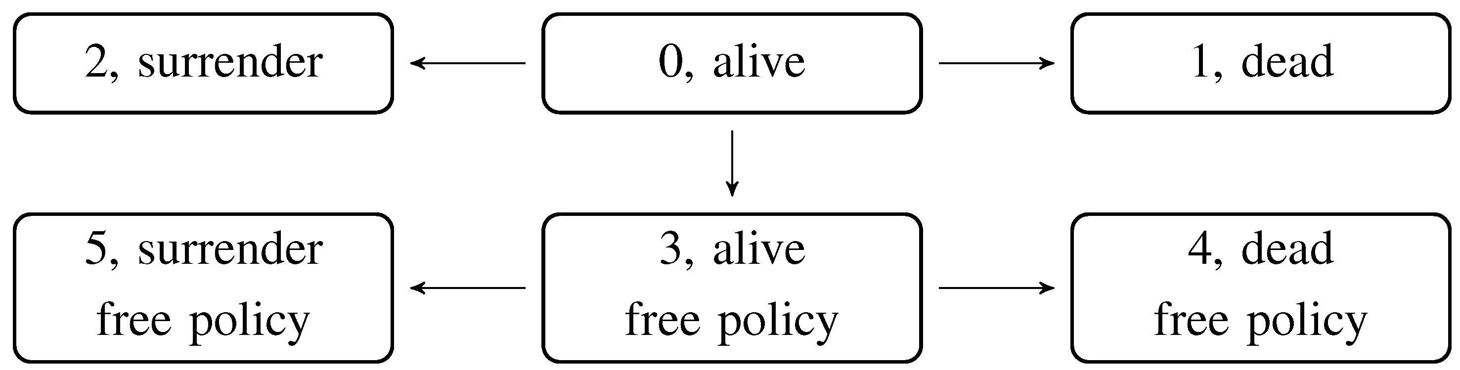
We extend the model to include free policy modeling on the market basis, and the Markov model is extended in Figure 3 to include free policy states. The mortality and surrender transition rates in the free policy states are identical to those in the premium paying states, and .
Figure 3.
Survival Markov model with surrender and free policy.

We introduce a free policy rate , which is the transition rate of becoming a free policy at time t. We introduce the notation:
which is the probability of staying in State 0, i.e., not becoming a free policy, surrendering nor dying.
If the free policy transition occurs at time t, the future benefits are reduced by a factor , and the future premiums are canceled. Thus, in the free policy state at a later time s, the payment rate is , and the payment upon death is . The surrender payment, if surrender occurs as a free policy, is , where is the prospective reserve on the technical basis.
The payment process is dependent on the exact time of the free policy transition, i.e., the payments are dependent on the duration since the free policy transition. It can be shown that the cash flow valuated at time t is given by:
The result can be obtained as a special case of Proposition 5 below, where the disability rate is set to zero, but for completeness, a separate proof is given in Appendix A.1. The first line is the payments in State 0 and the payments upon death and surrender. The second and third lines contain the payments as a free policy. This expression can be interpreted as the probability of staying in State 0 until time τ, then becoming a free policy at time τ and then neither dying nor surrendering from time τ to time s. This is multiplied with the payments as a free policy at time s, given the free policy occurred at time τ. Finally, we integrate over all possible free policy transition times from s to t.
The cash flow is decomposed into four parts. First, the benefits and premiums, excluding surrender payments, while alive and not a free policy,
Then, the surrender payments, if the free policy transition has not occurred,
Note that these cash flows correspond to the cash flows in the surrender model, but reduced with the probability of the free policy transition not happening.
The third cash flow is the benefits while a free policy:
and the fourth cash flow is the surrender payments while a free policy,
The third cash flow Equation (8) seems complicated, since the cash flows at time s evaluated at time τ, , are needed for any and all . However, a straightforward calculation yields,
which simplifies things, and insertion of this into yields,
Define the quantity:
and note that:
The market value including surrender and free policy modeling is denoted , and it may finally be written as:
The last four lines in Equation (11) have the following interpretation.
- The first line is the value of the original cash flow Equation (2) without policyholder behavior, reduced by the probability of not surrendering and not becoming a free policy.
- The second line is the value of the surrender payments, when not a free policy.
- The third line is the benefit payments as a free policy, i.e., the positive payments reduced with the free policy factor at the time τ of the free policy transition.
- The fourth line is the surrender payments if surrender occurs after the free policy transition.
The formula gives the market value of future guaranteed payments, including valuation of the surrender and free policy options. In order to calculate the value, the following quantities are needed:
- The original cash flows and .
- The prospective reserve on the technical basis and , for all future time points , which allow us to determine the surrender payments and the free policy factor .
- The factor , which is a simple integral of the free policy transition rate.
3.3. Free Policy Modeling When Surrender Is Already Modeled
In the previous section, we found the market value including surrender and free policy modeling based on cash flows without any policyholder behavior modeling. It is also possible to find this market value based on cash flows including surrender modeling. This could be relevant if the existing cash flows already include surrender modeling and one wishes to modify these cash flows to include free policy modeling. Thus, we assume that the cash flows including surrender behavior modeling, Equation (3), are available, and that these are split into a cash flow associated with the benefits and a cash flow associated with premiums, i.e.,
Note that the payment upon surrender is split between the two cash flows, through the decomposition , i.e., the value of the future benefits less the value of the future premiums.
The market value with surrender modeling, but not free policy modeling, from Equation (4), is then given by:
We find the cash flow including free policy modeling by modifying the existing cash flows into two cash flows: one, which is reduced by the probability of not becoming a free policy, and a special free policy cash flow. With a few calculations using Equations (6), (7) and (12), we see that:
and also, by Equations (8)–(10) and (12),
The total cash flow is then given as:
This cash flow can be interpreted as a weighted average between the original cash flow, reduced with the probability of not becoming a free policy, and the payments as a free policy. The payments as a free policy are the positive payments multiplied with . The quantity is interpreted as the probability of becoming a free policy multiplied with the free policy factor at the time τ of the free policy transition.
The market value from before, , can then be calculated as:
If we only include surrender modeling, the needed extra quantities are simple integrals of the surrender rate . If we in addition include free policy modeling, the free policy factor must also be found, which requires access to future prospective reserves on the technical basis. When these are found, the market value is relatively simple to calculate.
3.4. Approximate Method
An essential assumption for these calculations is that there are no payments after leaving the active state, i.e., that the prospective reserve is zero in the dead and surrender states. That is, after the payment upon
death or surrender, there are no future payments. If one adds a disability state, similar simple results can only be obtained if the prospective reserve is zero in the disability state. This is typically not satisfied, and as such, the methods of modifying the cash flows presented here are not applicable. However, assuming one has cash flows from a more general model without policyholder behavior (e.g., a disability model), Formula (11) can be applied to these cash flows in order to obtain an approximation to cash flows with policyholder behavior. We refer to this method as the approximate method.
In the following section, we examine how to correctly model policyholder behavior in a disability Markov model.
4. A General Disability Markov Model
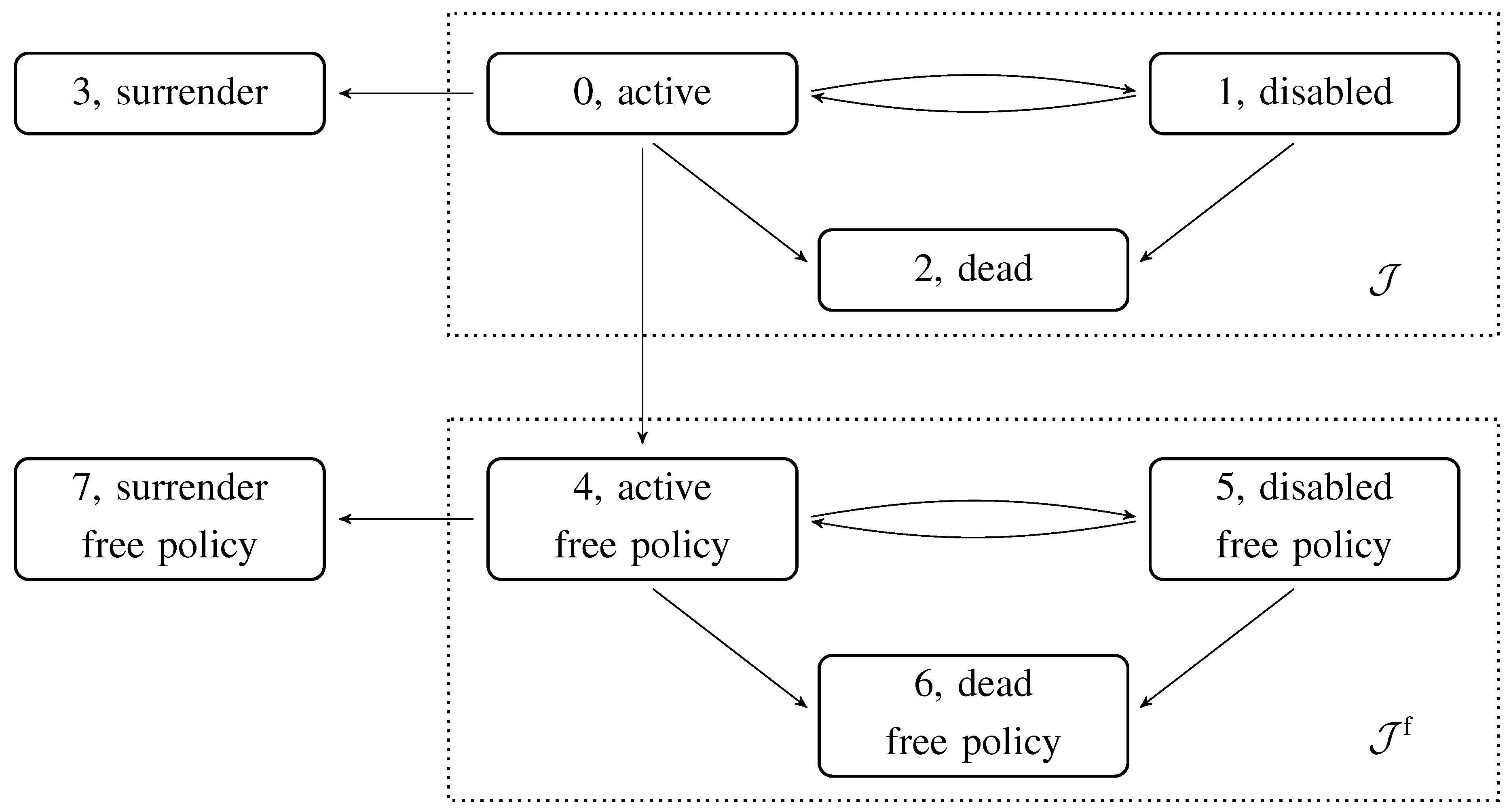
In this section, we consider the survival model extended with a disability state, from which it is possible to recover. We extend the model further by including states for surrender and free policy and end up with an eight-state model; see Figure 4. By solving certain ordinary differential equations for the relevant transition probabilities and a special free policy quantity, similar to from Equation (10), the cash flow and prospective reserve can be found.
Figure 4.
The eight-state Markov model, with disability, surrender and free policy. The transition rates between States 0, 1 and 2 are identical to the transition rates between States 4–6. The two surrender states can be considered one state, and then, this model is known as the so-called “seven-state model”.

The results can easily be extended to more general Markov models than the disability model, as long as free policy conversion only occurs from the active State 0. A more general setup is studied in [1], which is here specialized to the case of the survival-disability model.
For valuation on the technical basis, the survival-disability Markov model, consisting of States 0, 1 and 2, is used. In this section, the payments are labeled by the state they correspond to instead of the labels used previously. Thus, the payment rate in State 0, active, is , and in State 1, disabled, it is . Upon disability, there is a payment ; upon death as active, there is a payment ; and upon death as disabled, there is a payment . The payment function in State 0, , is decomposed into positive payments , which are benefits, and negative payments, , which are premiums. Thus,
We assume that all other payments functions are positive. The notation corresponds to the notation used in Equation (1) for the payment functions , , , and , and all other payment functions and are zero. The transition rates are also labeled by numbers, e.g., the transition rate from state i to j is .
Using Proposition 3, the cash flow for State 0 under the technical basis is,
where the notation and refers to the transition probabilities and rates on the technical basis. The first line contains payments while in State 0, active, and payments during transitions out of State 0. The payments on the second line are payments in State 1, disabled, and payments during transitions out of State 1. We decompose the cash flow into positive and negative payments and define,
such that . The prospective reserve on the technical basis is also decomposed,
and we have . Here, we again omit the notation 0 for the state in the reserves and cash flows.
For valuation on the market basis, we consider the extended Markov model in Figure 4. We define a duration, , which is the time since the free policy option was exercised (or since surrender),
If the free policy option is exercised and the current time is t, the time of the free policy transition is then . Upon transition to a free policy, the benefits are reduced by the factor , and the premiums are canceled. The payments in the free policy states are thus duration dependent, and at time t, they are,
Upon surrender from State 0, an amount is paid out, where is the prospective reserve on the technical basis. If the free policy option is exercised and surrender occurs from State 4, the prospective reserve on the technical basis is the value of the future benefits, reduced by the free policy factor . Thus, the payment upon surrender as a free policy is . The parameter κ is a surrender strain and is usually zero. We have,
The total payment process is then given by,
The first two lines contain the benefits and premiums in the States 0, alive, 1, disabled, and 2, dead. Line 3 contains the payment upon surrender as a premium paying policy, and Line 6 contains the payment upon surrender as a free policy. Lines 4 and 5 contain the payments as a free policy.
We find the cash flow, and to this end, it is convenient to define the quantity:
for , , and . Then, it holds that:
For a proof of Equation (14), see Appendix A.2. For , this quantity is simply the transition probability from state i to j: it is the probability of going from State i to 0 at time τ and then transitioning to State 4 at time τ and, finally, going from State 4 to State j from time τ to s. Since a transition from a state to a state can only occur through a transition from State 0 to 4, this gives the transition probability. When , the quantity corresponds to the transition probability multiplied by at the time of transition to a free policy.
We now state the cash flow.
Proposition 5. The cash flow in State 0, , for payments at time s valued at time t, is given by:
Proof. See Appendix A.3. ☐
Calculation of the cash flow requires to be calculated, and with Equation (14), this requires the transition probabilities for all s and τ satisfying . However, it turns out that this is not necessary, since there exists a differential equation for similar to Kolmogorov’s forward differential equation. Using this, one can calculate all of the usual transition probabilities and the quantities together. This eliminates the need to calculate for all τ and s satisfying .
Proposition 6. The quantities satisfy the forward differential equation, for and ,
with boundary conditions .
Proof. See Appendix A.4. ☐
A more general version of this result is presented in Theorem 4.2 in [1] for the general semi-Markov case and can also be found for the general Markov case as Equation (4.8) in [1]. However, for completeness, a straightforward proof is given in the Appendix. For the proposition, we recall that is the sum of all of the transition rates out of state j. Note, in particular, that if , the last sum is simply the one term and if , the last term is .
The market value including surrender and free policy modeling is denoted and is given by,
The first three lines are the payments when the free policy option is not exercised, and the last three lines are payments as a free policy. The first two lines are the payments without policyholder behavior, which is similar to the first line in Equation (11). The third line is the surrender payments when the free policy option is not exercised, and this is similar to Line 2 in Equation (11). The fourth and fifth lines are the payments as a free policy, without the surrender payment, corresponding to the third line in Equation (11). The last line is the surrender payments as a free policy, which corresponds to the fourth line in Equation (11). If the disability state is removed, the formula simplifies to Equation (11).
Remark 3. In Remark 2, single payments at time T were allowed. This can be included in the above results: if we assume single payments at time T, in state alive and in state disabled, the following terms must be added to the cash flow Equation (15),
As a consequence, the following terms must be added to the market value Equation (16),
5. Numerical Example
We present a numerical example that illustrates the methods presented in the previous sections. First, we illustrate the impact of modeling policyholder behavior, and in particular, we see that the structure of the cash flows changes considerably. With the modeling of policyholder behavior, the interest rate sensitivity (duration) of the cash flow is significantly reduced, which is of importance if one applies duration matching techniques in order to hedge the interest rate risk.
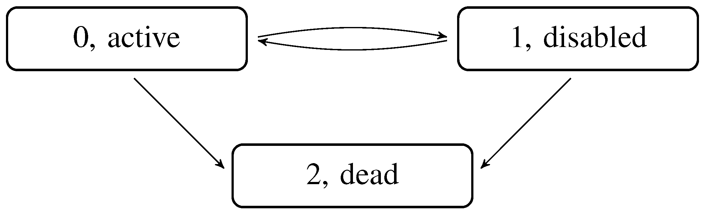
Second, we illustrate the error when using the simple model from Section 3.1 to modify existing cash flows from a disability model to include policyholder behavior. In Section 3.1, it is shown how to manipulate cash flows from a life-death model to include policyholder behavior according to the model shown in Figure 3. When using the methods on cash flows originating from the three-state disability model shown in Figure 5, the formulae do not give the correct result, but they can serve as an approximation to the full model from Figure 4. As illustrated in this example, it can indeed be a very good approximation.
Figure 5.
Disability Markov model.

We consider a 40-year-old male now at Time 0, with retirement age 65. He enters a new policy with two products:
- A disability annuity consisting of an annual payment of 100.000 while disabled, until age 65.
- A life annuity consisting of an annual payment of 100.000 while alive, from age 65 until death.
He pays a yearly premium while active, determined by the principle of equivalence on the technical basis. The principle of equivalence states that the prospective reserve on the technical basis is zero before any payments are made. The technical basis consists of:
- The three-state disability Markov-model, as shown in Figure 5;
- Interest rate of 1%;
- Transition rates, where x is the age,
The transition rates are designed such that we do not distinguish between disabled and active after retirement; thus, the mortality rate as disabled is simply set to the mortality rate as active after age 65, and this is simply interpreted as the average mortality rate from alive to dead.
With the technical basis and the equivalence principle, the premium paid while active is found to be of annual size 46.409 until age 65. Using the technical basis, we also find the technical reserve at future time points for the active and the free policy state. This determines the surrender payments and the free policy conversion factor, which are needed for the calculations below.
For the market basis, the interest rate provided by the Danish FSAof 2 September 2013 is used. The transition rates loosely resemble those used by a large Danish life and pension insurance company in the competitive market. With x being the age, they are given by,
- active to dead, : the mortality benchmark from 2012 from The Danish FSA,
- active to disabled: ,
- disabled to active: ,
- disabled to dead: .
The active to surrender (as), respectively to free policy (af), transition rates are for age given as
and they are set to zero for .
The transition rates are shown in Figure 6 together with the transition probabilities, which have been calculated using Kolmogorov’s forward differential equation, Proposition 4. The probability of surrender and free policy conversion are significant, and already around age 47, the probability of having surrendered or made a free policy conversion is greater than the probability of still being active. We also note that the transition probabilities are smooth except at age 65, where the disability, recovery, surrender and free policy transition rates jump to zero.
Figure 6.
Transition rates (left) and transition probabilities (right). In the left figure, the transition rates between the states in the disability model, (0, active, 1, disabled, and 2, dead) are shown, as well as the surrender (active to surrender (as)) and free policy (active to free policy (af)) transition rates. In the right figure, the full lines are the non-free policy states, and the dashed lines are corresponding free policy states. The active, free policy and surrender states are dominant.

Figure 7.
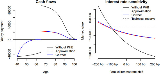
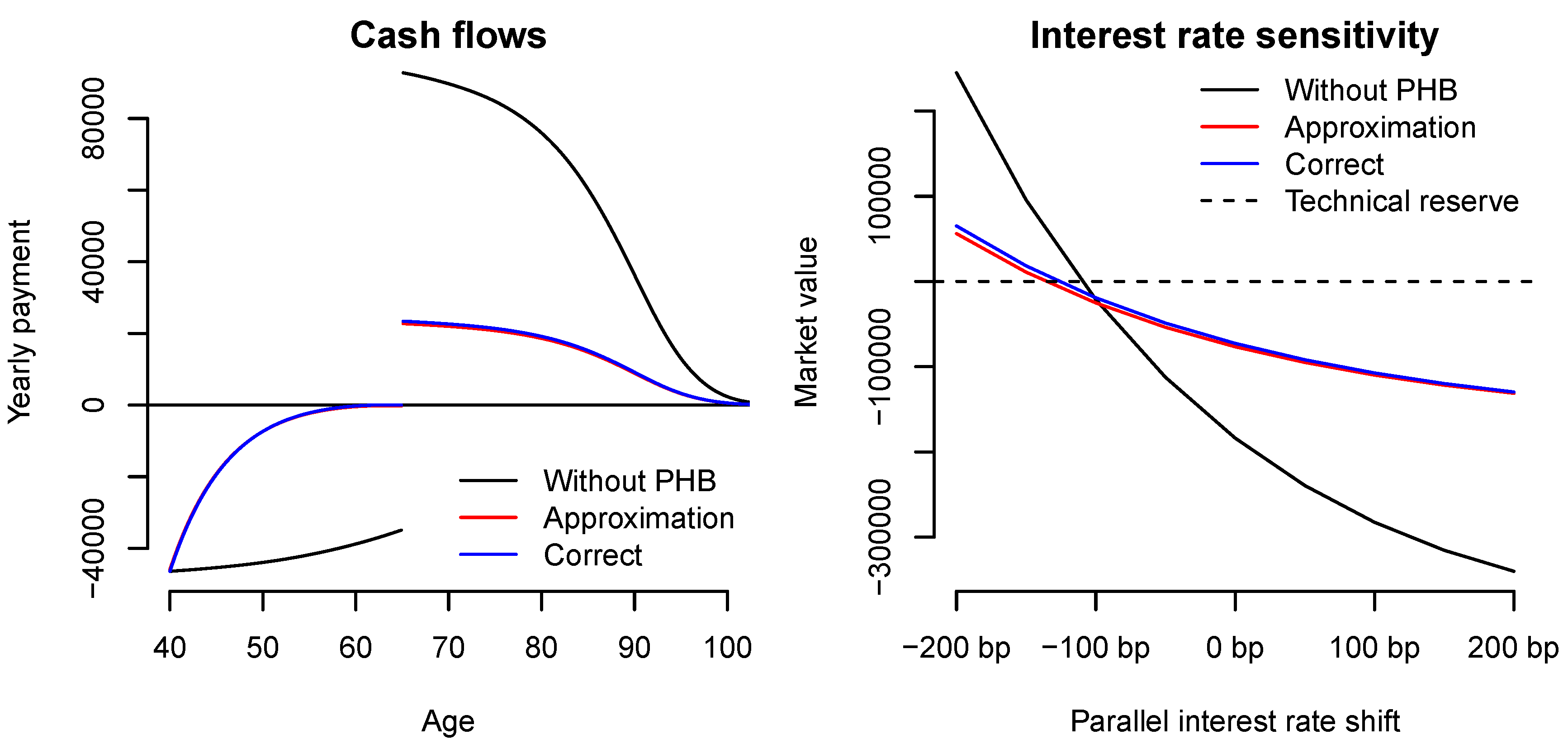
Cash flows (left) and market value for different parallel shifts in the interest rate structure (right), measured in basis points. In the figures, we see that the modeling of policyholder behavior has a major impact. Furthermore, it seems difficult to distinguish the approximate and the correct method using the eye-ball norm only. The approximation yields a slightly larger cash flow and market value than the correct modeling does.
Figure 7.
Cash flows (left) and market value for different parallel shifts in the interest rate structure (right), measured in basis points. In the figures, we see that the modeling of policyholder behavior has a major impact. Furthermore, it seems difficult to distinguish the approximate and the correct method using the eye-ball norm only. The approximation yields a slightly larger cash flow and market value than the correct modeling does.

We perform three calculations. First, we consider the disability model without policyholder behavior, as shown in Figure 5. In this model, the cash flow and the corresponding market value are calculated, using Propositions 3 and 4. In Figure 7, these results are shown as the black lines. In the beginning, the premiums are paid, and the cash flow starts at the annual premium level −46.409. If the insured dies, the premium stops, and upon disability, the premium stops and the disability annuity is paid. Thus, we see a slightly increasing cash flow until age 65. After retirement, a life annuity is paid out instead. The value of the cash flow at age 65 is slightly less than 100.000, corresponding to a strictly positive probability of death before age 65. The cash flow decreases to zero as the insured eventually dies.
In Table 1, the market value and the dollar duration are presented. The technical reserve is zero due to the equivalence principle, corresponding to this being a new policy. The market value is negative, which expresses a surplus inherent in the contract, because the technical basis is on the safe side. We see that the dollar duration is significant, and from Figure 7, it is seen that a decrease of a little more than 100 basis points in the interest rate leads to an increase in the market value, eliminating the surplus completely.

Table 1.
Market value of the cash flow and dollar durations (DV01), without policyholder behavior (PHB), with the approximative method and the correct method. The duration is greatly reduced when policyholder behavior is included, and the approximation is close to the result from the correct method.
| Results | Without PHB | Approximation | Correct |
|---|---|---|---|
| Market value | −183.798 | −76.599 | −72.641 |
| DV01 | 130.792 | 42.462 | 44.239 |
For the second calculation, we consider the approximate method, as discussed in Section 3.4. The cash flow without any modeling of policyholder behavior, , is modified by Formula (11) in order to obtain approximate cash flows including policyholder behavior. As mentioned above, this is only correct if the cash flows originate from a two-state survival model, as shown in Figure 1. However, we perform the modification anyway and examine the quality of this as an approximation. One can show that this calculation corresponds to allowing surrender and free policy from the disability state; see [3]. In Figure 7, the results from this modification are shown as the red lines.
As mentioned above, free policy modeling leads to duration-dependent payments, since the payments in the free policy states depend not only on the current state, but also on the time of the free policy conversion. This implies that one would need to determine the joint distribution of the Markov process and of the time of free policy conversion in order to calculate the cash flows correctly, which in practice amounts to solving a partial differential equation. In the numerical calculations for this study, we have used Propositions 5 and 6 from Section 4 and correctly calculated the cash flows, where surrender and free policy conversion are only possible from the active states. By these results, we simply solved ordinary differential equations. In Figure 7, this is shown as the blue lines.
We see that including modeling of policyholder behavior has an effect on both the market value and the structure of the cash flow. The market value is increased, since the surplus inherent in the contract is reduced if the insured surrenders or converts to a free policy. In the right part of Figure 7, we however see that if the interest rate drops by 100 basis points, the market values with and without modeling of policyholder behavior are identical, and we conclude that the effect on the market value of modeling policyholder behavior is greatly influenced by the current market interest rate. The different structures of the cash flows also lead to significantly different interest rate sensitivities. The cash flow still begins at the premium level −46.409, but due to the large amount of surrenders and free policy conversions, it increases rapidly, in part because the premium stops and in part because of the payment upon surrender. After retirement, the cash flow is significantly smaller than without policyholder modeling, in part due to surrender, in which case there is no life annuity, and in part due to free policy conversions reducing the size of the life annuity. In both the right part of Figure 7 and in Table 1, it is seen that the sensitivity of the market value with respect to the interest is reduced to about one third of the original sensitivity. Thus, for hedging the actual interest rate risk inherent in the cash flows, one sees that it is essential to model policyholder behavior.
In this example, the results from the approximate and the correct method are almost identical. The cash flow and market value are slightly larger by using the approximation. We recall that the approximate method corresponds to allowing surrender and free policy conversion from the disabled state. The larger cash flow and market value are thus due to the fact that surrender and free policy conversion as disabled corresponds to the insured giving up the disability annuity in return for either a smaller technical reserve upon surrender or a strictly smaller disability annuity upon free policy conversion. However, since the disability rate and probability are small, as seen in Figure 6, this error only has a minor effect on the cash flow.
Acknowledgments
We are grateful to Kristian Bjerre Schmidt for general comments and assistance with the numerical examples.
Author Contributions
Conflicts of Interest
The authors declare no conflict of interest.
Appendix
A. Proofs
A.1. Cash Flow for Section 3.2
We here prove Formula (5) for the model presented in Figure 3. Define first the duration since entering the free policy state, that is:
Now, the payments in the setup lead to the payment process:
Here, is the counting process that counts the number of jumps from state active to state dead. Similarly, , and counts the number of jumps from state active to surrender, from state active, free policy to dead, free policy and from state active, free policy to surrender, free policy, respectively.
The cash flow is then given as:
For the first expectation, we used that the expectation of an indicator function is a probability. For the second expectation, we recall that the counting process here can be replaced by the predictable compensator.
For the third expectation, we condition on the stochastic variable , which is the time of transition. Then, conditional on and with the indicator function , we know that a transition has occurred; thus , which determine the integral limits. Furthermore, the density of the time of the transition from State 0 to State 3 is . Using these observations, we calculate:
For the fourth expectation, we only consider the first part, since the second part is analogous. Since is continuous whenever (and ) increase in value, we can replace by . Using that is predictable, we can integrate with respect to the compensator of the counting process instead, so we get:
Since in the second to last line, the expression is analogous to the third expectation, the last line was obtained using the same calculations as Equation (A1). Gathering the results, the cash flow is obtained.
A.2. Proof of Equation (14)
Conditioning on the time of transition from States 0 to 4, and using that the density for the transition time is , we find:
At Line 5, we used that if we know that , then in particular, we know that . Since Z is Markov, we can then drop the condition that and . Note that for the proof, it is essential that and , since we at the conditioning on Line 3 use that , i.e., a transition to the free policy states occurs in the time interval . We can do that, since it must hold if and .
A.3. Proof of Proposition 5
The four expectations Equations (A2) to ((A5)) are calculated separately. The first expectation Equation (A2) is the expectation of indicator functions, and we replace by the transition probabilities,
In the second expectation Equation (A3), the same calculations as in Section A.2 can be performed to obtain,
In the third expectation Equation (A4), we integrate deterministic functions with respect to a counting process. Taking the expectation, we can instead integrate with respect to the predictable compensator, and we get,
For the fourth expectation Equation (A5), we start by replacing with , since whenever any of , , or are increasing, then is continuous. Thus, we integrate a predictable process with respect to a counting process, and we can integrate with respect to the predictable compensator instead,
For the last equality, we again used the calculations from Section A.2. Gathering the four expectations, the result is obtained. ☐
A.4. Proof of Proposition 6
Proof. We differentiate for and ,
For the third equality sign, we used that for ☐
References
- K. Buchardt, T. Møller, and K.B. Schmidt. “Cash flows and policyholder behavior in the semi-Markov life insurance setup.” Scand. Actuar. J., 2014. [Google Scholar] [CrossRef]
- P. Linnemann. “Valuation of Participating Life Insurance Liabilities.” Scand. Actuar. J. 2 (2004): 81–104. [Google Scholar] [CrossRef]
- L.F.B. Henriksen, J.W. Nielsen, M. Steffensen, and C. Svensson. “Markov chain modeling of policy holder behavior in life insurance and pension.” Eur. Actuar. J. 4 (2014): 1–29. [Google Scholar] [CrossRef]
- M. Eling, and D. Kiesenbauer. “What Policy Features Determine Life Insurance Lapse? An Analysis of the German Market.” J. Risk Insur. 81 (2013): 241–269. [Google Scholar]
- M. Steffensen. “Intervention options in life-insurance.” Insur. Math. Econ. 31 (2002): 71–85. [Google Scholar] [CrossRef]
- T. Møller, and M. Steffensen. Market-Valuation Methods in Life and Pension Insurance. International Series on Actuarial Science; Cambridge, UK: Cambridge University Press, 2007. [Google Scholar]
- D.D. Giovanni. “Lapse Rate Modeling: A Rational Expectation Approach.” Scand. Actuar. J. 1 (2010): 56–67. [Google Scholar] [CrossRef]
- K. Buchardt. “Dependent interest and transition rates in life insurance.” Insur. Math. Econ. 55 (2014): 167–179. [Google Scholar] [CrossRef]
- CEIOPS. “CEIOPS’ Advice for Level 2 Implementing Measures on Solvency II: Technical Provisions, Article 86 a, Actuarial and Statistical Methodologies to Calculate the Best Estimate.” Available online: https://eiopa.europa.eu/CEIOPS-Archive/Documents/Advices/CEIOPS-L2-Final-Advice-on-TP-Best-Estimate.pdf (accessed on 20 July 2015).
- M. Koller. Stochastic Models in Life Insurance. European Actuarial Academy Series; Berlin Heidelberg: Springer-Verlag, 2012. [Google Scholar]
- J.M. Hoem. “Markov Chains in Life Insurance.” Bl. DGVFM 9 (1969): 91–107. [Google Scholar] [CrossRef]
- R. Norberg. “Reserves in life and pension insurance.” Scand. Actuar. J. 1991 (1991): 1–22. [Google Scholar] [CrossRef]
- 1The free policy option is sometimes referred to as a “paid-up policy” in the literature.
© 2015 by the authors; licensee MDPI, Basel, Switzerland. This article is an open access article distributed under the terms and conditions of the Creative Commons Attribution license (http://creativecommons.org/licenses/by/4.0/).
Share and Cite
MDPI and ACS Style
Buchardt, K.; Møller, T. Life Insurance Cash Flows with Policyholder Behavior. Risks 2015, 3, 290-317. https://doi.org/10.3390/risks3030290
AMA Style
Buchardt K, Møller T. Life Insurance Cash Flows with Policyholder Behavior. Risks. 2015; 3(3):290-317. https://doi.org/10.3390/risks3030290
Chicago/Turabian StyleBuchardt, Kristian, and Thomas Møller. 2015. "Life Insurance Cash Flows with Policyholder Behavior" Risks 3, no. 3: 290-317. https://doi.org/10.3390/risks3030290