
Hidden Markov Model for Stock Selection

1
Faculty of Mathematics and Statistics, Youngstown State University, 1 University Plaza, Youngstown, OH 44555, USA
2
Quantitative Researcher, Ned Davis Research Group, 600 Bird Bay Drive West, Venice, FL 34285, USA
*
Author to whom correspondence should be addressed.
Risks 2015, 3(4), 455-473; https://doi.org/10.3390/risks3040455
Submission received: 16 June 2015
/
Accepted: 23 October 2015
/
Published: 29 October 2015
(This article belongs to the Special Issue Recent Advances in Mathematical Modeling of the Financial Markets)
Abstract
:The hidden Markov model (HMM) is typically used to predict the hidden regimes of observation data. Therefore, this model finds applications in many different areas, such as speech recognition systems, computational molecular biology and financial market predictions. In this paper, we use HMM for stock selection. We first use HMM to make monthly regime predictions for the four macroeconomic variables: inflation (consumer price index (CPI)), industrial production index (INDPRO), stock market index (S&P 500) and market volatility (VIX). At the end of each month, we calibrate HMM’s parameters for each of these economic variables and predict its regimes for the next month. We then look back into historical data to find the time periods for which the four variables had similar regimes with the forecasted regimes. Within those similar periods, we analyze all of the S&P 500 stocks to identify which stock characteristics have been well rewarded during the time periods and assign scores and corresponding weights for each of the stock characteristics. A composite score of each stock is calculated based on the scores and weights of its features. Based on this algorithm, we choose the 50 top ranking stocks to buy. We compare the performances of the portfolio with the benchmark index, S&P 500. With an initial investment of $100 in December 1999, over 15 years, in December 2014, our portfolio had an average gain per annum of 14.9% versus 2.3% for the S&P 500.
Keywords:
hidden Markov model; economics; observations; regimes; prediction; stocks; scores; ranking; MLE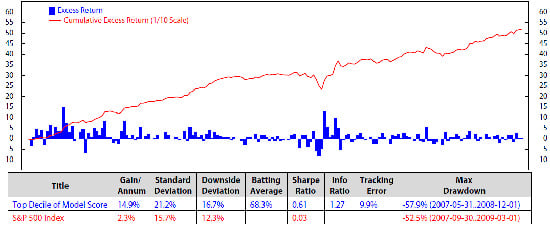
1. Introduction
In many financial problems, the states of a system can be modeled as a Markov chain in which each state depends on the previous state in a non-deterministic way. In a hidden Markov model (HMM), these states are invisible, while observations (the inputs of the model), which depend on the states, are visible. An observation at time t of an HMM has a certain probability distribution corresponding to a possible state.
Researchers have applied HMM for analyzing economic trends. HMM was used in [1] with three states to predict currency crises in six developing countries. Hassan and Nath [2] used HMM to forecast the stock price for interrelated markets. Kritzman, Page and Turkington [3] applied HMM with two states to predict regimes in market turbulence, inflation and the industrial production index. Guidolin, and Timmermann [4] used HMM with four states and multiple observations to study asset allocation decisions based on regime switching in asset returns. Ang and Bekaert [5] applied a regime shift model (an other name for HMM) for international asset allocation. Nguyen [6] used HMM with both single and multiple observations to forecast economic regimes and stock prices. Nobakht, Joseph and Loni [7] implemented HMM using multiple observation data (open, close, low, high) prices of a stock to predict its close prices. However, the momenta of a stock depends on many different factors, such as the corporate financial condition and management and the overall economy and industry conditions. These factors and corresponding stock returns vary widely over different macro regimes. In addition, long-term stock investments’ returns depend on the trends of these economic factors. Therefore, in this paper, we develop a new approach of HMM: making monthly stock selections based on their historical performances on economic regimes.
We analyze the performances of stocks’ returns on each macro regime to make stock selections instead of applying HMM directly to predict their prices. Our approach differs from [3,5] in that the authors used HMM to make asset allocations, while we build up a stock portfolio based on macro regimes. We chose four main macroeconomic variables that indeed have significant effects on stock prices: inflation, industrial production index, stock market index and market volatility. First, we use HMM to predict regimes for each economic indicator for the next month. Based on the performances of stock characteristics in the past on the similar regimes, we then assign a score and weight for each characteristic. Second, we calculate a composite score of each stock based on its features’ scores and weights. Finally, we make a selection of the 50 stocks that had the highest scores among all S&P 500 stocks to add to our portfolio and continue the stock selection process at the end of each month.
The paper is organized as follows: Section 2 gives a brief overview of the hidden Markov model. Section 3 describes our data selection and applications of HMM in the predictions of economic regimes and stock evaluations. Section 4 presents our experiment results and analyzes their performance, and Section 5 gives conclusions.
2. A Brief Introduction of the Hidden Markov Model
The hidden Markov model is a model that can capture the hidden states of observation data. An observation at time t of an HMM has a certain probability distribution corresponding to a possible state. The mathematical foundations of HMM were developed by Baum and Petrie in 1966 [8]. Four years later, in 1970, Baum and his colleagues published a maximization method in which the parameters of HMM are calibrated using a single observation [9]. In 1983, Levinson, Rabiner and Sondhi [10] introduced a maximum likelihood estimation method for HMM with multiple observation training, assuming that all of the observations are independent. In 2000, Li, Parizeau and Plamondon [11] presented an HMM training for multiple observations without the assumption of the independence of observations.
The basic elements of a hidden Markov model are:
- Length of observation data, T
- Number of states, N
- Number of symbols per state, M
- Observation sequence,
- Hidden state sequence,
- Possible values of each state,
- Possible symbols per state,
- Transition matrix, , where
- Vector of initial probability of being in state (regime) at time , , where
- Observation probability matrix, , where and
In summary, the parameters of an HMM are the matrices A and B and the vector p. For convenience, we use a compact notation for the parameters, given by:
If the observation probability assumes the Gaussian distribution, then , where and are the mean and variance of the distribution corresponding to the state , respectively, and is a Gaussian density function. Then, the parameters of HMM are:
where μ and σ are vectors of the means and variances of the Gaussian distributions, respectively.
We will now introduce three main problems of a hidden Markov model that must be solved:
- Given the observation data and the model parameters , how do we compute the probabilities of the observations, ?
- Given the observation data and the model parameters , how do we choose the best corresponding state sequence ?
- Given the observation data , how do we calibrate HMM parameters, , to maximize ?
In this section, we introduce algorithms known as the forward algorithm, backward algorithm, Viterbi algorithm and Baum–Welch algorithm. Either forward or backward algorithms [12,13] can be used for Problem (i), while both of these algorithms are used in the Baum–Welch algorithm [14] for Problem (iii). The Viterbi algorithm ([15,16]) solves Problem (ii). These following algorithms are written based on [12,13,14,15,16,17].
2.1. Forward Algorithm
We define the joint probability function as , then calculate recursively. The probability of observation is just the sum of the .
| The forward algorithm. |
|
2.2. Backward Algorithm
Similar to the forward algorithm, we define the conditional probability , for . Then, we have the following recursive backward algorithm.
2.3. The Viterbi Algorithm
The Viterbi method that was suggested in [15,16] is used to solve the second problem of HMM. The goal here is to find the best sequence of states when is given. While Problem 1 has exactly one solution, this problem has many possible solutions. Among these solutions, we need to find the one with the “best fit”. We define:
By induction, we have:
| The backward algorithm. |
|
Using , we can solve for the most likely state , at time t, as:
Thus, the Viterbi algorithm is given below.
| The Viterbi algorithm. |
|
The forward algorithm, backward algorithm and Viterbi algorithm can be used for multiple observation data with minor changes. We present the most important algorithm, the Baum–Welch algorithm for single observations.
2.4. Baum–Welch Algorithm
We turn to the solution for the third problem, which is the most difficult problem of HMM, where we have to find the parameters to maximize the probability of observation data . Unfortunately, given observation data, there is no way to find the global maximum of . However, we can choose the parameters, such that is locally maximized using the Baum–Welch iterative method [14], which used the maximum likelihood estimator (MLE) to train the model parameters. In order to describe the procedure, we defined , the probability of being in state at time t, as:
The probability of being in state at time t and state at time , is defined as:
Clearly,
| The Baum–Welch algorithm |
|
If the observation probability , defined in Section 2, is Gaussian, we will use the following formula to update the model parameter,
3. Describe the Model and Data
The hidden Markov model is well known for detecting or predicting regimes; therefore, it was used to detect economic trends [1,3,4,5,6] or to predict index prices [2,6,7]. In this paper, we discover a new application of HMM: making monthly stock selections based on economic indicators’ regimes. In this section, we discuss how to use HMM to predict economic regimes and stock selections in terms of the preference of the S&P 500 index. We will present the process by describing the data that were used and the constructions of using HMM for stock selections. First, we will describe preferred data for the model.
3.1. Data Selections
After analyzing the performances of the benchmark market index (S&P 500) on two defined regimes of different economic indicators, we found that the S&P 500 performs significantly different across different states of four macroeconomic variables: inflation (consumer price index (CPI)), industrial production index (INDPRO), stock market index (S&P 500) and market volatility (VIX), a measure of market expectations of near-term volatility conveyed by S&P 500 stock index option prices. Thus, we chose these four variables as the four macroeconomic indicators for our model. These are the definitions of the variables:
- Inflations: we use the 12-month changes (%) in CPI where CPI is the consumer price indexes, the monthly changes in the prices paid by urban consumers for a representative basket of goods and services of all items (not seasonally adjusted). Data source: Bureau of Labor Statistics, U.S. Department of Labor (http://www.bls.gov/cpi/).
- Industrial production index, INDPRO: we use the monthly changes of real output for all facilities located in the United States manufacturing, mining and electric and gas utilities (excluding those in U.S. territories). Data source: Board of Governors of the Federal Reserve System (http://www.federalreserve.gov/).
- Stock market index: we use one-month changes of the S&P 500 index where the Standard & Poor’s 500 (S&P 500) is an American stock market index based on the market capitalizations of 500 large companies having common stock listed on the New York stock exchange (NYSE) or the National Association of Securities Dealers Automated Quotations (NASDAQ). Data source: Yahoo Finance (http://finance.yahoo.com/).
- Market volatility: we use the Chicago Board Options Exchange Market (CBOE) Volatility Index, VIX. Data source: Chicago Board of Options Exchange (http://www.cboe.com/).
We next elect five stock return factors from two groups: the valuation group and the growth group. We collect stock characteristic (factor) data for all stocks in the S&P 500 universe from January 1990 to December 2014. Stock price data were provided by Mergent, and stock fundamental data (e.g., earnings, sales) were provided by Compustat. In the stock valuation group, we named the three following factors:
- Earnings/price (E/P) is calculated by the earning accumulation over the trailing twelve months of the stock divided by weekend price. A higher number indicates greater value for each unit of earnings, which tends to drive higher stock returns.
- The free cash flow/enterprise value is calculated by the cash flow minus cash dividends minus capital expenditures divided by market value of equity plus debt. A higher number is better.
- The sales/enterprise value is calculated by the sales accumulation over the trailing twelve months of the stock divided by the market value of equity plus debt (enterprise value). A higher sales/enterprise value signifies that each unit of a stock’s value is used to generate more sales, which normally leads to higher stock returns.
All valuation measures are presented as yields (e.g., earning/price instead of the traditional form price/earning) for more accurate, comparative purposes. Raw fundamental data can provide values close or equal to zero, which heavily skew traditional valuation metrics. Inverting the traditional valuation calculation (i.e., creating valuation yield measures) mitigates this problem and also allows for direct comparison to non-equity investments (e.g., bond yields). Furthermore, valuation yields better accommodate the display of distributions containing negative numbers (more robust summary statistics).
In the stock growth group, we choose the two factors below:
- Long-term earning per share (L-T EPS) growth: projected long-term growth rate of earning per share based on a five-year moving regression trend line. A high earnings growth rate normally leads to higher future returns.
- Long-term sales (L-T sales) growth: projected long-term growth rate of sales based on a five-year moving regression trend line. A high sales growth rate normally leads to higher future returns.
We define stock characteristic reward (factor performance) as the returns of the strategy of long top 50 stocks (ranked by the characteristic) in the S&P 500.
3.2. Description of Model
Using these above variables, our stock selections were divided into two steps. The first step is to find regimes of macro variables, and the second step is to make stock selection. Among these four macroeconomic indicators, CPI and INDPRO are monthly data, while VIX and the S&P 500 index are daily data. Thus, we use monthly frequency to take advantage of fresh data. Furthermore, using monthly data will give a moderate rotation rate, the average of time (months) a stock stays in the portfolio, for our composite portfolio.
First, we calibrate HMM’s parameters, , using the Baum–Welch algorithm, (in Section 2.4), and one of the four macroeconomic variables above. We then use the obtained parameters to predict the corresponding hidden regimes of each economic indicator using the Viterbi algorithm (in Section 2.3). We use monthly historical data of the variables from January 1990 to December 2014 for the first step. In the second step, we make monthly selections starting from December 1999 to December 2014. In this step, we choose fifty stocks based on their characteristic (factor) performances. Each month, after predicting economic regimes of the four macroeconomic variables (CPI, INDPRO, S&P 500, VIX) for a period from the target month back to the past (January 1990) in Step 1, we look back in history for periods with similar regimes as those of the next month and examine the five stock characteristics (defined in Section 3.1) to determine how well the stock factors performed in these periods. We then give score and weight to each factor and form a composite score for each stock of the S&P 500. Finally, we select a portfolio of the best 50 stocks (top decile) and compare the performances of the portfolio over time with the benchmark index (S&P 500). We continue the stock evaluation process by updating the parameters of HMM and adding the value of the most recent month for the macro variables, to make a new prediction. We will present more details about the processes in the next sections.
4. Implementations and Results
In this section, we will go into further detail in explaining the two steps of stock selection presented in Section 3.2, as well as presenting the results corresponding to their implementation.
4.1. Regimes of Macro Variables
Our first approach to stock selection is using HMM to find regimes for four economic macro variables: inflations, industrial production index, stock market index and market volatility. We focus on finding only two opposite states of these four economic indicators to keep the model simple while maintaining the predictive power as reasonable. In addition, most macro variables often experience two opposite states: bull/bear for the stock index, S&P 500, inflation/deflation for inflation, CPI, low/high volatility for market volatility, VIX, and growth/recession for the industrial production index, INDPRO. Therefore, we just need two states, State 1 and State 2, for our model. We define State (or Regime) 2 as the regime corresponding to the normal distribution that has the lower ratio of mean and variance. For the stock market variable, State 1 represents the bull market, and State 2 represents the bear market. For the inflation variable, State 1 stands for inflation and State 2 stands for deflation. For the industrial production index variable, State 1 and State 2 interpret growth and recession, respectably. For the market volatility State 1 represents low volatility, and State 2 represents high volatility.
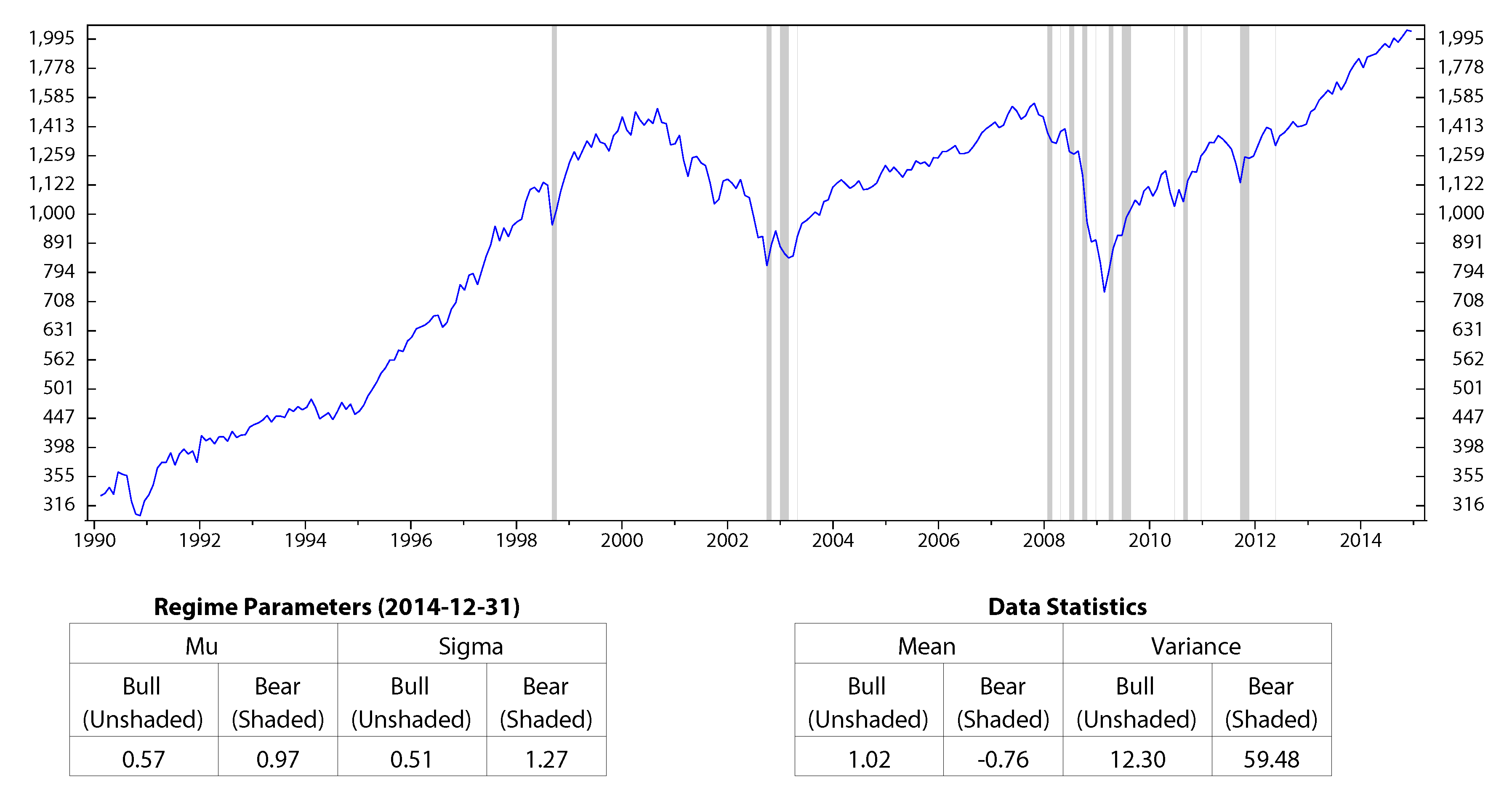
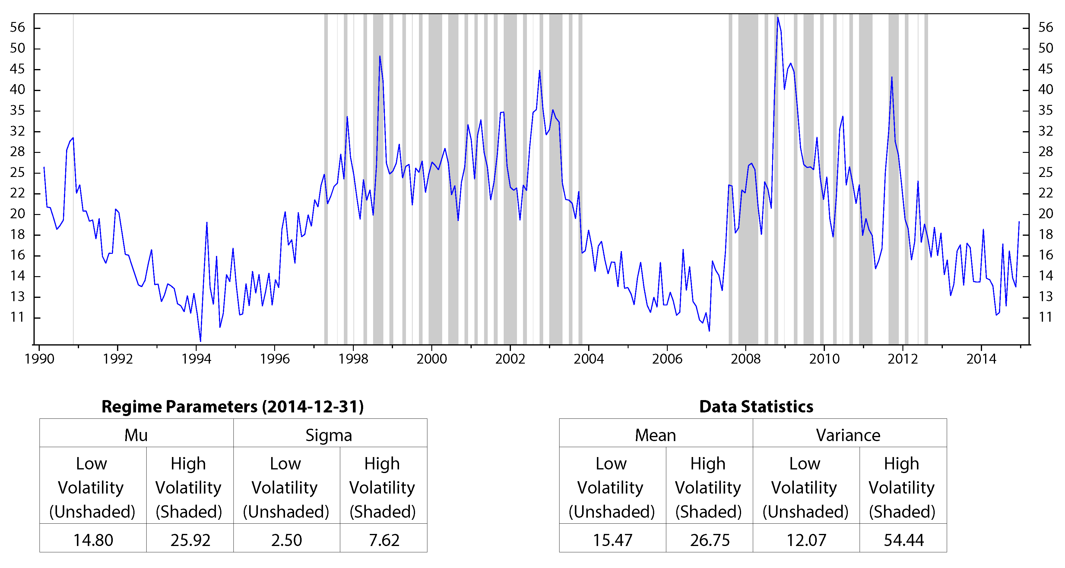
We use historical data of each variable and record monthly from January 1990 to December 2014 to calibrate HMM parameters and to find the corresponding regimes. The results are shown in Figure 1 to Figure 4. On the figures, the unshaded areas represent State 1, and the shaded areas represent State 2. Under each of these figures are two tables: in one table, we report the calibrated parameters of HMM. In the other table, we summarize the mean and variance of each macro variable on the corresponding regime. In all four figures, the performance of the economic indicators on each regime (in terms of center and spread) is consistent with the definition of regimes. Figure 1 and Figure 3 show the regimes of inflation and the stock market index, respectively. The inflation rate, CPI, has a slightly higher mean during the deflations; however, it also has higher variance compared to those during the inflations. The stock market index, S&P 500, has a negative average return and high volatilities during the bear market, while it performs well in the bull market. Figure 2 shows the regimes of the industrial production index, INDPRO. The INDPRO has a lower mean and higher variance of growth rate during recessions than those during the growths. Figure 4 shows the regimes of the market volatility, VIX. We find that VIX is more stable during high volatilities than during low volatilities.
The results above indicate that using different economic indicator HMM gives different predictions for economic regimes. Furthermore, it is clear from the four Figure 1 to Figure 4 that each of the macro variables was in State 2 during the economic crisis period from 2008 to 2010. We have the conclusion that HMM can predict economic crisis by using a proper economic indicator.
Figure 1.
Regimes of inflation, CPI; monthly data from January 1990 to December 2014 (log scale).

Figure 2.
Regimes of the industrial production index, INDPRO; monthly data from January 1990 to December 2014 (log scale).
Figure 2.
Regimes of the industrial production index, INDPRO; monthly data from January 1990 to December 2014 (log scale).

Figure 3.
Regimes of the stock market index, S&P 500; monthly data from January 1990 to December 2014 (log scale).
Figure 3.
Regimes of the stock market index, S&P 500; monthly data from January 1990 to December 2014 (log scale).

Figure 4.
Regimes of market volatility, VIX; monthly data from January 1990 to December 2014 (log scale).
Figure 4.
Regimes of market volatility, VIX; monthly data from January 1990 to December 2014 (log scale).

4.2. Stock Selection
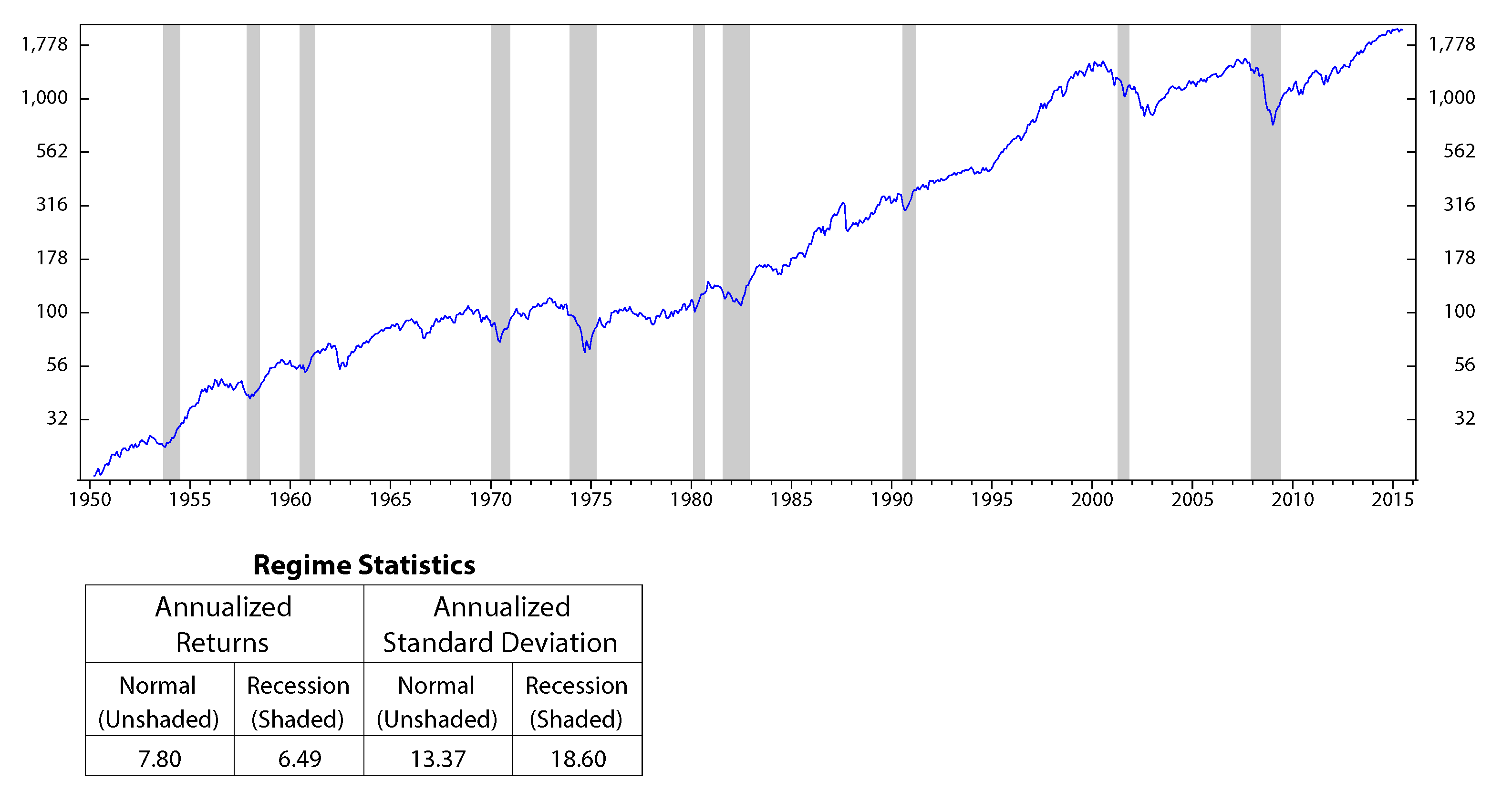
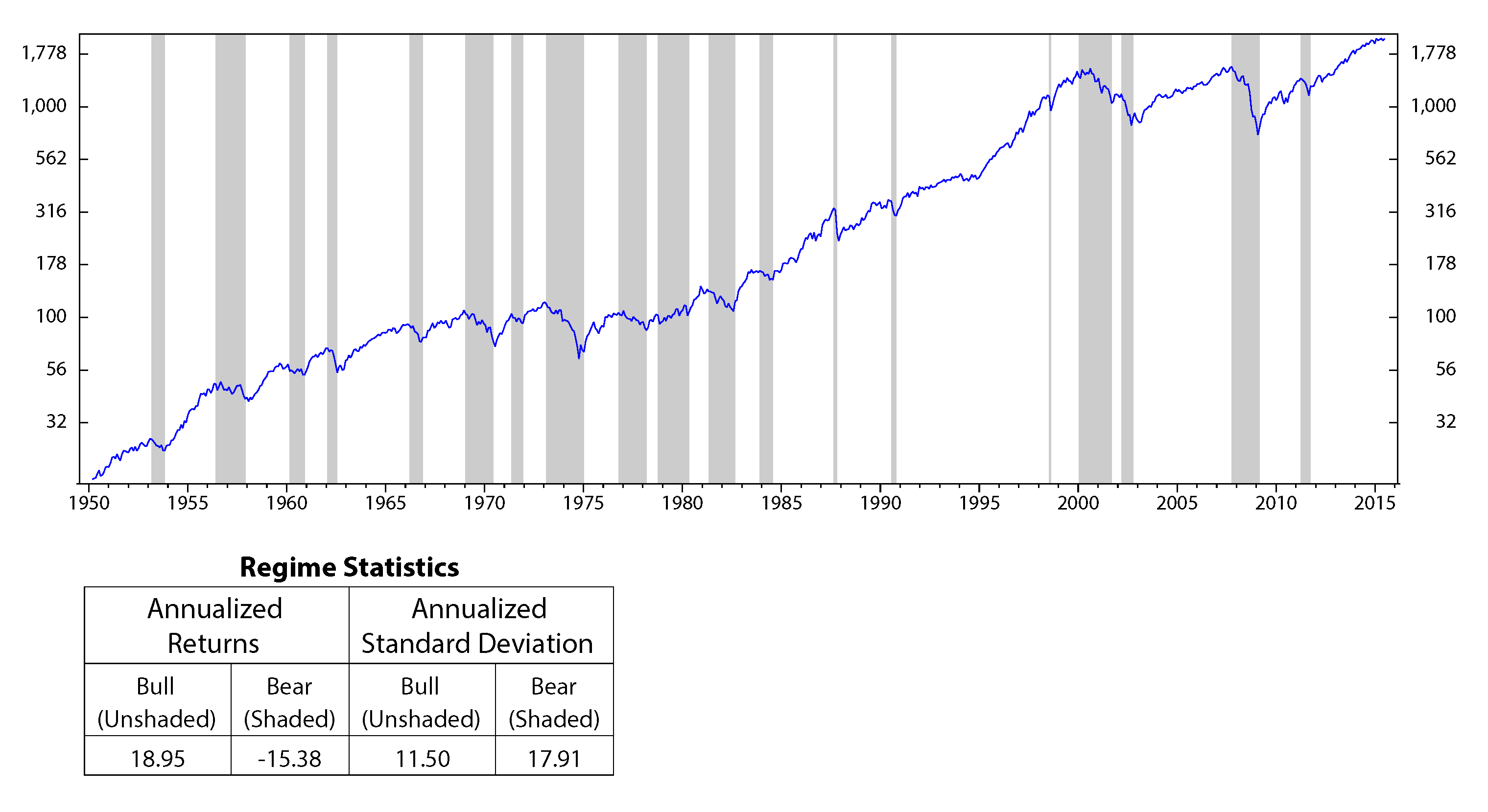
The motivation of the paper originated from observations that the stock market performs significantly different across different regimes (Figure 12 to Figure 14, in the Appendix). Our question is: can we use the performances of stocks in the past to predict their future performances? An index seems to have similar behaviors on the same economic regimes. Thus, it is reasonable to analyze stock characteristics (or stock factors) on a similar environment in the past to forecast its future outcomes. Based on this motivation, in this section, we discuss how to use HMM to make stock selections.
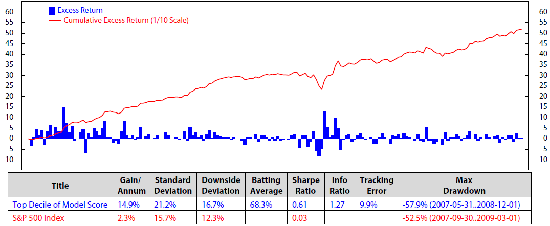
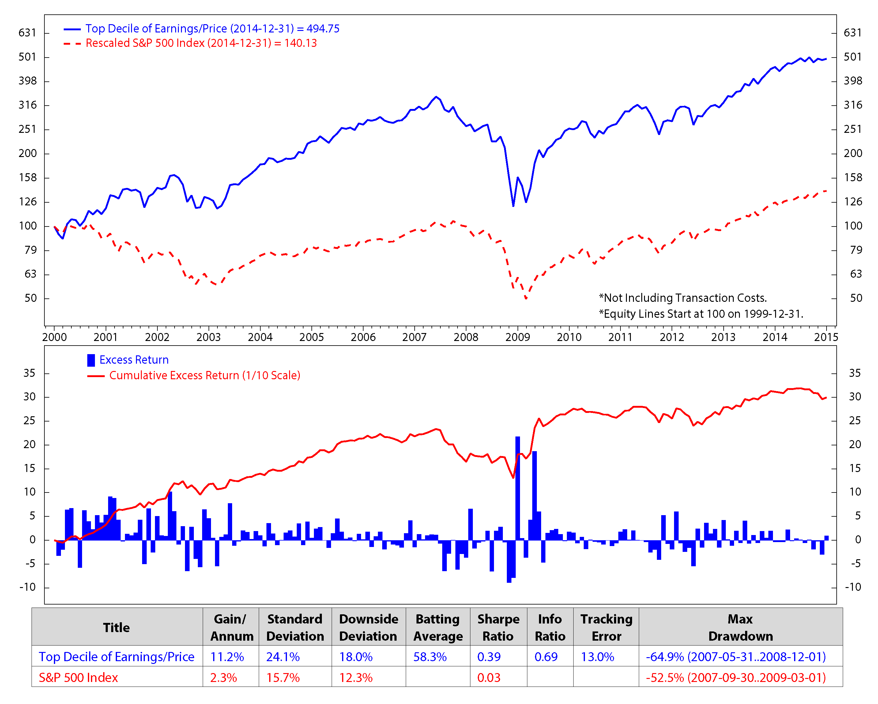
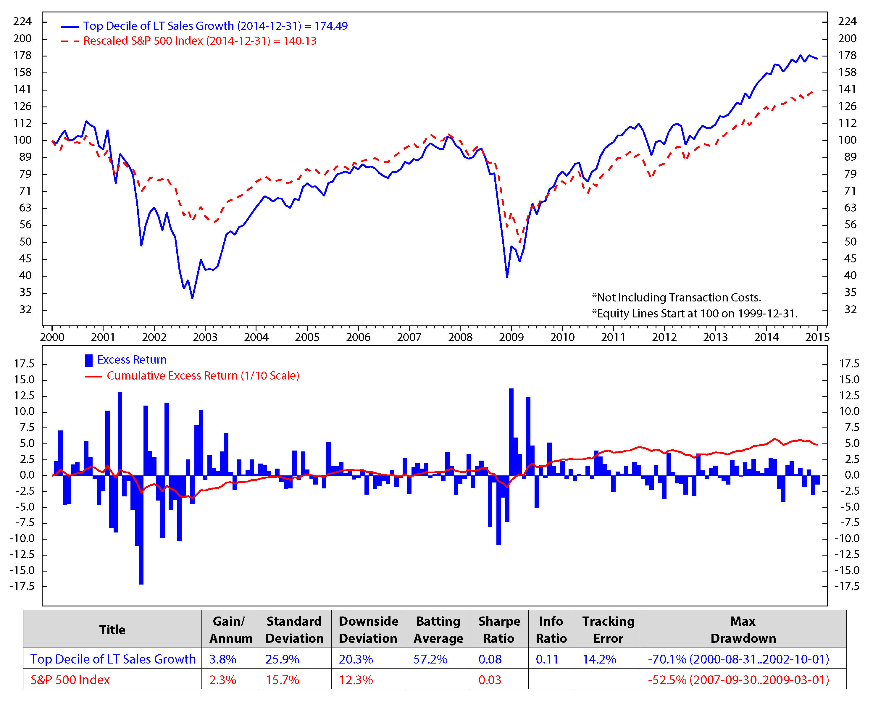
We investigate the stock factors that were affected the most by the macro regimes and use these factors to rank stocks in S&P 500. Each month, we select 50 stocks from the S&P 500 universe based on the stock ranking to add into our portfolio. The process is presented as follow. At the end of each month, we first calibrate HMM’s parameters using monthly data of each of the four macroeconomic variables: inflation, industrial production index, market index and market volatility. We then find the regimes of each variable during the time period and predict the upcoming regimes. After predicting the regimes of the four variables in the next month, we look back at historical data (twenty years) and find similar performances of these four variables. For example, if the predicted regimes for the next month of inflation, industrial production index, market index and market volatility are 1, 2, 2, 1, respectively, we will look from recent time back to twenty years in the past to find the months that these four variables had the same regimes 1, 2, 2, 1. We then check the performance of each stock factor (defined in Section 3.1: E/P, free cash flow/enterprise value, sales/enterprise value, long-term earnings per share growth and long-term sales growth). We rank each stock factor from one to five based on its performance, then assign its weight equal to the factor rank divided by the sum of all of the possible ranks (which is the sum of 1, 2, 3, 4, 5). The composite score for each stock is calculated by the summation of products of its factor ranks with the corresponding factor weights. The final composite scores were scaled to have the range from one to 100. We select 50 stocks with the highest composite score for our portfolio. We sell ones that are not in the election list while buying the newly-entered ones. Our calculation shows that once a stocks is added to our portfolio, it stays for about three months. Figure 5 to Figure 9 show the monthly performances of the stock factors of the 50 selected stocks. Each of the figures consists of two graphs. The graph on the top compares the consummation of our portfolio’s factor versus the S&P 500 returns from December 1999 to December 2014. The graph on the bottom presents the excess return and the accumulated return of the factors of our 50 chosen stocks. We scale the stock prices so that the price at the beginning of the stock electing process (December 1999) could be $100.00. At the bottom of each figure is a table that summaries the performances. We calculate the annual gain (gain/annum), standard deviation, downside deviation, batting average, Sharpe ratio, information ratio (info ratio), tracking error and maximum draw down of the data. The batting average is a statistical measure used to measure an investment model’s ability to meet or beat an index. The batting average is calculated by dividing the number of days (or months, quarters, etc.) in which the model beats or matches the index by the total number of days (or months, quarters, etc.) in the period of question and multiplying that factor by 100. In this paper, the batting average is the percent of time the portfolio returns meet/exceed the S&P 500 index returns. The tracking error measures the consistency of excess returns. It is created by taking the difference between the model return and the benchmark return every month or quarter and then calculating how volatile that difference is. Tracking error is also useful in determining just how “active” a model’s strategy is. The lower the tracking error, the closer the model follows the benchmark. The higher the tracking error, the more the model deviates from the benchmark. The Sharpe ratio (also known as the Sharpe index, the Sharpe measure and the reward-to-variability ratio) is a way to examine the performance of an investment by adjusting for its risk. The ratio measures the excess return (or risk premium) per unit of deviation in an investment asset or a trading strategy, typically referred to as risk (and is a deviation risk measure). In this paper, the Sharpe ratio is calculated by taking the ratio of excess returns (h1versus. S&P 500 index) and its standard deviation.
Figure 5.
Comparison of earnings/price and the S&P 500; monthly data from December 1999 to December 2014 (log scale).
Figure 5.
Comparison of earnings/price and the S&P 500; monthly data from December 1999 to December 2014 (log scale).

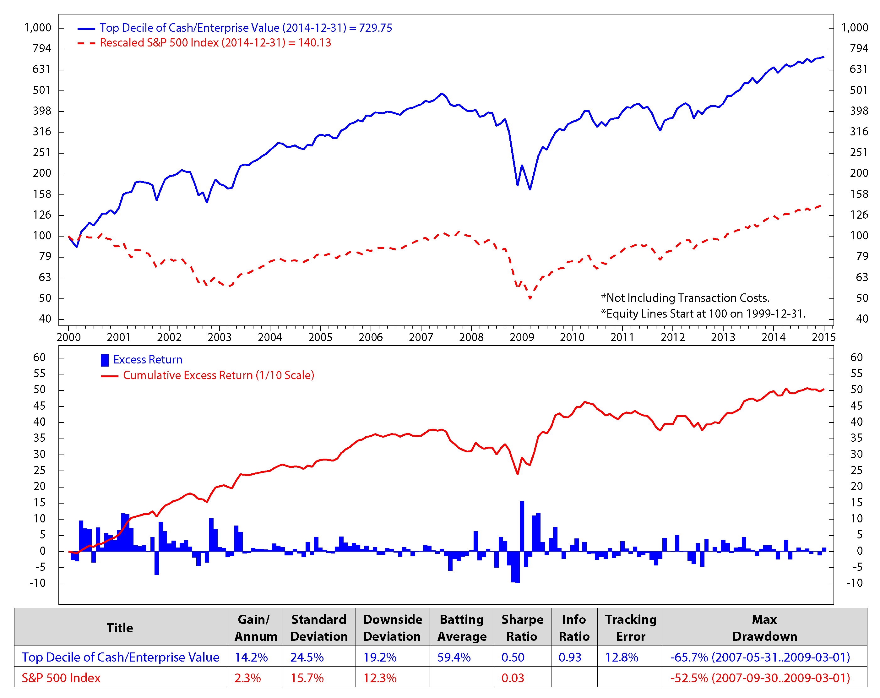
Figure 6.
Comparison of free cash flow/enterprise value and the S&P 500; monthly data from December 1999 to December 2014 (log scale).
Figure 6.
Comparison of free cash flow/enterprise value and the S&P 500; monthly data from December 1999 to December 2014 (log scale).

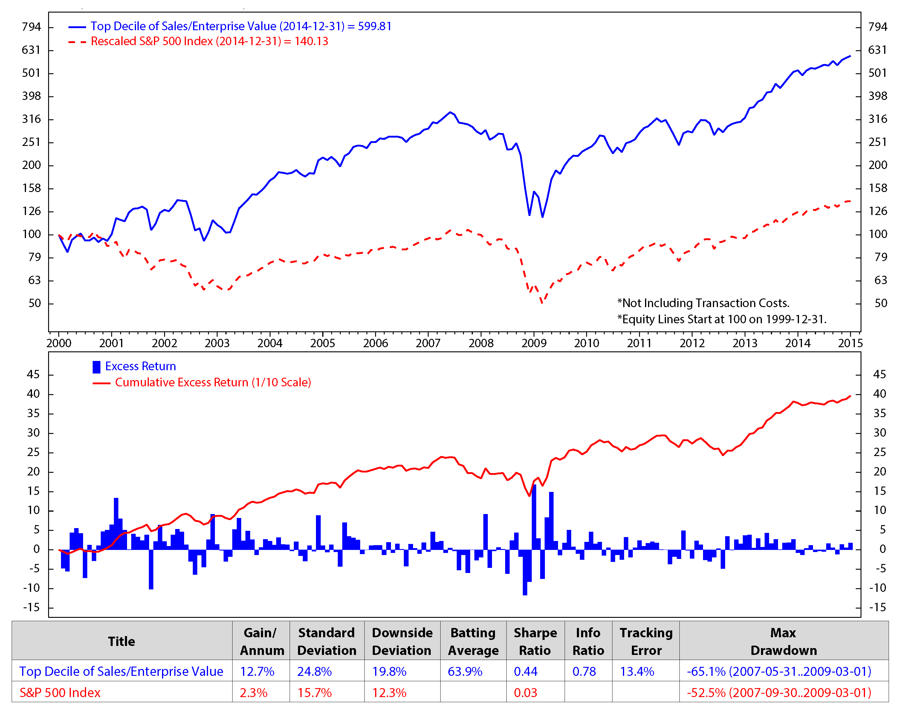
Figure 7.
Comparison of sales/enterprise value and the S&P 500; monthly data from December 1999 to December 2014 (log scale).
Figure 7.
Comparison of sales/enterprise value and the S&P 500; monthly data from December 1999 to December 2014 (log scale).

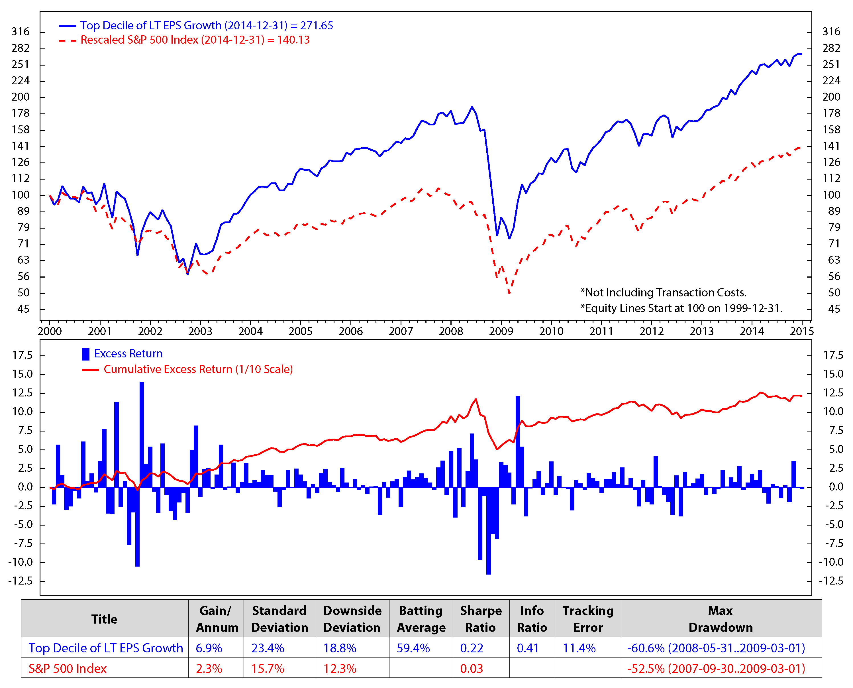
Figure 8.
Comparison of top decile of long-term earning per share (L-T EPS) growth vs. the S&P 500; monthly data from December 1999 to December 2014 (log scale).
Figure 8.
Comparison of top decile of long-term earning per share (L-T EPS) growth vs. the S&P 500; monthly data from December 1999 to December 2014 (log scale).

We make an assumption that at the end of each month, we would sell all of the stocks in our portfolio that are not on the list of the new 50 elected stocks and buy the new named stocks for the next month without transaction fees. The transaction cost is expected to be minimal in our model, because, based on our portfolio performances, the holding period of the portfolio constituents is about three months. The figures show clearly that the stock returns and the valuation factors dropped significantly during the economic crisis starting from the third quarter of 2007 to the first quarter of 2009. The five factors of the preferred stocks perform better than the S&P 500 in terms of the accumulated return.
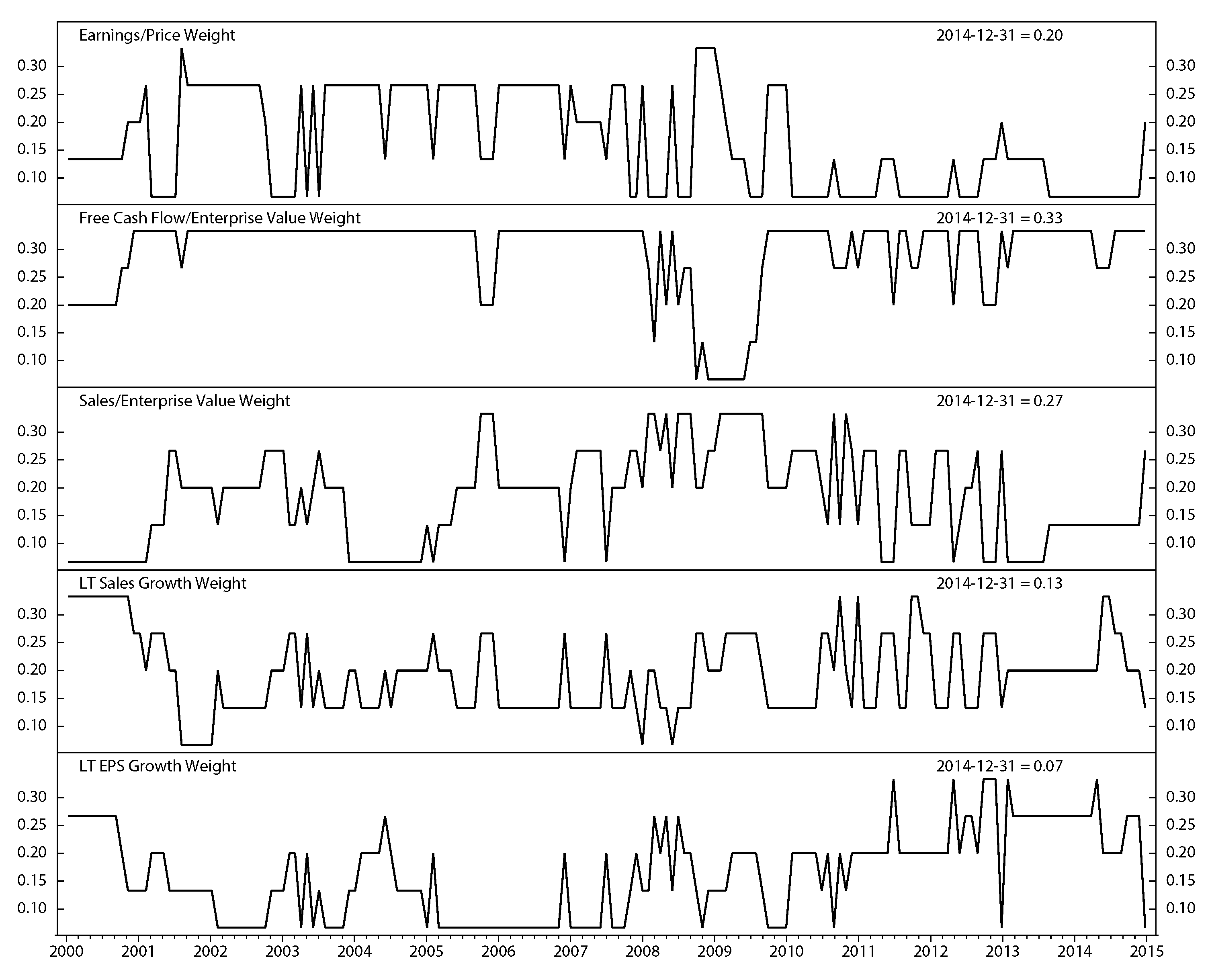
Stock factor returns are significantly different in each economic regime. Thus, we assign the weight for each factor based on its execution. Figure 10 represents the weights of each stock factor monthly from December 1999 to December 2014.
Figure 9.
Comparison of top decile of LT sales growth vs. the S&P 500; monthly data from December 1999 to December 2014 (Log Scale).
Figure 9.
Comparison of top decile of LT sales growth vs. the S&P 500; monthly data from December 1999 to December 2014 (Log Scale).

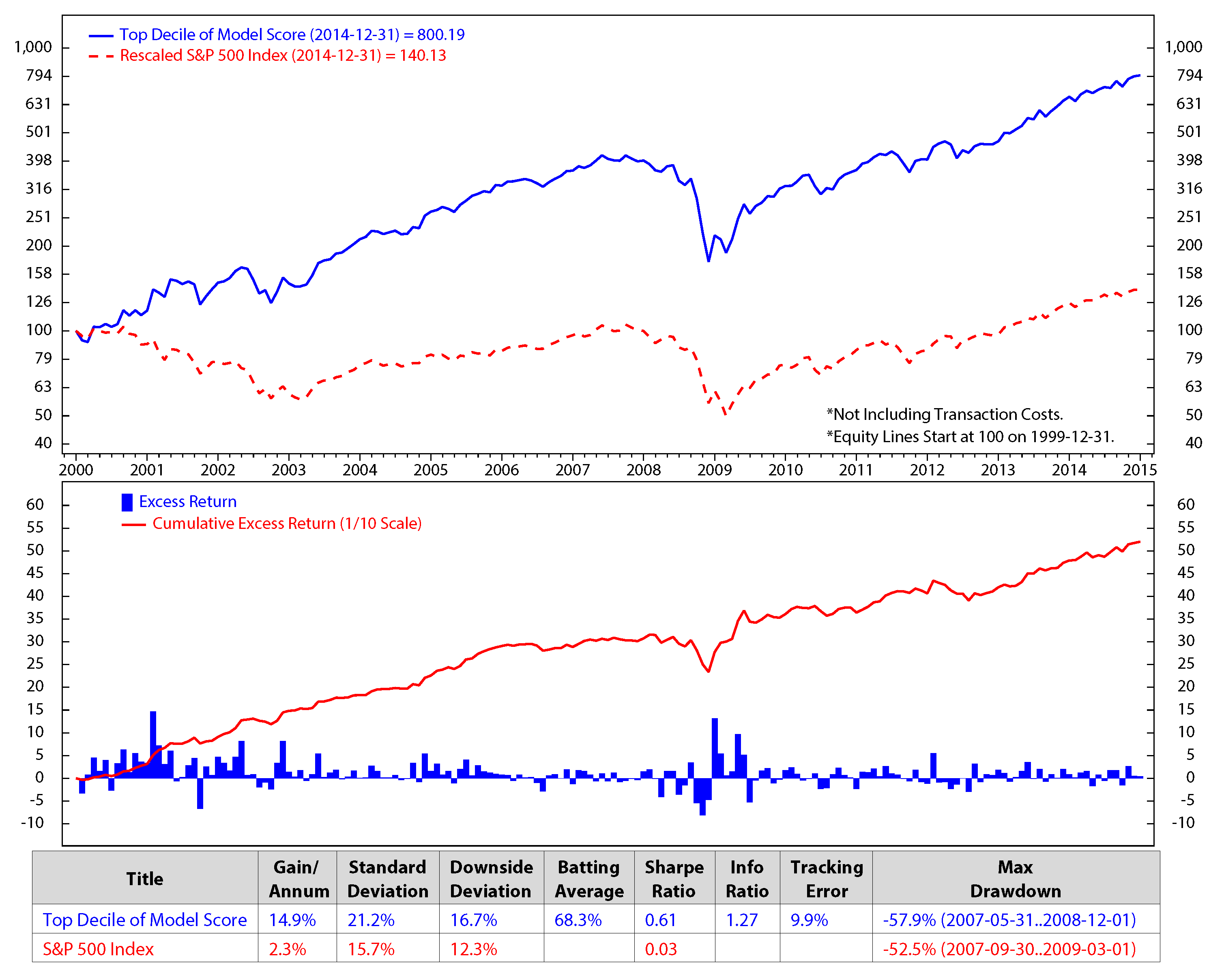
Figure 11 shows the accumulated returns of our stock selection portfolios versus that the of the S&P 500 returns. Our stock portfolio has higher returns than the S&P 500. Based on our model, with an initial investment of $100, in the 15 years from December 1999 through December 2014, our portfolio had an average gain per annum of 14.9% versus 2.3% for the S&P 500. The gains were calculated without transaction fees. Our portfolio returns were the result of monthly trading; on the other hand, the earnings of the S&P 500 were estimated by buy and hold for the long term, that is fifteen years. Our portfolio performance is also better than the performance of any single factor strategy. Compared to the best factor strategy of long top 50 stocks of the free cash flow/enterprise value during the period (Figure 6), our portfolio shows an excess return of 0.7% (i.e., 14.9% vs. 14.2%). Most importantly, our portfolio also has lower risk, thanks to the diversification of risk across various factor strategies. As a result, its Sharpe ratio (i.e., return/risk) is higher than that of the free cash flow/enterprise value factor strategy (0.61 vs. 0.5).
Figure 10.
Weight of five stock factors; monthly data from December 1999 to December 2014.

Figure 11.
Comparison of stock selected portfolio using HMM and the S&P 500 from December 1999 to December 2014.
Figure 11.
Comparison of stock selected portfolio using HMM and the S&P 500 from December 1999 to December 2014.

5. Conclusions
Inflation, the industrial production index, the market index and the market volatility have significant impacts on the stock market. Stock performances differ during regimes of those macroeconomic indicators. Each month, we used HMM to predict the regimes for all of these variables for the upcoming month and tracked the historical data to find similar macro environments. After finding the similar periods, we examined five stock characteristics to determine their scores and weights based on their rewarded returns. We assigned the composite score for each stock in the S&P 500 universe based on the scores and weights of its factors. Finally, we chose the 50 top ranked stocks and hold for at least a month. Our backtests showed that using HMM for stock selections made significant portfolio returns compared to those of the S&P 500 universe.
Acknowledgments
The authors thank Brian Sanborn, Chartered Financial Analyst (CFA) charterholder, a global quantitative equity strategist and his quantitative team at Ned Davis Research Group, for many useful discussions and for the data used in this work.
Author Contributions
Nguyet Nguyen and Dung Nguyen contributed equally to the conception, findings and writing of the paper.
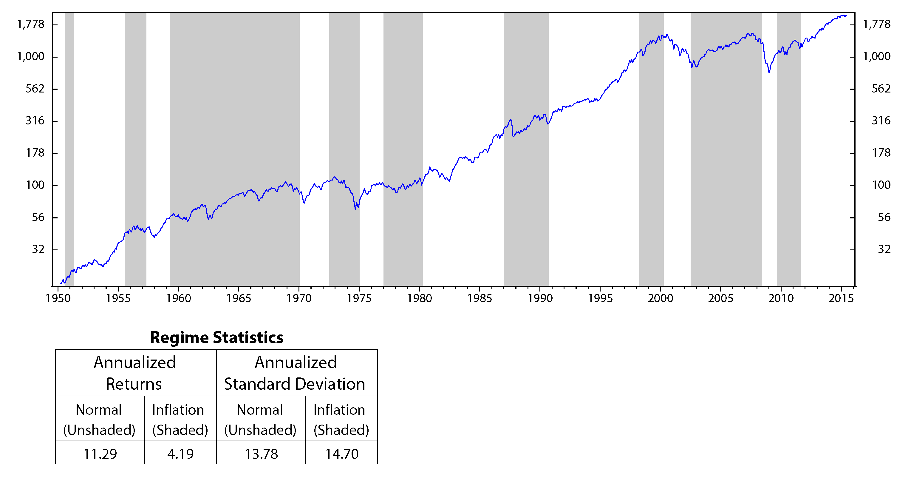
A. Stock Performance on Different Economic Regimes
Figure 12.
S&P 500 performances versus the industrial production index’s regimes; monthly data January 1950 to July 2015 (log scale).
Figure 12.
S&P 500 performances versus the industrial production index’s regimes; monthly data January 1950 to July 2015 (log scale).

Figure 13.
S&P 500 performances versus the market volatility’s regimes; monthly data January 1950 to July 2015 (log scale).
Figure 13.
S&P 500 performances versus the market volatility’s regimes; monthly data January 1950 to July 2015 (log scale).

Figure 14.
S&P 500 performances versus the inflation’s regimes; monthly data January 1950 to July 2015 (log scale).
Figure 14.
S&P 500 performances versus the inflation’s regimes; monthly data January 1950 to July 2015 (log scale).

Conflicts of Interest
The authors declare no conflict of interest.
References
- C. Chen. “How well can we predict currency crises? ” In Evidence from a three-regime Markov-Switching model. Davis, CA, USA: Department of Economics, UC Davis, 2005. [Google Scholar]
- M.R. Hassan, and B. Nath. “Stock Market Forecasting Using Hidden Markov Models: A New approach.” In Proceeding of the IEEE fifth International Conference on Intelligent Systems Design and Applications, Wroclaw, Poland, 8–10 September 2005.
- M. Kritzman, S. Page, and D. Turkington. “Regime Shifts: Implications for Dynamic Strategies.” Financ. Anal. J. 68 (2012). [Google Scholar] [CrossRef]
- M. Guidolin, and A. Timmermann. “Asset Allocation under Multivariate Regime Switching.” J. Econ. Dyn. Control 31 (2007): 3503–3544. [Google Scholar] [CrossRef]
- A. Ang, and G. Bekaert. “International Asset Allocaion with Regime Shifts.” Rev. Financ. Stud. 15 (2002): 1137–1187. [Google Scholar] [CrossRef]
- N. Nguyen. “Probabilistic Methods in Estimation and Prediction of Financial Models.” In Electronic Theses. Tallahassee, FL, USA: Treatises and Dissertations, Florida State University, 2014, p. 9059. [Google Scholar]
- B. Nobakht, C.E. Joseph, and B. Loni. “Stock market analysis and prediction using hidden markov models.” In Proceeding of the 2012 Students Conference on Engineering and Systems (SCES), Allahabad, Uttar Pradesh, India, 16–18 March 2012; pp. 1–4.
- L.E. Baum, and T. Petrie. “The Annals of Mathematical Statistics.” Stat. Inference Probab. Funct. Finite State Markov Chains 37 (1966): 1554–1563. [Google Scholar]
- L.E. Baum, T. Petrie, G. Soules, and N. Weiss. “A maximization technique occurring in the statistical analysis of probabilistic functions of Markov chains.” Ann. Math. Stat. 41 (1970): 164–171. [Google Scholar] [CrossRef]
- S.E. Levinson, L.R. Rabiner, and M.M. Sondhi. “An introduction to the application of the theory of probabilistic functions of Markov process to automatic speech recognition.” Bell Syst. Techn. J. 62 (1983): 1035–1074. [Google Scholar] [CrossRef]
- X. Li, M. Parizeau, and R. Plamondon. “Training Hidden Markov Models with Multiple Observations—A Combinatorial Method.” IEEE Trans. PAMI 22 (2000): 371–377. [Google Scholar]
- L.E. Baum, and J.A. Egon. “An inequality with applications to statistical estiation for probabilistic functions of Markov process and to a model for ecnogy.” Bull. Am. Meteorol. Soc. 73 (1967): 360–363. [Google Scholar] [CrossRef]
- L.E. Baum, and G.R. Sell. “Growth functions for transformations on manifolds.” Pac. J. Math 27 (1968): 211–227. [Google Scholar] [CrossRef]
- L.R. Rabiner. “A Tutorial on Hidden Markov Models and Selected Applications in Speech Recognition.” IEEE 77 (1989): 257–286. [Google Scholar] [CrossRef]
- G.D. Forney. “The Viterbi algorithm.” IEEE 61 (1973): 268–278. [Google Scholar] [CrossRef]
- A.J. Viterbi. “Error bounds for convolutional codes and an asymptotically optimal decoding algorithm.” IEEE Trans. Informat. Theory IT-13 (1967): 260–269. [Google Scholar] [CrossRef]
- V. A. Petrushin. “Hidden Markov Models: Fundamentals and Applications.” http://www.cis.udel.edu/ lliao/cis841s06/hmmtutorialpart2.pdf (accessed on 28 October 2015).
© 2015 by the authors; licensee MDPI, Basel, Switzerland. This article is an open access article distributed under the terms and conditions of the Creative Commons Attribution license (http://creativecommons.org/licenses/by/4.0/).
Share and Cite
MDPI and ACS Style
Nguyen, N.; Nguyen, D. Hidden Markov Model for Stock Selection. Risks 2015, 3, 455-473. https://doi.org/10.3390/risks3040455
AMA Style
Nguyen N, Nguyen D. Hidden Markov Model for Stock Selection. Risks. 2015; 3(4):455-473. https://doi.org/10.3390/risks3040455
Chicago/Turabian StyleNguyen, Nguyet, and Dung Nguyen. 2015. "Hidden Markov Model for Stock Selection" Risks 3, no. 4: 455-473. https://doi.org/10.3390/risks3040455