Article

On the Joint Analysis of the Total Discounted Payments to Policyholders and Shareholders: Dividend Barrier Strategy

1
Department of Statistics and Actuarial Science, University of Hong Kong, Pokfulam, Hong Kong
2
Department of Statistics and Actuarial Science, University of Iowa, Iowa City, IA 52242, USA
*
Author to whom correspondence should be addressed.
Risks 2015, 3(4), 491-514; https://doi.org/10.3390/risks3040491
Submission received: 9 October 2015 / Accepted: 3 November 2015 / Published: 10 November 2015

Abstract

:
In the compound Poisson insurance risk model under a dividend barrier strategy, this paper aims to analyze jointly the aggregate discounted claim amounts until ruin and the total discounted dividends until ruin, which represent the insurer’s payments to its policyholders and shareholders, respectively. To this end, we introduce a Gerber–Shiu-type function, which further incorporates the higher moments of these two quantities. This not only unifies the individual study of various ruin-related quantities, but also allows for new measures concerning covariances to be calculated. The integro-differential equation satisfied by the generalized Gerber–Shiu function and the boundary condition are derived. In particular, when the claim severity is distributed as a combination of exponentials, explicit expressions for this Gerber–Shiu function in some special cases are given. Numerical examples involving the covariances between any two of (i) the aggregate discounted claims until ruin, (ii) the discounted dividend payments until ruin and (iii) the time of ruin are presented along with some interpretations.

1. Introduction

The study of the aggregate (non-discounted) claims has been a classical and important topic in collective risk theory (see, e.g., [1,2] for reviews). Exact results concerning the Laplace transform and the moments of the aggregate discounted claims have also been obtained by, e.g., [3,4,5,6,7]. Traditionally, the analysis of the aggregate claims is mostly concerned with the aggregate until a fixed time t > 0 . Recently, there has been increased interest in the aggregate claims until the ruin time of the underlying risk process (instead of a fixed time). Specifically, under the (perturbed) compound Poisson model and the phase-type renewal models, [8,9] studied the distribution of the aggregate claims until ruin without discounting; whereas [10] (Section 6), [11] (Section 4.2) and [12] (Section 5.2) analyzed the expected aggregate discounted claims until ruin. The higher moments of the aggregate discounted claims until ruin were also considered by [13] (Section 2.1) in a risk process with Markovian claims arrival (e.g., [14], Chapter XI.1), by [15] in a renewal risk model with arbitrary inter-claim times and by [16] in a dependent Sparre–Andersen risk model (e.g., [17]).
However, the aforementioned contributions in the literature mainly focused on the individual treatment of the moments and/or the distribution of the aggregate claims in various models, and little has been said about the relationship between the aggregate claim amounts and other ruin-related quantities. An exception is [16], who have recently analyzed the covariance of the aggregate discounted claims until ruin and the time of ruin (conditional on ruin occurring). In the context of a dependent Sparre–Andersen risk model where the inter-claim time and the resulting claim amount are modeled via a Farlie–Gumbel–Morgenstern copula with exponential marginals, they provided numerical illustrations showing that the above covariance could possibly take a negative value and gave some probabilistic interpretations, as well. In addition to the time of ruin, in this paper, we are also interested in the relationship of the aggregate discounted claims until ruin, particularly with the total discounted dividends paid until ruin. Note that the insurer’s surplus is drained by payments made not only to the policyholders (claims), but also to the shareholders (dividends). The dividend payouts are determined based on the overall performance of the company’s business, which is, in turn, affected by insurance claim payments. Moreover, it is worthwhile to point out that although numerous studies have been performed by various researchers on the dividend payments in different risk models, the concurrent analysis of dividends and other ruin-related quantities, such as the time of ruin and the deficit at ruin, only appears in Theorem 1 of [18] (to the best of our knowledge). The above reasoning leads us to investigate the Gerber–Shiu expected discounted penalty function [19] in which both the total discounted dividends until ruin and the aggregate discounted claims until ruin are incorporated (see Equation (3)). A merit of a this proposed approach is that it facilitates the joint analysis of the aforementioned random variables, leading to covariance measures that have never been studied before (see Section 4).
In this paper, we assume that the baseline risk process { U ( t ) } t 0 (in the absence of dividends) follows the classical compound Poisson insurance risk model. Let c > 0 be the premium rate per unit time received by the insurer, { N ( t ) } t 0 be the claims counting process, which is a Poisson process with parameter λ > 0 , and Y i be the size of the i-th claim. It is assumed that { Y i } i = 1 forms a sequence of independent and identically distributed positive continuous random variables with common probability density function p ( · ) and Laplace transform p ˜ ( · ) . In addition, { N ( t ) } t 0 and { Y i } i = 1 are assumed independent. The aggregate claims process is thus { S ( t ) } t 0 where S ( t ) = i = 1 N ( t ) Y i . With the initial surplus u = U ( 0 ) 0 , the surplus process { U ( t ) } t 0 follows the dynamics:
U ( t ) = u + c t - S ( t ) , t 0
The positive security loading condition c > λ E [ Y 1 ] is assumed to hold true. Since the concept of redistributing part of the insurer’s surplus to the shareholders was proposed by [20], the dividend strategy that has been studied the most is the barrier strategy (see, e.g., [21]). Such a strategy will be adopted in this paper, and it is known to be optimal in maximizing the expected total discounted dividends until ruin when p ( · ) is completely monotone (e.g., Theorem 3 of [22]). Under a dividend barrier strategy, whenever the surplus process reaches a fixed level b > 0 , a dividend is declared and immediately payable at rate c until the next claim occurs. The modified surplus process { U b ( t ) } t 0 can then be described by:
d U b ( t ) = { c d t d S ( t ) , U b ( t ) < b d S ( t ) , U b ( t ) = b
where the initial surplus U b ( 0 ) = u is such that 0 u b . The time of ruin of { U b ( t ) } t 0 is defined as τ b = inf { t 0 : U b ( t ) < 0 } . With D ( t ) = U ( t ) - U b ( t ) being the aggregate dividend payments until time t 0 , we define the total discounted dividends until ruin to be:
D δ ( τ b ) = 0 τ b e - δ t d D ( t ) = c 0 τ b e - δ t 1 { U b ( t ) = b } d t
where δ 0 is the force of interest and 1 A is the indicator function of the event A. In the above model, solutions to the Gerber–Shiu function and the moments of D δ ( τ b ) were derived by [23,24], respectively. The latter contribution also proposed that the shareholders should cover the deficit at ruin (now known as the “Dickson–Waters modification”), and this was later studied by [25], as well. For the further analysis of the moments of D δ ( τ b ) , interested readers are referred to [18,26] for the Lévy insurance risk process and [27,28] for a general skip-free upward stationary Markov process. We also define the aggregate discounted claim costs until ruin as:
Z δ ( τ b ) = i = 1 N ( τ b ) e - δ T i f ( Y i )
where T i is the occurrence time of the i-th claim (i.e., the i-th arrival epoch of the Poisson process { N ( t ) } t 0 ) and f ( · ) is the cost function that associates a cost to each claim. While D δ ( τ b ) represents the discounted payments made to the shareholders, the special case of Z δ ( τ b ) when f ( y ) = y corresponds to the aggregate discounted claims until ruin, which constitute the total payment to the policyholders (that can be expressed as Z δ ( τ b ) = 0 τ b e - δ t d S ( t ) ).
To provide an analytical tool to jointly study Equations (1) and (2) and other ruin-related quantities according to the above discussions, Equations (1) and (2) are now incorporated into the Gerber–Shiu function in the form of moment-based components as follows. Throughout the paper, we shall use N and N + to denote the set of non-negative integers and the set of positive integers, respectively. For n , m N , we define the Gerber–Shiu type function of our interest as, for 0 u b ,
ϕ δ 1 , δ 2 , δ 3 , n , m ( u ; b ) = ϕ δ 123 , n , m ( u ; b ) = E e - δ 1 τ b D δ 2 n ( τ b ) Z δ 3 m ( τ b ) w ( U b ( τ b - ) , | U b ( τ b ) | ) | U b ( 0 ) = u
where δ 1 0 is the Laplace transform argument with respect to the time of ruin τ b and w ( · , · ) is the penalty function that depends on the surplus prior to ruin U b ( τ b - ) and the deficit at ruin | U b ( τ b ) | . Note that we allow dividends and claims to be discounted using different interest rates δ 2 0 and δ 3 0 to account for possibly different time preferences of the shareholders and the policyholders. Moreover, the indicator function 1 { τ b < } is not needed in the above definition, because ruin occurs almost surely under a barrier strategy. The work in [15] first proposed a special case of Equation (3) when n = 0 , δ 1 = k δ 3 for some k N , and w only depends on the deficit in the context of a Sparre–Andersen risk model without dividends. The extended Gerber–Shiu function ϕ δ 123 , n , m ( u ; b ) in Equation (3) not only unifies the individual study of each variable involved, but also allows for new quantities to be evaluated. Clearly, when n = m = 0 , it reduces to the usual Gerber–Shiu function proposed by [19] (which will be denoted by ϕ δ 1 ( u ; b ) ). On the other hand, if δ 1 = 0 , n N + m = 0 and w 1 , then Equation (3) reduces to the moments of discounted dividends until ruin (e.g., [24]). Interesting new quantities that can be computed from Equation (3) include the following.
(i)
When m = 0 , then Equation (3) can be regarded as a unification of the usual Gerber–Shiu function and the dividend moments. The analysis of this special case is surprisingly simple, and the general solution can be expressed in terms of quantities available in the literature. See Section 2.3.
(ii)
When δ 1 = 0 and w 1 , Equation (3) reduces to the joint moments of D δ 2 ( τ b ) and Z δ 3 ( τ b ) , from which the covariance of D δ 2 ( τ b ) and Z δ 3 ( τ b ) can be calculated. See Section 4.
(iii)
When w 1 and n = 0 (resp. m = 0 ), the joint moments of τ b and Z δ 3 ( τ b ) (resp. D δ 2 ( τ b ) ) can be obtained by successively differentiating Equation (3) with respect to δ 1 , leading to the covariance of τ b and Z δ 3 ( τ b ) (resp. D δ 2 ( τ b ) ). See Section 4.
The remainder of the paper is organized as follows. Section 2 deals with the derivation of the integro-differential equation (IDE) in u satisfied by ϕ δ 123 , n , m ( u ; b ) along with the boundary condition. The treatment will be different depending on whether n = 0 or n N + . A general solution to ϕ δ 123 , n , 0 ( u ; b ) is given, as well. In Section 3, it is assumed that f ( y ) = y (as we are mostly interested in the aggregate discounted claims until ruin), w ( x , y ) = w ( y ) , and the distribution of each claim follows a combination of exponentials. Explicit expressions for ϕ δ 123 , n , 0 ( u ; b ) when n N , ϕ δ 123 , 0 , m ( u ; b ) when m = 1 , 2 and ϕ δ 123 , 1 , 1 ( u ; b ) are obtained. These formulas are then applied to generate numerical examples in Section 4 concerning particularly covariances involving τ b , Z δ 3 ( τ b ) and D δ 2 ( τ b ) . We also provide some explanations of the results.

2. General Results

2.1. IDE and Boundary Condition for ϕ δ 13 , m ( u ; b ) = ϕ δ 123 , 0 , m ( u ; b )

We first let n = 0 , so that the dividend component D δ 2 ( τ b ) is absent in the definition Equation (3). Such a special case is denoted by:
ϕ δ 13 , m ( u ; b ) = ϕ δ 123 , 0 , m ( u ; b ) = E e - δ 1 τ b Z δ 3 m ( τ b ) w ( U b ( τ b - ) , | U b ( τ b ) | ) | U b ( 0 ) = u
We have the following Theorem (and it is understood that any derivative ϕ δ 13 , m ( u ; b ) or, more generally, ϕ δ 123 , n , m ( u ; b ) is taken with respect to the first argument u).
Theorem 1. For m N , the Gerber–Shiu function ϕ δ 13 , m ( u ; b ) in Equation (4) satisfies the IDE:
ϕ δ 13 , m ( u ; b ) = λ + δ 1 + m δ 3 c ϕ δ 13 , m ( u ; b ) - λ c 0 u ϕ δ 13 , m ( u - y ; b ) p ( y ) d y
- λ c i = 0 m - 1 m i 0 u f m - i ( y ) ϕ δ 13 , i ( u - y ; b ) p ( y ) d y - λ c u f m ( y ) w ( u , y - u ) p ( y ) d y
for 0 u b . The boundary condition is given by:
ϕ δ 13 , m ( b ; b ) = 0
Proof. Conditioning on the occurrence time and the amount of the first claim followed by a binomial expansion, we arrive at, for 0 u b ,
ϕ δ 13 , m ( u ; b ) = 0 b - u c λ e - ( λ + δ 1 + m δ 3 ) t { 0 u + c t i = 0 m m i f m - i ( y ) ϕ δ 13 , i ( u + c t - y ; b ) p ( y ) d y + u + c t f m ( y ) w ( u + c t , y - u - c t ) p ( y ) d y } d t + b - u c λ e - ( λ + δ 1 + m δ 3 ) t { 0 b i = 0 m m i f m - i ( y ) ϕ δ 13 , i ( b - y ; b ) p ( y ) d y + b f m ( y ) w ( b , y - b ) p ( y ) d y } d t (7) = 0 b - u c λ e - ( λ + δ 1 + m δ 3 ) t γ b , m ( u + c t ) d t + b - u c λ e - ( λ + δ 1 + m δ 3 ) t γ b , m ( b ) d t
where:
γ b , m ( x ) = 0 x i = 0 m m i f m - i ( y ) ϕ δ 13 , i ( x - y ; b ) p ( y ) d y + x f m ( y ) w ( x , y - x ) p ( y ) d y
A change of variable x = u + c t in the first integral in Equation (7) along with the evaluation of the second integral gives rise to:
ϕ δ 13 , m ( u ; b ) = λ c u b e - λ + δ 1 + m δ 3 c ( x - u ) γ b , m ( x ) d x + λ λ + δ 1 + m δ 3 e - λ + δ 1 + m δ 3 c ( b - u ) γ b , m ( b )
Differentiation with respect to u leads to:
ϕ δ 13 , m ( u ; b ) = λ + δ 1 + m δ 3 c ϕ δ 13 , m ( u ; b ) - λ c γ b , m ( u )
Applying Equation (8) and separating the term i = m in the summation proves Equation (5). Finally, putting u = b in Equation (9) yields:
ϕ δ 13 , m ( b ; b ) = λ λ + δ 1 + m δ 3 γ b , m ( b )
from which the comparison with Equation (10) at u = b results in the boundary condition Equation (6). ☐
It is instructive to note that the IDE Equation (5) satisfied by ϕ δ 13 , m ( u ; b ) needs to be solved recursively in m. This is because the non-homogeneous part of Equation (5) involves the lower moments ϕ δ 13 , i ( u ; b ) for i = 0 , 1 , , m - 1 (and therefore, the starting point is the classical Gerber–Shiu function ϕ δ 1 ( u ; b ) = ϕ δ 13 , 0 ( u ; b ) ). However, it does not appear to be an easy task to obtain a general solution of ϕ δ 13 , m ( u ; b ) for m N + when the claim distribution is arbitrary, as the non-homogeneous part of the IDE depends on the barrier level b. This is in contrast to ϕ δ 1 ( u ; b ) (i.e., the case m = 0 ) for which the non-homogeneous part of the IDE does not depend on b, and therefore, the barrier-free Gerber–Shiu function ϕ δ 1 ( u ; ) can be treated as a particular solution (see [23], Section 3). In Section 3.2 and Section 3.3, we shall demonstrate how to obtain ϕ δ 13 , 1 ( u ; b ) and ϕ δ 13 , 2 ( u ; b ) when each claim is distributed as a combination of exponentials.

2.2. IDE and Boundary Condition for ϕ δ 123 , n , m ( u ; b ) When n N +

Now, we consider ϕ δ 123 , n , m ( u ; b ) in Equation (3) for n N + . For notational convenience, we define δ 123 ( n , m ) = δ 1 + n δ 2 + m δ 3 . The IDE and boundary condition satisfied by ϕ δ 123 , n , m ( u ; b ) are given in the following Theorem.
Theorem 2. For n N + and m N , the Gerber–Shiu function ϕ δ 123 , n , m ( u ; b ) in Equation (3) satisfies the IDE:
ϕ δ 123 , n , m ( u ; b ) = λ + δ 123 ( n , m ) c ϕ δ 123 , n , m ( u ; b ) - λ c 0 u ϕ δ 123 , n , m ( u - y ; b ) p ( y ) d y (12) - λ c i = 0 m - 1 m i 0 u f m - i ( y ) ϕ δ 123 , n , i ( u - y ; b ) p ( y ) d y
for 0 u b . The boundary condition is given by:
ϕ δ 123 , n , m ( b ; b ) = n ϕ δ 123 , n - 1 , m ( b ; b )
Proof. Similar to the proof of Theorem 1, we consider the event of the first claim. Note that if the first claim causes ruin before the process reaches the barrier b, then no dividend is payable before ruin (i.e., D δ 2 ( τ b ) = 0 ). With n N + , such an event contributes nothing to the Gerber–Shiu function. In addition, if the process reaches b before the first claim and the first claim does not result in ruin, then we need to apply separate binomial expansions to dividends and claims. Consolidating the above observations, one finds, for 0 u b ,
ϕ δ 123 , n , m ( u ; b ) = 0 b - u c λ e - ( λ + δ 123 ( n , m ) ) t 0 u + c t i = 0 m m i f m - i ( y ) ϕ δ 123 , n , i ( u + c t - y ; b ) p ( y ) d y d t + b - u c λ e - ( λ + δ 123 ( n , m ) ) t { b c s ¯ t - b - u c ¯ | δ 2 n f m ( y ) w ( b , y - b ) p ( y ) d y + 0 b j = 0 n n j c s ¯ t - b - u c ¯ | δ 2 n - j i = 0 m m i f m - i ( y ) ϕ δ 123 , j , i ( b - y ; b ) p ( y ) d y } d t = λ c u b e - λ + δ 123 ( n , m ) c ( x - u ) 0 x i = 0 m m i f m - i ( y ) ϕ δ 123 , n , i ( x - y ; b ) p ( y ) d y d x + 0 λ e - ( λ + δ 123 ( n , m ) ) t + b - u c { b c s ¯ t ¯ | δ 2 n f m ( y ) w ( b , y - b ) p ( y ) d y (14) + 0 b j = 0 n n j c s ¯ t ¯ | δ 2 n - j i = 0 m m i f m - i ( y ) ϕ δ 123 , j , i ( b - y ; b ) p ( y ) d y } d t
where s ¯ t ¯ | δ = ( e δ t - 1 ) / δ is the actuarial notation for the accumulated value of an annuity at rate $1 per unit time payable continuously for t years under a force of interest δ. In particular, Equation (14) at u = b gives:
ϕ δ 123 , n , m ( b ; b ) = 0 λ e - ( λ + δ 123 ( n , m ) ) t { b c s ¯ t ¯ | δ 2 n f m ( y ) w ( b , y - b ) p ( y ) d y (15) + 0 b j = 0 n n j c s ¯ t ¯ | δ 2 n - j i = 0 m m i f m - i ( y ) ϕ δ 123 , j , i ( b - y ; b ) p ( y ) d y } d t
By substituting Equation (15) into Equation (14), we arrive at:
ϕ δ 123 , n , m ( u ; b ) = λ c u b e - λ + δ 123 ( n , m ) c ( x - u ) 0 x i = 0 m m i f m - i ( y ) ϕ δ 123 , n , i ( x - y ; b ) p ( y ) d y d x + e - λ + δ 123 ( n , m ) c ( b - u ) ϕ δ 123 , n , m ( b ; b )
Taking the derivative with respect to u yields the IDE Equation (12).
The proof of the boundary condition in Equation (13) mostly follows that in [24] (Theorem 2.1), although it is a bit more tedious. Nonetheless, it is included here for the sake of completeness. First, by applying Lemma 2.1 of [24] to Equation (15), we obtain:
ϕ δ 123 , n , m ( b ; b ) = λ c n n ! k = 0 n ( λ + δ 123 ( k , m ) ) - 1 b f m ( y ) w ( b , y - b ) p ( y ) d y
+ λ j = 0 n c n - j n ! j ! k = j n ( λ + δ 123 ( k , m ) ) - 1 0 b i = 0 m m i f m - i ( y ) ϕ δ 123 , j , i ( b - y ; b ) p ( y ) d y
Substituting Equation (16) into Equation (12) at u = b followed by some cancellations of terms leads to:
ϕ δ 123 , n , m ( b ; b ) = λ c n - 1 n ! k = 0 n - 1 ( λ + δ 123 ( k , m ) ) - 1 b f m ( y ) w ( b , y - b ) p ( y ) d y
+ λ j = 0 n - 1 c n - j - 1 n ! j ! k = j n - 1 ( λ + δ 123 ( k , m ) ) - 1 0 b i = 0 m m i f m - i ( y ) ϕ δ 123 , j , i ( b - y ; b ) p ( y ) d y
We shall now prove Equation (13) by induction on n. For the starting point n = 1 , we get from Equation (17) that:
ϕ δ 123 , 1 , m ( b ; b ) = λ λ + δ 123 ( 0 , m ) b f m ( y ) w ( b , y - b ) p ( y ) d y + 0 b i = 0 m m i f m - i ( y ) ϕ δ 123 , 0 , i ( b - y ; b ) p ( y ) d y
It is observed that the right-hand side of the above expression is equivalent to the right-hand side of Equation (9) when u = b . In other words, we have:
ϕ δ 123 , 1 , m ( b ; b ) = ϕ δ 13 , m ( b ; b ) = ϕ δ 123 , 0 , m ( b ; b )
i.e., Equation (13) is true for n = 1 . Next, we assume that Equation (13) is true for n = 1 , 2 , , N for some N N + . Putting u = b and n = j in Equation (12) followed by rearrangements yields, for j = 1 , 2 , , N ,
λ 0 b i = 0 m m i f m - i ( y ) ϕ δ 123 , j , i ( b - y ; b ) p ( y ) d y = ( λ + δ 123 ( j , m ) ) ϕ δ 123 , j , m ( b ; b ) - c ϕ δ 123 , j , m ( b ; b ) = ( λ + δ 123 ( j , m ) ) ϕ δ 123 , j , m ( b ; b ) - c j ϕ δ 123 , j - 1 , m ( b ; b )
where the last equality follows from the induction assumption. Moreover, from Equations (8) and (11), it is clear that:
λ 0 b i = 0 m m i f m - i ( y ) ϕ δ 123 , 0 , i ( b - y ; b ) p ( y ) d y = ( λ + δ 123 ( 0 , m ) ) ϕ δ 123 , 0 , m ( b ; b ) - λ b f m ( y ) w ( b , y - b ) p ( y ) d y
Using Equation (17) and the above two equations, we consider the case n = N + 1 as:
ϕ δ 123 , N + 1 , m ( b ; b ) = λ c N ( N + 1 ) ! k = 0 N ( λ + δ 123 ( k , m ) ) - 1 b f m ( y ) w ( b , y - b ) p ( y ) d y + j = 1 N c N - j ( N + 1 ) ! j ! k = j N ( λ + δ 123 ( k , m ) ) - 1 { ( λ + δ 123 ( j , m ) ) ϕ δ 123 , j , m ( b ; b ) - c j ϕ δ 123 , j - 1 , m ( b ; b ) } (18) + c N ( N + 1 ) ! k = 0 N ( λ + δ 123 ( k , m ) ) - 1 ( λ + δ 123 ( 0 , m ) ) ϕ δ 123 , 0 , m ( b ; b ) - λ b f m ( y ) w ( b , y - b ) p ( y ) d y
Note that the first and the last terms cancel each other out. By writing the above summation term as:
j = 1 N c N - j ( N + 1 ) ! j ! k = j N ( λ + δ 123 ( k , m ) ) - 1 { ( λ + δ 123 ( j , m ) ) ϕ δ 123 , j , m ( b ; b ) - c j ϕ δ 123 , j - 1 , m ( b ; b ) } = j = 1 N - 1 c N - j ( N + 1 ) ! j ! k = j + 1 N ( λ + δ 123 ( k , m ) ) - 1 ϕ δ 123 , j , m ( b ; b ) + ( N + 1 ) ϕ δ 123 , N , m ( b ; b ) - ( j = 2 N c N - j ( N + 1 ) ! j ! k = j N ( λ + δ 123 ( k , m ) ) - 1 c j ϕ δ 123 , j - 1 , m ( b ; b ) + c N ( N + 1 ) ! k = 1 N ( λ + δ 123 ( k , m ) ) - 1 ϕ δ 123 , 0 , m ( b ; b ) ) = ( N + 1 ) ϕ δ 123 , N , m ( b ; b ) - c N ( N + 1 ) ! k = 1 N ( λ + δ 123 ( k , m ) ) - 1 ϕ δ 123 , 0 , m ( b ; b )
it is observed that Equation (18) reduces to:
ϕ δ 123 , N + 1 , m ( b ; b ) = ( N + 1 ) ϕ δ 123 , N , m ( b ; b )
In other words, Equation (13) is true for n = N + 1 . By mathematical induction, Equation (13) is true for n N + .  ☐
Similar to the comments made at the end of the section with Equation 2.1, we note that the determination of the Gerber–Shiu function ϕ δ 123 , n , m ( u ; b ) requires a double recursion in n and m with the starting point being the classical Gerber–Shiu function ϕ δ 1 ( u ; b ) . Section 3.4 will be concerned with solving the IDE in Theorem 2 for ϕ δ 123 , 1 , 1 ( u ; b ) when the claim distribution follows a combination of exponentials.

2.3. General Solution for ϕ δ 12 , n ( u ; b ) = ϕ δ 123 , n , 0 ( u ; b ) When n N +

In this subsection, we look at the special case of Equation (3) where m = 0 (i.e., without the aggregate claim component Z δ 3 ( τ b ) ), namely:
ϕ δ 12 , n ( u ; b ) = ϕ δ 123 , n , 0 ( u ; b ) = E e - δ 1 τ b D δ 2 n ( b ) w ( U b ( τ b - ) , | U b ( τ b ) | ) | U b ( 0 ) = u
The general solution of ϕ δ 12 , n ( u ; b ) for n N + is given in the following Theorem, which complements the results in Theorem 1 of [18].
Theorem 3. For n N + , the Gerber–Shiu function ϕ δ 12 , n ( u ; b ) in Equation (19) can be represented as
ϕ δ 12 , n ( u ; b ) = v n ( u ) v n ( b ) k = 1 n - 1 v k ( b ) v k ( b ) n ! ϕ δ 1 ( b ; b ) , 0 u b
where ϕ δ 1 ( b ; b ) is the classical Gerber–Shiu function evaluated at u = b , and v n ( · ) is a solution to the homogeneous IDE:
v n ( u ) = λ + δ 1 + n δ 2 c v n ( u ) - λ c 0 u v n ( u - y ) p ( y ) d y , u 0
Proof. For n N + , it is known from Theorem 2 that ϕ δ 12 , n ( u ; b ) in Equation (19) satisfies the homogeneous IDE:
ϕ δ 12 , n ( u ; b ) = λ + δ 1 + n δ 2 c ϕ δ 12 , n ( u ; b ) - λ c 0 u ϕ δ 12 , n ( u - y ; b ) p ( y ) d y , 0 u b
with the boundary condition:
ϕ δ 12 , n ( b ; b ) = n ϕ δ 12 , n - 1 ( b ; b )
The solution of Equation (22) is the unique apart from a multiplicative constant. Therefore, one has ϕ δ 12 , n ( u ; b ) = K n v n ( u ) for some constant K n that does not depend on u, where v n ( · ) satisfies Equation (21). Application of the boundary condition in Equation (23) gives K n = n ϕ δ 12 , n - 1 ( b ; b ) / v n ( b ) , so that:
ϕ δ 12 , n ( u ; b ) = v n ( u ) v n ( b ) n ϕ δ 12 , n - 1 ( b ; b ) , 0 u b
Recursively, it is easy to see that Equation (20) holds true.  ☐
We remark that the function v n ( · ) is known to satisfy a defective renewal equation with the solution given by, e.g., Equation (36) of [29]. An alternative solution to Equation (21) and related properties of v n ( · ) can be found in Section 4 of [23]. Note also that v n ( · ) is in fact a scalar multiple of the ( δ 1 + n δ 2 ) -scale function in the literature of Lévy processes. See, e.g., [30] (Chapter 4).

3. Combination of Exponentials Claims

In this entire section, we shall derive some nice explicit solutions to the IDEs obtained in the previous section when the claim amount is distributed as a combination of exponentials, i.e., the claim density is given by:
p ( y ) = k = 1 r q k α k e - α k y , y > 0
where k = 1 r q k = 1 and α k > 0 for k = 1 , 2 , , r . Without loss of generality, we assume that α k ’s are distinct and q k ’s are non-zero. The corresponding Laplace transform of p ( · ) is given by:
p ˜ ( s ) = k = 1 r q k α k α k + s
From, e.g., [31], it is known that the class of combinations of exponentials is dense in the set of distributions on ( 0 , ) . It is further assumed that w ( x , y ) = w ( y ) in Equation (3), i.e., the penalty function depends on the deficit only. Concerning the aggregate discounted claim costs until ruin Equation (2), we shall use f ( y ) = y and δ 3 > 0 , so that Z δ 3 ( τ b ) = i = 1 N ( τ b ) e - δ 3 T i Y i represents the discounted claim amounts until ruin. For each n , m N , define { ρ n , m , j } j = 1 r + 1 to be the roots of Lundberg’s equation (in ξ):
c ξ - ( λ + δ 1 + n δ 2 + m δ 3 ) + λ k = 1 r q k α k α k + ξ = 0
These r + 1 roots are assumed to be distinct. In what follows, some special cases of the Gerber–Shiu function ϕ δ 123 , n , m ( u ; b ) defined in Equation (3) will be examined. As we shall see, these cases of our interest can all be expressed in the form of:
ϕ δ 123 , n , m ( u ; b ) = i = 0 m j = 1 r + 1 A n , m , i , j e ρ n , i , j u , 0 u b
for some constants A n , m , i , j ’s.

3.1. ϕ δ 12 , n ( u ; b ) = ϕ δ 123 , n , 0 ( u ; b ) When n N

In this subsection, we consider ϕ δ 12 , n ( u ; b ) = ϕ δ 123 , n , 0 ( u ; b ) for n N . First, the case n = 0 corresponds to the classical Gerber–Shiu function ϕ δ 1 ( u ; b ) = ϕ δ 12 , 0 ( u ; b ) , which is available from Equations (7.11) and (7.12) of [25] with slight modifications, as they considered w ( y ) = y . The result is given in the following Lemma.
Lemma 4. The classical Gerber–Shiu function ϕ δ 1 ( u ; b ) admits the representation:
ϕ δ 1 ( u ; b ) = j = 1 r + 1 A 0 , 0 , 0 , j e ρ 0 , 0 , j u , 0 u b
where { ρ 0 , 0 , j } j = 1 r + 1 are the roots of Equation (25) when n = m = 0 . The coefficients { A 0 , 0 , 0 , j } j = 1 r + 1 can be solved from the linear system of r + 1 equations comprising:
j = 1 r + 1 A 0 , 0 , 0 , j α k + ρ 0 , 0 , j = w ˜ ( α k ) , k = 1 , 2 , , r
and:
j = 1 r + 1 A 0 , 0 , 0 , j ρ 0 , 0 , j e ρ 0 , 0 , j b = 0
where w ˜ ( s ) = 0 e - s y w ( y ) d y is the Laplace transform of w ( · ) .
Next, we look at ϕ δ 12 , n ( u ; b ) for n N + , which can be used to study jointly the dividend moments with the time of ruin and/or the deficit. According to the discussions in Section 2.3, in this case, ϕ δ 12 , n ( u ; b ) is simply a scalar multiple of v n ( u ) , which is obtainable from Equation (7.8) of [25]. This along with the boundary condition in Equation (23) leads to the following Lemma.
Lemma 5. For n N + , the Gerber–Shiu function ϕ δ 12 , n ( u ; b ) admits the representation:
ϕ δ 12 , n ( u ; b ) = j = 1 r + 1 A n , 0 , 0 , j e ρ n , 0 , j u , 0 u b
where { ρ n , 0 , j } k = 1 r + 1 are the roots of Equation (25) when m = 0 . The coefficients { A n , 0 , 0 , j } j = 1 r + 1 can be solved recursively from the linear system of r + 1 equations comprising:
j = 1 r + 1 A n , 0 , 0 , j α k + ρ n , 0 , j = 0 , k = 1 , 2 , , r
and:
j = 1 r + 1 A n , 0 , 0 , j ρ n , 0 , j e ρ n , 0 , j b = n j = 1 r + 1 A n - 1 , 0 , 0 , j e ρ n - 1 , 0 , j b
The required coefficients { A 0 , 0 , 0 , j } j = 1 r + 1 to start the recursion can be computed using Lemma 4.

3.2. ϕ δ 13 , 1 ( u ; b ) = ϕ δ 123 , 0 , 1 ( u ; b )

Now, we analyze the Gerber–Shiu function Equation (4) when m = 1 , whose solution is given in the following Theorem.
Theorem 6. The Gerber–Shiu function ϕ δ 13 , 1 ( u ; b ) admits the representation:
ϕ δ 13 , 1 ( u ; b ) = i = 0 1 j = 1 r + 1 A 0 , 1 , i , j e ρ 0 , i , j u , 0 u b
where { ρ 0 , i , j } j = 1 r + 1 are the roots of Equation (25) when n = 0 and m = i . While the coefficients { A 0 , 1 , 0 , j } j = 1 r + 1 (i.e., i = 0 ) are given explicitly by:
A 0 , 1 , 0 , j = λ A 0 , 0 , 0 , j δ 3 k = 1 r q k α k ( α k + ρ 0 , 0 , j ) 2 j = 1 , 2 , , r + 1
with { A 0 , 0 , 0 , j } j = 1 r + 1 obtainable from Lemma 4, the coefficients { A 0 , 1 , 1 , j } j = 1 r + 1 (i.e., i = 1 ) can be solved from the linear system of r + 1 equations comprising:
i = 0 1 j = 1 r + 1 A 0 , 1 , i , j α k + ρ 0 , i , j + j = 1 r + 1 A 0 , 0 , 0 , j ( α k + ρ 0 , 0 , j ) 2 = T α k 2 w ( 0 ) , k = 1 , 2 , , r
and:
i = 0 1 j = 1 r + 1 A 0 , 1 , i , j ρ 0 , i , j e ρ 0 , i , j b = 0
In Equation (31), T α k 2 w ( 0 ) = 0 y e - α k y w ( y ) d y can be regarded as a double Dickson–Hipp operator (e.g., [32,33]).
Proof. From Equation (5), when m = 1 , the IDE for ϕ δ 13 , 1 ( u ; b ) is:
c ϕ δ 13 , 1 ( u ; b ) - ( λ + δ 1 + δ 3 ) ϕ δ 13 , 1 ( u ; b ) + λ 0 u ϕ δ 13 , 1 ( u - y ; b ) p ( y ) d y
+ λ 0 u y ϕ δ 1 ( u - y ; b ) p ( y ) d y + λ u y w ( y - u ) p ( y ) d y = 0 , 0 u b
Substituting Equations (24) and (26), the last two integrals above are evaluated as:
λ 0 u y ϕ δ 1 ( u - y ; b ) p ( y ) d y = λ j = 1 r + 1 k = 1 r A 0 , 0 , 0 , j q k α k 0 u y e - α k y e ρ 0 , 0 , j ( u - y ) d y
= λ j = 1 r + 1 k = 1 r A 0 , 0 , 0 , j q k α k 1 ( α k + ρ 0 , 0 , j ) 2 e ρ 0 , 0 , j u - 1 α k + ρ 0 , 0 , j u e - α k u - 1 ( α k + ρ 0 , 0 , j ) 2 e - α k u
and:
λ u y w ( y - u ) p ( y ) d y = λ k = 1 r q k α k w ˜ ( α k ) u e - α k u + λ k = 1 r q k α k T α k 2 w ( 0 ) e - α k u
respectively. Further noting that ( d / d u + α k ) 0 u ϕ δ 13 , 1 ( u - y ; b ) e - α k y d y = ϕ δ 13 , 1 ( u ; b ) , the application of the operator k = 1 r ( d / d u + α k ) to Equation (33) yields an ( r + 1 ) -th order differential equation with constant coefficients, where the non-homogeneous parts involve the exponential terms { e - α k u } k = 1 r and { e ρ 0 , 0 , j u } j = 1 r + 1 . Denoting the roots of the characteristic equation of the homogeneous part by { ρ 0 , 1 , j } j = 1 r + 1 (and assuming that they are distinct), the solution form of ϕ δ 13 , 1 ( u ; b ) is:
ϕ δ 13 , 1 ( u ; b ) = i = 0 1 j = 1 r + 1 A 0 , 1 , i , j e ρ 0 , i , j u + k = 1 r B 0 , 1 , 0 , k e - α k u , 0 u b
for some constants A 0 , 1 , i , j ’s and B 0 , 1 , 0 , k ’s (it will be shown that { ρ 0 , 1 , j } j = 1 r + 1 indeed satisfy Lundberg’s Equation (25) with n = 0 and m = 1 ). To identify the constants in Equation (36), we insert Equations (24) and (36) into the first integral in Equation (33) and arrive at:
λ 0 u ϕ δ 13 , 1 ( u - y ; b ) p ( y ) d y = λ i = 0 1 j = 1 r + 1 k = 1 r A 0 , 1 , i , j q k α k α k + ρ 0 , i , j ( e ρ 0 , i , j u - e - α k u )
+ λ k = 1 r B 0 , 1 , 0 , k q k α k u e - α k u + λ k = 1 r i = 1 , i k r B 0 , 1 , 0 , i q k α k α k - α i ( e - α i u - e - α k u )
Moreover, with the solution form Equation (36), one has that:
c ϕ δ 13 , 1 ( u ; b ) - ( λ + δ 1 + δ 3 ) ϕ δ 13 , 1 ( u ; b ) = c i = 0 1 j = 1 r + 1 A 0 , 1 , i , j ρ 0 , i , j e ρ 0 , i , j u - k = 1 r B 0 , 1 , 0 , k α k e - α k u
- ( λ + δ 1 + δ 3 ) i = 0 1 j = 1 r + 1 A 0 , 1 , i , j e ρ 0 , i , j u + k = 1 r B 0 , 1 , 0 , k e - α k u
Because of the IDE Equation (33), the sum of Equations (34), (35), (37) and (38) is identical to zero for all 0 u b , and we proceed by equating various exponential terms to gain information about the unknown constants. First, equating the coefficients of e ρ 0 , 1 , j u confirms that { ρ 0 , 1 , j } j = 1 r + 1 are the roots of Equation (25) with n = 0 and m = 1 . In addition, by examining the coefficients of u e - α k u , we arrive at:
λ B 0 , 1 , 0 , k q k α k + λ j = 1 r + 1 A 0 , 0 , 0 , j q k α k - 1 α k + ρ 0 , 0 , j + λ q k α k w ˜ ( α k ) = 0 , k = 1 , 2 , , r
from which one concludes that B 0 , 1 , 0 , k = 0 for k = 1 , 2 , , r thanks to Equation (27). In other words, the solution form Equation (36) reduces to Equation (29). Next, equating the coefficients of e ρ 0 , 0 , j u , we get:
c A 0 , 1 , 0 , j ρ 0 , 0 , j - ( λ + δ 1 + δ 3 ) A 0 , 1 , 0 , j + λ k = 1 r A 0 , 1 , 0 , j q k α k α k + ρ 0 , 0 , j + λ k = 1 r A 0 , 0 , 0 , j q k α k ( α k + ρ 0 , 0 , j ) 2 = 0
for j = 1 , 2 , , r + 1 . However, { ρ 0 , 0 , j } j = 1 r + 1 are Lundberg’s roots according to Lemma 4, and thus, Equation (30) follows. Now, comparing the coefficients of e - α k u (keeping in mind that B 0 , 1 , 0 , k ’s are always zero) results in Equation (31). Lastly, the boundary condition in Equation (32) is a direct consequence of Equation (6). ☐

3.3. ϕ δ 13 , 2 ( u ; b ) = ϕ δ 123 , 0 , 2 ( u ; b )

Here, we look at ϕ δ 13 , 2 ( u ; b ) = ϕ δ 123 , 0 , 2 ( u ; b ) , which can be used to compute the second moment of Z δ 3 ( τ b ) = i = 1 N ( τ b ) e - δ 3 T i Y i .
Theorem 7. The Gerber–Shiu function ϕ δ 13 , 2 ( u ; b ) admits the representation:
ϕ δ 13 , 2 ( u ; b ) = i = 0 2 j = 1 r + 1 A 0 , 2 , i , j e ρ 0 , i , j u , 0 u b
where { ρ 0 , i , j } j = 1 r + 1 are the roots of Equation (25) when n = 0 and m = i . The coefficients { A 0 , 2 , 0 , j } j = 1 r + 1 (i.e., i = 0 ) and { A 0 , 2 , 1 , j } j = 1 r + 1 (i.e., i = 1 ) are given explicitly by:
A 0 , 2 , 0 , j = λ A 0 , 1 , 0 , j δ 3 k = 1 r q k α k ( α k + ρ 0 , 0 , j ) 2 + λ A 0 , 0 , 0 , j δ 3 k = 1 r q k α k ( α k + ρ 0 , 0 , j ) 3
for j = 1 , 2 , , r + 1 and:
A 0 , 2 , 1 , j = 2 λ A 0 , 1 , 1 , j δ 3 k = 1 r q k α k ( α k + ρ 0 , 1 , j ) 2
j = 1 , 2 , , r + 1 , respectively, with { A 0 , 1 , 0 , j } j = 1 r + 1 and { A 0 , 1 , 1 , j } j = 1 r + 1 obtainable from Theorem 6 and { A 0 , 0 , 0 , j } j = 1 r + 1 from Lemma 4. Then, the coefficients { A 0 , 2 , 2 , j } j = 1 r + 1 (i.e., i = 2 ) can be solved from the linear system of r + 1 equations comprising:
i = 0 2 j = 1 r + 1 A 0 , 2 , i , j α k + ρ 0 , i , j + i = 0 1 j = 1 r + 1 2 A 0 , 1 , i , j ( α k + ρ 0 , i , j ) 2 + j = 1 r + 1 2 A 0 , 0 , 0 , j ( α k + ρ 0 , 0 , j ) 3 = 2 T α k 3 w ( 0 )
for k = 1 , 2 , , r , and:
i = 0 2 j = 1 r + 1 A 0 , 2 , i , j ρ 0 , i , j e ρ 0 , i , j b = 0
In Equation (42), T α k 3 w ( 0 ) = 0 ( y 2 e - α k y / 2 ) w ( y ) d y can be regarded as a triple Dickson–Hipp operator.
Proof. Because of Equation (5), one has the IDE:
c ϕ δ 13 , 2 ( u ; b ) - ( λ + δ 1 + 2 δ 3 ) ϕ δ 13 , 2 ( u ; b ) + λ 0 u ϕ δ 13 , 2 ( u - y ; b ) p ( y ) d y
+ 2 λ 0 u y ϕ δ 13 , 1 ( u - y ; b ) p ( y ) d y + λ 0 u y 2 ϕ δ 1 ( u - y ; b ) p ( y ) d y + λ u y 2 w ( y - u ) p ( y ) d y = 0
for 0 u b . With Equations (24), (26) and (29), we evaluate the last three integrals as:
2 λ 0 u y ϕ δ 13 , 1 ( u - y ; b ) p ( y ) d y
= 2 λ i = 0 1 j = 1 r + 1 k = 1 r A 0 , 1 , i , j q k α k 1 ( α k + ρ 0 , i , j ) 2 e ρ 0 , i , j u - 1 α k + ρ 0 , i , j u e - α k u - 1 ( α k + ρ 0 , i , j ) 2 e - α k u
λ 0 u y 2 ϕ δ 1 ( u - y ; b ) p ( y ) d y = λ j = 1 r + 1 k = 1 r A 0 , 0 , 0 , j q k α k { 2 ( α k + ρ 0 , 0 , j ) 3 e ρ 0 , 0 , j u - 1 α k + ρ 0 , 0 , j u 2 e - α k u - 2 ( α k + ρ 0 , 0 , j ) 2 u e - α k u - 2 ( α k + ρ 0 , 0 , j ) 3 e - α k u }
and:
λ u y 2 w ( y - u ) p ( y ) d y = λ k = 1 r q k α k w ˜ ( α k ) u 2 e - α k u + 2 T α k 2 w ( 0 ) u e - α k u + 2 T α k 3 w ( 0 ) e - α k u
respectively. Similar to the proof of Theorem 6, we apply the operator k = 1 r ( d / d u + α k ) to transform Equation (44) into an ( r + 1 ) -th order differential equation with non-homogeneous terms { u e - α k u } k = 1 r , { e - α k u } k = 1 r , { e ρ 0 , 0 , j u } j = 1 r + 1 and { e ρ 0 , 1 , j u } j = 1 r + 1 . It will be seen that { ρ 0 , 2 , j } j = 1 r + 1 defined via Equation (25) with n = 0 and m = 2 are indeed the roots of the characteristic equation of the homogeneous part. Hence, ϕ δ 13 , 2 ( u ; b ) is of the form:
ϕ δ 13 , 2 ( u ; b ) = i = 0 2 j = 1 r + 1 A 0 , 2 , i , j e ρ 0 , i , j u + j = 0 1 k = 1 r B 0 , 2 , j , k u j e - α k u , 0 u b
for some constants A 0 , 2 , i , j ’s and B 0 , 2 , j , k ’s. Now, putting Equations (24) and (47) into the first integral in Equation (44) yields:
λ 0 u ϕ δ 13 , 2 ( u - y ; b ) p ( y ) d y = λ i = 0 2 j = 1 r + 1 k = 1 r A 0 , 2 , i , j q k α k α k + ρ 0 , i , j ( e ρ 0 , i , j u - e - α k u ) + λ k = 1 r B 0 , 2 , 0 , k q k α k u e - α k u
+ λ k = 1 r i = 1 , i k r B 0 , 2 , 0 , i q k α k α k - α i ( e - α i u - e - α k u ) + λ 2 k = 1 r B 0 , 2 , 1 , k q k α k u 2 e - α k u
+ λ k = 1 r i = 1 , i k r B 0 , 2 , 1 , i q k α k 1 ( α i - α k ) 2 e - α k u - 1 α i - α k u e - α i u - 1 ( α i - α k ) 2 e - α i u
In addition, from Equation (47), the first two terms of Equation (44) are collectively written as:
c ϕ δ 13 , 2 ( u ; b ) - ( λ + δ 1 + 2 δ 3 ) ϕ δ 13 , 2 ( u ; b ) = c i = 0 2 j = 1 r + 1 A 0 , 2 , i , j ρ 0 , i , j e ρ 0 , i , j u - k = 1 r B 0 , 2 , 0 , k α k e - α k u + k = 1 r B 0 , 2 , 1 , k ( e - α k u - α k u e - α k u ) (49) - ( λ + δ 1 + 2 δ 3 ) i = 0 2 j = 1 r + 1 A 0 , 2 , i , j e ρ 0 , i , j u + k = 1 r B 0 , 2 , 0 , k e - α k u + k = 1 r B 0 , 2 , 1 , k u e - α k u
Summing Equations (45), (46), (48) and (49) gives zero according to the IDE Equation (44). First, by equating the coefficients of e ρ 0 , 2 , j u , one asserts that { ρ 0 , 2 , j } j = 1 r + 1 are the roots of Equation (25) with n = 0 and m = 2 . Next, we shall equate the coefficients u 2 e - α k u , u e - α k u , e ρ 0 , 1 , j u , e ρ 0 , 0 , j u and e - α k u to determine the unknown constants in Equation (47). From the coefficients of u 2 e - α k u , we have:
λ 2 B 0 , 2 , 1 , k q k α k + λ j = 1 r + 1 A 0 , 0 , 0 , j q k α k - 1 α k + ρ 0 , 0 , j + λ q k α k w ˜ ( α k ) = 0
for k = 1 , 2 , , r , which implies B 0 , 2 , 1 , k = 0 for k = 1 , 2 , , r , because of Equation (27). Then, comparing the coefficients of u e - α k u leads to:
λ B 0 , 2 , 0 , k q k α k - 2 λ i = 0 1 j = 1 r + 1 A 0 , 1 , i , j q k α k α k + ρ 0 , i , j - 2 λ j = 1 r + 1 A 0 , 0 , 0 , j q k α k ( α k + ρ 0 , 0 , j ) 2 + 2 λ q k α k T α k 2 w ( 0 ) = 0
for k = 1 , 2 , , r . Since Equation (31) holds, we arrive at B 0 , 2 , 0 , k = 0 for k = 1 , 2 , , r , as well, and therefore, Equation (47) is simplified to give Equation (39). Next, the coefficients of e ρ 0 , 1 , j u result in:
c A 0 , 2 , 1 , j ρ 0 , 1 , j - ( λ + δ 1 + 2 δ 3 ) A 0 , 2 , 1 , j + λ k = 1 r A 0 , 2 , 1 , j q k α k α k + ρ 0 , 1 , j + 2 λ k = 1 r A 0 , 1 , 1 , j q k α k ( α k + ρ 0 , 1 , j ) 2 = 0
for j = 1 , 2 , , r + 1 , and in turn, we find Equation (41) as { ρ 0 , 1 , j } j = 1 r + 1 satisfies Equation (25) with n = 0 and m = 1 because of Theorem 6. Similarly, Equation (40) follows from the coefficients of e ρ 0 , 0 , j u . Finally, equating the coefficients of e - α k u yields the r equations in Equation (42), and then, Equation (43) is a direct consequence of the boundary condition in Equation (6) when m = 2 . ☐

3.4. ϕ δ 123 , 1 , 1 ( u ; b )

In this section, we consider the Gerber–Shiu function Equation (3) when n = m = 1 , which is useful for evaluating the covariance of the discounted dividends D δ 2 ( τ b ) and the discounted claims Z δ 3 ( τ b ) = i = 1 N ( τ b ) e - δ 3 T i Y i .
Theorem 8. The Gerber–Shiu function ϕ δ 123 , 1 , 1 ( u ; b ) admits the representation:
ϕ δ 123 , 1 , 1 ( u ; b ) = i = 0 1 j = 1 r + 1 A 1 , 1 , i , j e ρ 1 , i , j u , 0 u b
where { ρ 1 , i , j } j = 1 r + 1 are the roots of Equation (25) when n = 1 and m = i . While the coefficients { A 1 , 1 , 0 , j } j = 1 r + 1 (i.e., i = 0 ) are given explicitly by:
A 1 , 1 , 0 , j = λ A 1 , 0 , 0 , j δ 3 k = 1 r q k α k ( α k + ρ 1 , 0 , j ) 2 , j = 1 , 2 , , r + 1
with { A 1 , 0 , 0 , j } j = 1 r + 1 obtainable from Lemma 5, the coefficients { A 1 , 1 , 1 , j } j = 1 r + 1 (i.e., i = 1 ) can be solved from the linear system of r + 1 equations comprising:
i = 0 1 j = 1 r + 1 A 1 , 1 , i , j α k + ρ 1 , i , j + j = 1 r + 1 A 1 , 0 , 0 , j ( α k + ρ 1 , 0 , j ) 2 = 0 , k = 1 , 2 , , r
and:
i = 0 1 j = 1 r + 1 A 1 , 1 , i , j ρ 1 , i , j e ρ 1 , i , j b = i = 0 1 j = 1 r + 1 A 0 , 1 , i , j e ρ 0 , i , j b
Proof. When n = m = 1 , Equation (12) becomes:
c ϕ δ 123 , 1 , 1 ( u ; b ) - ( λ + δ 123 ( 1 , 1 ) ) ϕ δ 123 , 1 , 1 ( u ; b ) + λ 0 u ϕ δ 123 , 1 , 1 ( u - y ; b ) p ( y ) d y
+ λ 0 u y ϕ δ 123 , 1 , 0 ( u - y ; b ) p ( y ) d y = 0 , 0 u b
As in the proofs of Theorems 6 and 7, the above IDE can be reduced to a differential equation with solution form:
ϕ δ 123 , 1 , 1 ( u ; b ) = i = 0 1 j = 1 r + 1 A 1 , 1 , i , j e ρ 1 , i , j u + k = 1 r B 1 , 1 , 0 , k e - α k u , 0 u b
Then, substitution of Equations (24) and (55) into Equation (54) along with some straightforward calculations yields:
c i = 0 1 j = 1 r + 1 A 1 , 1 , i , j ρ 1 , i , j e ρ 1 , i , j u - k = 1 r B 1 , 1 , 0 , k α k e - α k u - ( λ + δ 123 ( 1 , 1 ) ) i = 0 1 j = 1 r + 1 A 1 , 1 , i , j e ρ 1 , i , j u + k = 1 r B 1 , 1 , 0 , k e - α k u + λ i = 0 1 j = 1 r + 1 k = 1 r A 1 , 1 , i , j q k α k α k + ρ 1 , i , j ( e ρ 1 , i , j u - e - α k u ) + λ k = 1 r i = 1 , i k r B 1 , 1 , 0 , i q k α k α k - α i ( e - α i u - e - α k u ) + λ k = 1 r B 1 , 1 , 0 , k q k α k u e - α k u + λ j = 1 r + 1 k = 1 r A 1 , 0 , 0 , j q k α k 1 ( α k + ρ 1 , 0 , j ) 2 e ρ 1 , 0 , j u - 1 α k + ρ 1 , 0 , j u e - α k u - 1 ( α k + ρ 1 , 0 , j ) 2 e - α k u = 0
While the coefficients of e ρ 1 , 1 , j u simply mean that { ρ 1 , 1 , j } j = 1 r + 1 are the roots of Equation (25) with n = m = 1 , the coefficients of u e - α k u give rise to:
λ B 1 , 1 , 0 , k q k α k + λ j = 1 r + 1 A 1 , 0 , 0 , j q k α k - 1 α k + ρ 1 , 0 , j = 0 , k = 1 , 2 , , r
Further incorporating Equation (28) with n = 1 , it follows that B 1 , 1 , 0 , k = 0 for k = 1 , 2 , , r , and thus, Equation (55) simplifies to Equation (50). Next, equating the coefficients of e ρ 1 , 0 , j u yields:
c A 1 , 1 , 0 , j ρ 1 , 0 , j - ( λ + δ 123 ( 1 , 1 ) ) A 1 , 1 , 0 , j + λ k = 1 r A 1 , 1 , 0 , j q k α k α k + ρ 1 , 0 , j + λ k = 1 r A 1 , 0 , 0 , j q k α k ( α k + ρ 1 , 0 , j ) 2 = 0
for j = 1 , 2 , , r + 1 , which reduces to Equation (51) as { ρ 1 , 0 , j } j = 1 r + 1 are the roots of Equation (25) with n = 1 and m = 0 . Lastly, comparing the coefficients of e - α k u results in Equation (52), while we get Equation (53) from the boundary condition in Equation (13) when n = m = 1 . ☐

4. Numerical Illustrations

Now, we shall apply the results in the previous sections to study some new ruin-related quantities with numerical examples. Throughout this section, we assume the cost function f ( y ) = y , so that Z δ 3 ( τ b ) = i = 1 N ( τ b ) e - δ 3 T i Y i is the aggregate discounted claim amounts until ruin. The quantities of interest include the expectation and the variance of Z δ 3 ( τ b ) , as well as the covariances between any two of Z δ 3 ( τ b ) , the total discounted dividends until ruin D δ 2 ( τ b ) and the time of ruin τ b . For our purposes, it will be sufficient to use the penalty function w ( x , y ) = 1 . For simplicity, we shall use E [ X | u ; b ] to denote the expectation of the random variable X given an initial surplus U b ( 0 ) = u and dividend barrier b. Then, the variance and the coefficient of variation of X are Var ( X | u ; b ) = E [ X 2 | u ; b ] - ( E [ X | u ; b ] ) 2 and CV ( X | u ; b ) = Var ( X | u ; b ) / E [ X | u ; b ] , respectively. Similarly, Cov ( X 1 , X 2 | u ; b ) = E [ X 1 X 2 | u ; b ] - E [ X 1 | u ; b ] E [ X 2 | u ; b ] and Corr ( X 1 , X 2 | u ; b ) = Cov ( X 1 , X 2 | u ; b ) / Var ( X 1 | u ; b ) Var ( X 2 | u ; b ) , respectively, represent the covariance and correlation of X 1 and X 2 given U b ( 0 ) = u and barrier b. All of the components required for our analysis are obtainable from the Gerber–Shiu function ϕ δ 1 , δ 2 , δ 3 , n , m ( u ; b ) in Equation (3). While the k-th moments of Z δ 3 ( τ b ) and D δ 2 ( τ b ) are simply ϕ 0 , δ 2 , δ 3 , 0 , k ( u ; b ) and ϕ 0 , δ 2 , δ 3 , k , 0 ( u ; b ) , respectively, the k-th moment of τ b is given by E [ τ b k | u ; b ] = ( - 1 ) k ( k / δ 1 k ) ϕ δ 1 , δ 2 , δ 3 , 0 , 0 ( u ; b ) | δ 1 = 0 = ( - 1 ) k ( k / δ 1 k ) ϕ δ 1 ( u ; b ) | δ 1 = 0 (and we only need k = 1 , 2 ). Moreover, one has E [ Z δ 3 ( τ b ) D δ 2 ( τ b ) | u ; b ] = ϕ 0 , δ 2 , δ 3 , 1 , 1 ( u ; b ) , and the first order joint moments involving τ b are E [ τ b Z δ 3 ( τ b ) | u ; b ] = - ( / δ 1 ) ϕ δ 1 , δ 2 , δ 3 , 0 , 1 ( u ; b ) | δ 1 = 0 = - ( / δ 1 ) ϕ δ 13 , 1 ( u ; b ) | δ 1 = 0 and E [ τ b D δ 2 ( τ b ) | u ; b ] = - ( / δ 1 ) ϕ δ 1 , δ 2 , δ 3 , 1 , 0 ( u ; b ) | δ 1 = 0 = - ( / δ 1 ) ϕ δ 12 , 1 ( u ; b ) | δ 1 = 0 .
In all upcoming numerical examples, it is assumed that the Poisson arrival rate is λ = 1 , the premium rate is c = 1 . 5 and policyholders and shareholders have the same force of interest δ 2 = δ 3 = 0 . 01 . Three different claim distributions will be considered, namely: (i) a sum of two exponential random variables with means 1/3 and 2/3; (ii) an exponential distribution with mean one; and (iii) a mixture of two exponential distributions with means two and 1/2 and mixing probabilities 1/3 and 2/3, respectively. Their densities are (i) p ( y ) = 3 e - ( 3 / 2 ) y - 3 e - 3 y , (ii) p ( y ) = e - y and (iii) p ( y ) = ( 1 / 6 ) e - ( 1 / 2 ) y + ( 4 / 3 ) e - 2 y , which are all in the form of Equation (24). While they all have the same mean of one, they possess different variances of 0.56, 1 and 2, respectively. Each of Figure 1 to Figure 9 contains two subfigures, (a) and (b), where (a) plots the quantity of interest against u ( 0 u b ) for fixed b = 10 , while (b) plots the same quantity against b u for fixed u = 10 . The curves corresponding to the three claim distributions above are represented in red, green and blue colors, respectively.
Figure 1. Expected aggregate discounted claims E [ Z 0 . 01 ( τ b ) | u ; b ] .
Risks 03 00491 g001
Figure 2. Variance of aggregate discounted claims Var ( Z 0 . 01 ( τ b ) | u ; b ) .
Risks 03 00491 g002
Figure 3. Coefficient of variation of aggregate discounted claims CV ( Z 0 . 01 ( τ b ) | u ; b ) .
Risks 03 00491 g003
Figure 4. Covariance of ruin time and aggregate discounted claims Cov ( τ b , Z 0 . 01 ( τ b ) | u ; b ) .
Risks 03 00491 g004
Figure 5. Correlation of ruin time and aggregate discounted claims Corr ( τ b , Z 0 . 01 ( τ b ) | u ; b ) .
Risks 03 00491 g005
Figure 6. Covariance of ruin time and total discounted dividends Cov ( τ b , D 0 . 01 ( τ b ) | u ; b ) .
Risks 03 00491 g006
Figure 7. Correlation of ruin time and total discounted dividends Corr ( τ b , D 0 . 01 ( τ b ) | u ; b ) .
Risks 03 00491 g007
Figure 8. Covariance of aggregate discounted claims and total discounted dividends Cov ( Z 0 . 01 ( τ b ) , D 0 . 01 ( τ b ) | u ; b ) .
Risks 03 00491 g008
Figure 9. Correlation of aggregate discounted claims and total discounted dividends Corr ( Z 0 . 01 ( τ b ) , D 0 . 01 ( τ b ) | u ; b ) .
Risks 03 00491 g009
First, Figure 1 depicts the behavior of the expected aggregate discounted claims E [ Z 0 . 01 ( τ b ) | u ; b ] . From Figure 1a, the three curves of E [ Z 0 . 01 ( τ 10 ) | u ; 10 ] are all increasing in the initial surplus u. Intuitively, for any given sample path of the aggregate claims process { S ( t ) } t 0 , a higher value of u leads to larger ruin time τ 10 , and therefore, more claims are included in Z 0 . 01 ( τ 10 ) , resulting in a larger expectation E [ Z 0 . 01 ( τ 10 ) | u ; 10 ] . Figure 1b also shows that E [ Z 0 . 01 ( τ b ) | 10 ; b ] increases in the barrier level b and then converges to a finite value. Clearly, the increasing property is due to the fact that a larger b delays ruin, and thus, more claims occur before ruin. However, as b (and, hence, τ b ) increases further, claims that occur late contribute little to Z 0 . 01 ( τ b ) due to discounting, and consequently, E [ Z 0 . 01 ( τ b ) | 10 ; b ] converges. Interestingly, it is observed from Figure 1a,b that E [ Z 0 . 01 ( τ b ) | u ; b ] increases as the variance of the claim distribution decreases when the pair ( u , b ) is fixed. Indeed, we have separately checked that when the claim’s variance decreases, the expected ruin time E [ τ b | u ; b ] increases for the above concerned domain of fixed ( u , b ) (and the graphs are omitted here for the sake of brevity). As the process { U b ( t ) } t 0 
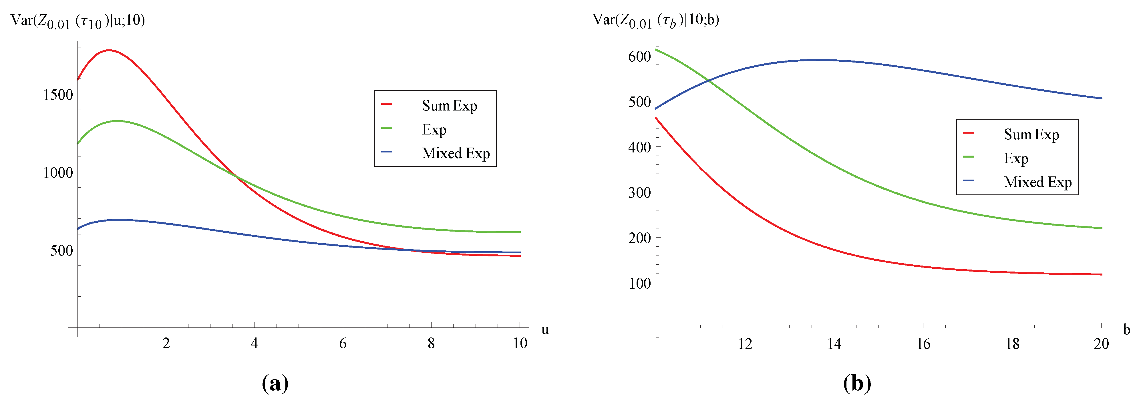
survives longer in expectation, it is natural that on average, more claims occur before ruin. Next, we look at the variance of Z 0 . 01 ( τ b ) , which is shown in Figure 2. Unfortunately, 
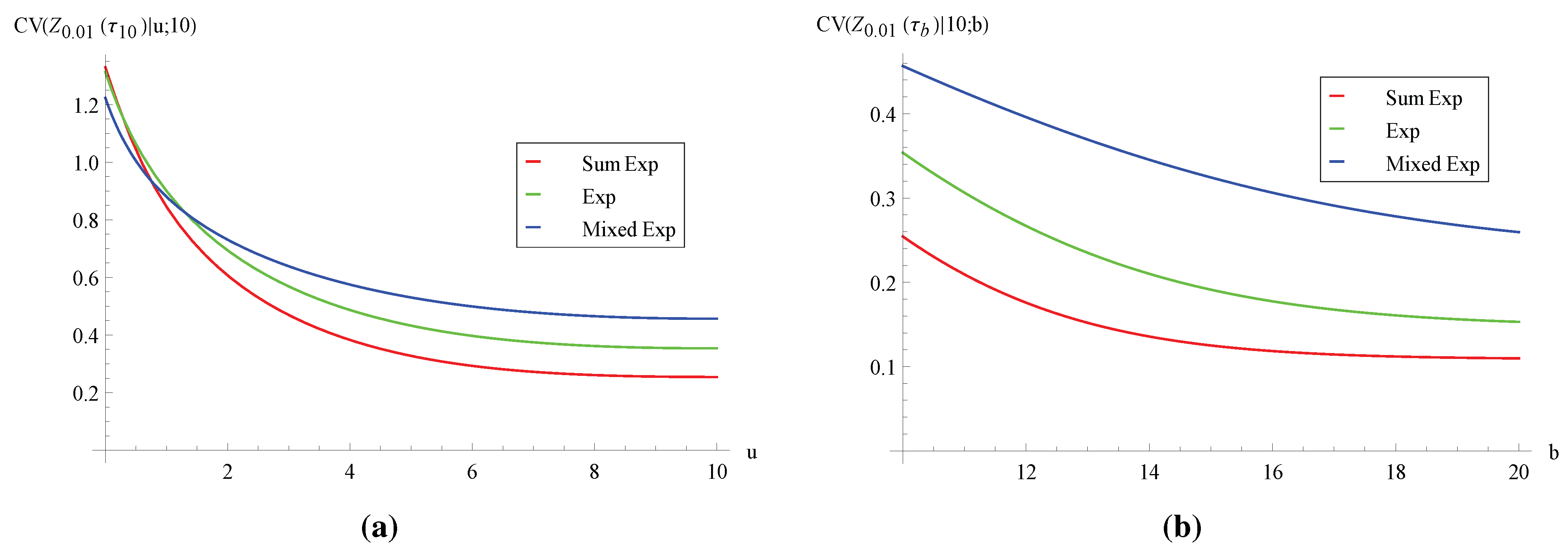
Figure 2 does not appear to show much of a pattern that allows for interpretation. However, if we turn to the coefficient of variation in Figure 3, it can be seen that CV ( Z 0 . 01 ( τ 10 ) | u ; 10 ) and CV ( Z 0 . 01 ( τ b ) | 10 ; b ) are decreasing in u and b, respectively. Furthermore, Figure 3 suggests that CV ( Z 0 . 01 ( τ b ) | u ; b ) increases with the variance of the claim distribution (with the exception of small values of u in Figure 3a). In other words, once we have used a standardized measure of dispersion, which is unitless, the variability of the aggregate discounted claims until ruin Z 0 . 01 ( τ b ) is in accordance with that of the individual claim.
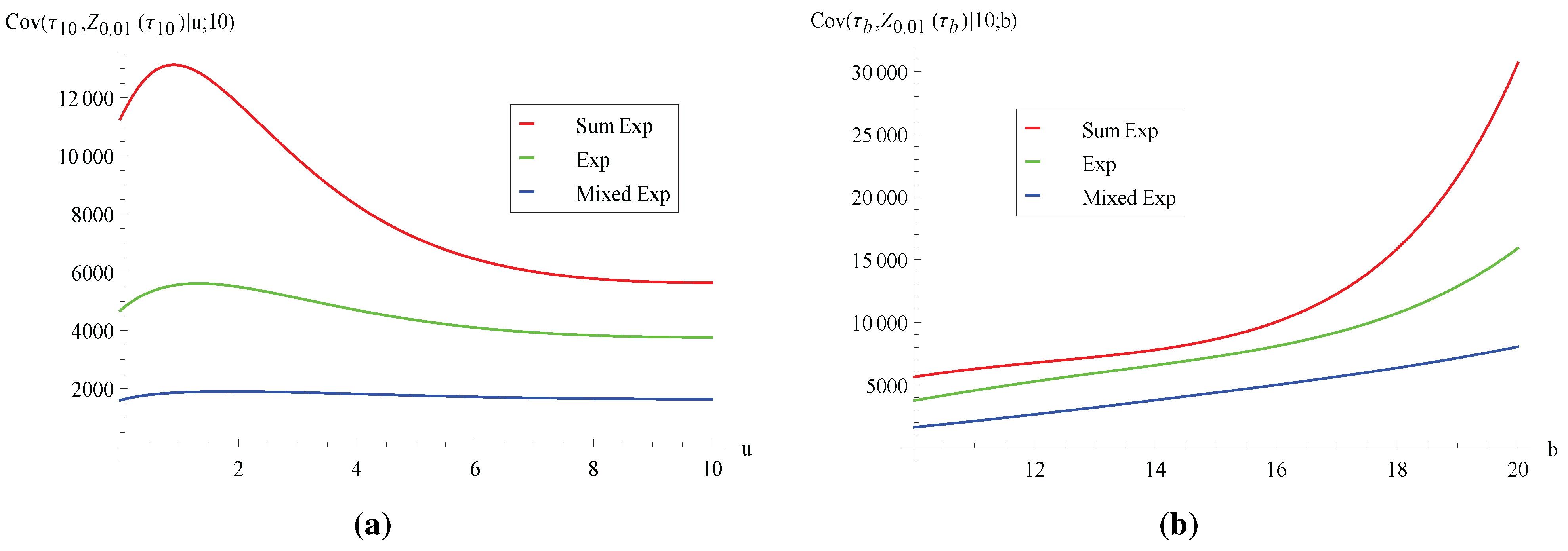
After analyzing the first two moments of Z 0 . 01 ( τ b ) , we now look at various covariance measures. Concerning the relationship between the ruin time τ b and the aggregate discounted claims Z 0 . 01 ( τ b ) for fixed ( u , b ) , consider sample paths of the surplus process { U b ( t ) } t 0 for which τ b is large (e.g., larger than the mean E [ τ b | u ; b ] ). Intuitively, there are two opposing effects on Z 0 . 01 ( τ b ) . A longer ruin time means more time for claims to occur, and this tends to increase Z 0 . 01 ( τ b ) . On the other hand, it also implies that no claims larger than b occur early, and this may make Z 0 . 01 ( τ b ) smaller in the presence of discounting. Figure 4 shows that the covariance of τ b and Z 0 . 01 ( τ b ) is positive, suggesting that the former effect dominates under our parameter setting (interested readers are referred to [16] (Section 5) for an example where the latter effect dominates and leads to negative covariance in the context of a dependent Sparre–Andersen model without dividends). In addition, we see from Figure 4 that Cov ( τ b , Z 0 . 01 ( τ b ) | u ; b ) decreases as the variance of individual claims increases. This can be attributed to the fact that, according to our discussions following Figure 1, both τ b and Z 0 . 01 ( τ b ) 
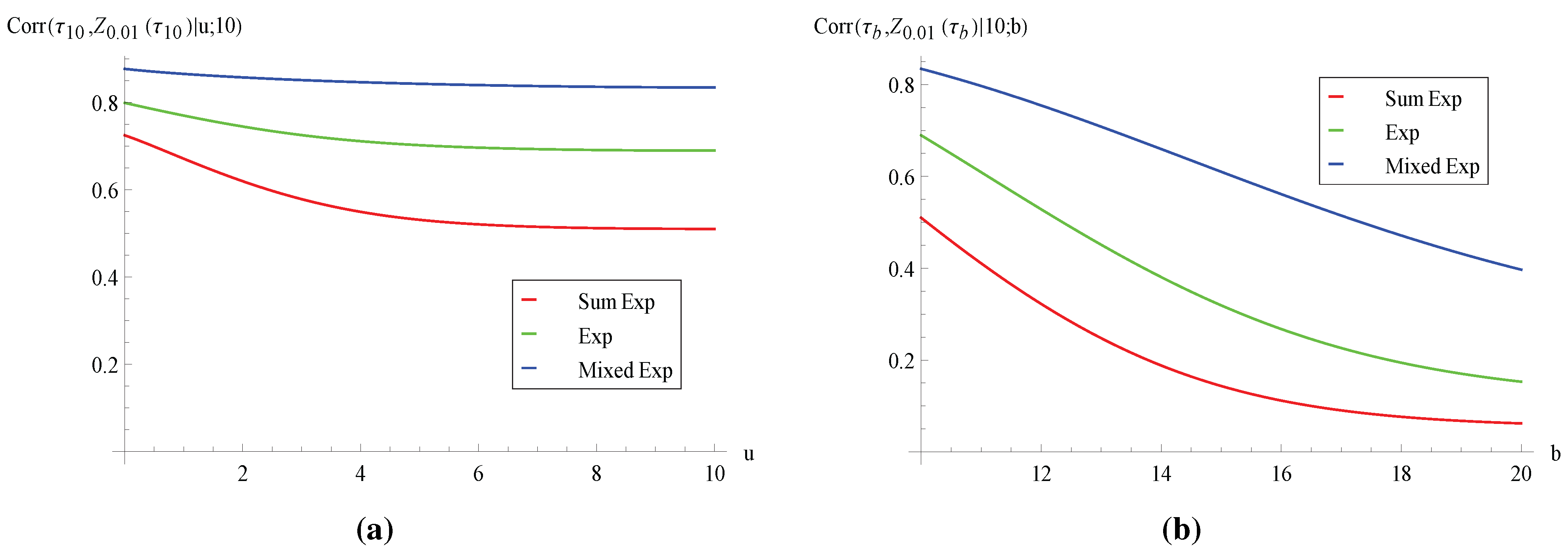
are of a larger magnitude when the claim distribution has smaller variance. In order to remove the effect of different magnitudes, we plot the correlation Corr ( τ b , Z 0 . 01 ( τ b ) | u ; b ) in Figure 5. It is instructive to note that the ordering with respect to the claim’s variance is now reversed, i.e., Corr ( τ b , Z 0 . 01 ( τ b ) | u ; b ) increases with the variance of the claim. Moreover, Corr ( τ b , Z 0 . 01 ( τ b ) | u ; b ) is decreasing in both u and b. Note also that the correlation can sometimes reach 0.8, suggesting that τ b and Z 0 . 01 ( τ b ) can be strongly dependent. Now, we turn to the co-movement of the ruin time τ b and the total discounted dividends D 0 . 01 ( τ b ) . The covariance Cov ( τ b , D 0 . 01 ( τ b ) | u ; b ) in Figure 6 is always positive. Clearly, a larger ruin time means that the insurance business survives longer, and hence, the process { U b ( t ) } t 0 stays at the barrier more often for dividends to be paid. It is also observed from Figure 6 and Figure 7 that both the covariance and the correlation exhibit the same behavior as in Figure 4 and Figure 5 in terms of the shape and ordering of the curves.
Finally, we consider the covariance and the correlation of the aggregate discounted claims Z 0 . 01 ( τ b ) and the total discounted dividends D 0 . 01 ( τ b ) in Figure 8 and Figure 9. Although the covariance Cov ( Z 0 . 01 ( τ 10 ) , D 0 . 01 ( τ 10 ) | u ; 10 ) in Figure 8a is always positive, Cov ( Z 0 . 01 ( τ b ) , D 0 . 01 ( τ b ) | 10 ; b ) in Figure 8b takes negative values as b gets larger when the claim distribution is exponential or a sum of two exponentials. The fact that the covariance is possibly negative may be explained as follows. For fixed ( u , b ) , we already know from previous discussions that both Z 0 . 01 ( τ b ) and D 0 . 01 ( τ b ) tend to be larger when τ b is large. Meanwhile, it should be noted that both claims and dividends are paid from the insurer’s surplus (which consists of the initial surplus plus the premium collected to date). In this regard, one can argue that Z 0 . 01 ( τ b ) and D 0 . 01 ( τ b ) may also move in opposite directions. If the covariance is negative, then it means that the latter effect dominates. While the curves in Figure 8a and Figure 9a as a function of u are not ranked according to the variance of the claim distribution, those in Figure 8b and Figure 9b as a function of b suggest that both covariance and correlation increase with the claim’s variance (except for a very, very small portion in Figure 8b, where the green line is slightly above the blue line when b is close to 10).

Acknowledgments

The authors are grateful to two anonymous referees for their comments on the paper and for pointing out some useful references in the literature. Eric Cheung gratefully acknowledges the support from the Research Grants Council of the Hong Kong Special Administrative Region (Project Number: HKU 701212P). This work is also partially supported by the CAE2013 research grant from the Society of Actuaries. Any opinions, findings and conclusions or recommendations expressed in this material are those of the authors and do not necessarily reflect the views of the SOA.

Author Contributions

All authors contributed equally in all aspects of this work.

Conflicts of Interest

The authors declare no conflict of interest.

References

  1. N.L. Bowers, H.U. Gerber, J.C. Hickman, D.A. Jones, and C.J. Nesbitt. Actuarial Mathematics, 2nd ed. Itasca, IL, USA: The Society of Actuaries, 1997. [Google Scholar]
  2. S.A. Klugman, H.H. Panjer, and G.E. Willmot. Loss Models: From Data to Decisions, 4th ed. Hoboken, NJ, USA: John Wiley & Sons, 2012. [Google Scholar]
  3. H.U. Gerber. “The discounted central limit theorem and its Berry-Esséen analogue.” Ann. Math. Stat. 42 (1971): 389–392. [Google Scholar] [CrossRef]
  4. H.U. Gerber. “Der Einfluss von Zins auf die Ruinwahrscheinlichkeit.” Bull. Swiss Asso. Actuar. 71 (1971): 63–70. [Google Scholar]
  5. G.C. Taylor. “Probability of ruin under inflationary conditions or under experience rating.” ASTIN Bull. 10 (1979): 149–162. [Google Scholar]
  6. G.E. Willmot. “The total claims distribution under inflationary conditions.” Scand. Actuar. J. 1 (1989): 1–12. [Google Scholar] [CrossRef]
  7. G. Léveillé, and J. Garrido. “Recursive moments of compound renewal sums with discounted claims.” Scand. Actuar. J. 2 (2001): 98–110. [Google Scholar] [CrossRef]
  8. J. Li, D.C.M. Dickson, and S. Li. “A note on the distribution of the aggregate claim amount at ruin, 2014.” Available online: http://www.webcitation.org/6c7ZH8ydP (accessed on 9 October 2015).
  9. L. Rabehasaina, and C.C.L. Tsai. “Ruin time and aggregate claim amount up to ruin time for the perturbed risk process.” Scand. Actuar. J. 3 (2013): 186–212. [Google Scholar] [CrossRef]
  10. J. Cai, R. Feng, and G.E. Willmot. “On the expectation of total discounted operating costs up to default and its applications.” Adv. Appl. Probab. 41 (2009): 495–522. [Google Scholar] [CrossRef]
  11. R. Feng. “On the total operating costs up to default in a renewal risk model.” Insur. Math. Econ. 45 (2009): 305–314. [Google Scholar] [CrossRef]
  12. R. Feng. “A matrix operator approach to the analysis of ruin-related quantities in the phase-type renewal risk model.” Bull. Swiss Asso. Actuar. 2009 (2009): 71–87. [Google Scholar]
  13. E.C.K. Cheung, and R. Feng. “A unified analysis of claim costs up to ruin in a Markovian arrival risk process.” Insur. Math. Econ. 53 (2013): 98–109. [Google Scholar] [CrossRef] [Green Version]
  14. S. Asmussen. Applied Probability and Queues, 2nd ed. New York, NY, USA: Springer, 2003. [Google Scholar]
  15. E.C.K. Cheung. “Moments of discounted aggregate claim costs until ruin in a Sparre Andersen risk model with general inter-claim times.” Insur. Math. Econ. 53 (2013): 343–354. [Google Scholar] [CrossRef]
  16. E.C.K. Cheung, and J.-K. Woo. “On the discounted aggregate claim costs until ruin in dependent Sparre Andersen risk processes.” Scand. Actuar. J., 2014, in press. [Google Scholar] [CrossRef] [Green Version]
  17. H. Albrecher, and J.L. Teugels. “Exponential behavior in the presence of dependence in risk theory.” J. Appl. Probab. 43 (2006): 257–273. [Google Scholar] [CrossRef]
  18. A.E. Kyprianou, and Z. Palmowski. “Distributional study of De Finetti’s dividend problem for a general Lévy insurance risk process.” J. Appl. Probab. 44 (2007): 428–443. [Google Scholar] [CrossRef]
  19. H.U. Gerber, and E.S.W. Shiu. “On the time value of ruin.” N. Am. Actuar. J. 2 (1998): 48–72. [Google Scholar] [CrossRef]
  20. B. De Finetti. “Su un’impostazione alternativa della teoria collettiva del rischio.” Trans. XVth Int. Congr. Actuar. 2 (1957): 433–443. [Google Scholar]
  21. H.U. Gerber. An Introduction to Mathematical Risk Theory. Edited by R.D. Irwin. Homewood, IL, USA: Huebner Foundation, 1979. [Google Scholar]
  22. R.L. Loeffen. “On optimality of the barrier strategy in de Finetti’s dividend problem for spectrally negative Lévy processes.” Ann. Appl. Probab. 18 (2008): 1669–1680. [Google Scholar] [CrossRef]
  23. X.S. Lin, G.E. Willmot, and S. Drekic. “The compound Poisson risk model with a constant dividend barrier: analysis of the Gerber–Shiu discounted penalty function.” Insur. Math. Econ. 33 (2003): 551–566. [Google Scholar]
  24. D.C.M. Dickson, and H.R. Waters. “Some optimal dividends problems.” ASTIN Bull. 34 (2004): 49–74. [Google Scholar] [CrossRef]
  25. H.U. Gerber, E.S.W. Shiu, and N. Smith. “Maximizing dividends without bankruptcy.” ASTIN Bull. 36 (2006): 5–23. [Google Scholar] [CrossRef]
  26. J.-F. Renaud, and X. Zhou. “Distribution of the present value of dividend payments in a Lévy risk model.” J. Appl. Probab. 44 (2007): 420–427. [Google Scholar] [CrossRef]
  27. H. Albrecher, and H.U. Gerber. “A note on moments of dividends.” Acta Math. Appl. Sin. 27 (2011): 353–354. [Google Scholar] [CrossRef]
  28. H.U. Gerber, X.S. Lin, and H. Yang. “A note on the dividends-penalty identity and the optimal dividend barrier.” ASTIN Bull. 36 (2006): 489–503. [Google Scholar] [CrossRef]
  29. E.C.K. Cheung, and D. Landriault. “A generalized penalty function with the maximum surplus prior to ruin in a MAP risk model.” Insur. Math. Econ. 46 (2010): 127–134. [Google Scholar] [CrossRef]
  30. A.E. Kyprianou. Gerber–Shiu Risk Theory. Heidelberg, Germany: Springer, 2013. [Google Scholar]
  31. D. Dufresne. “Fitting combinations of exponentials to probability distributions.” Appl. Stoch. Mod. Bus. Ind. 23 (2007): 23–48. [Google Scholar] [CrossRef]
  32. D.C.M. Dickson, and C. Hipp. “On the time to ruin for Erlang(2) risk processes.” Insur. Math. Econ. 29 (2001): 333–344. [Google Scholar] [CrossRef]
  33. S. Li, and J. Garrido. “On ruin for the Erlang(n) risk process.” Insur. Math. Econ. 34 (2004): 391–408. [Google Scholar] [CrossRef]

