Production Flexibility and Hedging

Abstract

We extend the analysis on hedging with price and output uncertainty by endogenizing the output decision. Specifically, we consider the joint determination of output and hedging in the case of flexibility in production. We show that the risk-averse firm always maintains a short position in the futures market when the futures price is actuarially fair. Moreover, in the context of an example, we show that the presence of production flexibility reduces the incentive to hedge for all risk averse agents.

1. Introduction

Analyses of hedging decisions by non-financial firms emerged in the economics literature in the late 1970s (see for instance Holthausen [1] and Feder et al. [2]). In articles published since then, all decisions are made simultaneously and derivatives are used to hedge a price risk (input or output). Under general conditions, including a concave payoff, a separation holds between production decision and hedging decision when there is no basis risk or production uncertainty [3].

An extension of this literature allows firms to consider production decisions after uncertainty is resolved. Many firms face price and output uncertainty in different markets. Few articles have studied this difficult problem without assuming a mean-variance framework. As Moschini and Lapan [4] argue, this limited framework does not take into account all features of production flexibility, particularly the fact that the firm profit function is non-linear in the risky price. Their contribution focuses on the choice of different derivative instruments in the presence of this non-linearity. They show that the use of options is welfare improving and affects input decisions when the profit function is convex in price and the distribution of price is symmetric. We do not consider the types of derivatives in our analysis. However, we use the same assumptions of profit convexity in price and symmetry of the price distribution to obtain our result regarding the hedging component.

In a different framework with an exogenous and random output, Losq [5] provides two important results about the hedging component of the optimal volume of futures contracts. First, the hedging component is short (long) when demand is elastic (inelastic). Second, in the case of stochastic independence between price and output, the hedging component is less than expected output if and only if the utility exhibits prudence. This article extends Losq [5] by endogenizing the output decision in the case of production flexibility. Because production flexibility yields price and output uncertainty, we can compare our results with those of Losq [5].

We show that the endogenization of output with production flexibility alters the results. In the context of price and output uncertainty, our results related to hedging complement those of Losq [5], who examined exogenous production. First, when the futures price is actuarially fair, the hedging component is always positive due to risk aversion, contrary to Losq [5], who found that the optimal hedging component is conditional on demand elasticity. In our paper, when real and hedging decisions are made jointly, demand and production have no influence on the hedging component. Second, because we consider endogenous production we cannot analyze the case of stochastic independence between price and output. Unlike Losq [5], we show that the hedging component of a risk-averse decision maker is always lower than the expected output. Because of the additional difficulty of production flexibility, we show our result assuming a symmetric binary distribution. Moreover, our result shows that prudence is not a determinant of the ordering of the hedging component and expected output when production is flexible. In other words, in our framework, it is the presence of production flexibility, rather than prudence, that reduces the incentive to hedge because production flexibility is a form of natural hedging and becomes a substitute for financial hedging.

The rest of the article is organized as follows. Section 2 presents the model. Section 3 derives and analyzes the main results. A short conclusion summarizes our main results and proposes a possible extension to our contribution.

2. Model

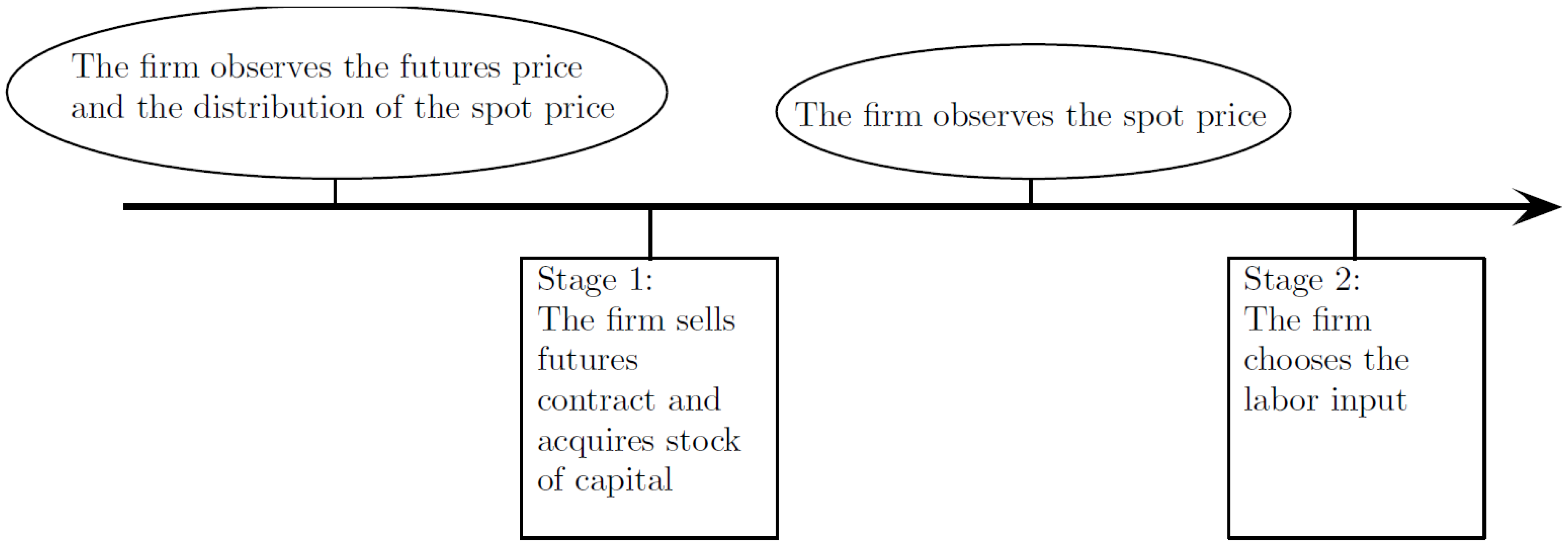
We embed production flexibility in a two-stage maximization problem. At the first stage, the firm sets the volume of futures contracts and acquires the stock of capital while facing uncertainty about the spot price of the output. At the second stage, given the volume of futures contracts and the capital stock, the firm observes the spot price of the output, and then chooses labor. Figure 1 describes the timeline of the model. Specifically, the ellipses above the line provides information about what the firm observes prior to each stage. The rectangles below the line describes the choices of the firm at each stage.

Figure 1. Timeline.

Figure 1. Timeline.

We now provide a detailed description of the model. Consider a perfectly competitive firm acquiring l units of labor and k units of capital, which produces q units of output. The technology to transform input into output is defined by $q=\phi (k,l)$ with ${\phi }_1,{\phi }_2,{\phi }_{12}>0$ and ${\phi }_{11},{\phi }_{22}<0$. Total cost functions for labor and capital are $c_l\left(l\right)$ and $c_k\left(k\right)$, respectively, such that $c_l^{\prime },c_k^{\prime }>0$ and $c_l^{″},c_k^{″}\ge 0$.

The firm sells x units of output on the futures market at price F, and sells the remaining $\phi (k,l)-x$ units on the spot market at price S. Given the firm’s decisions $\{k,l,x\}$ and the prices $\{S,F\}$, the profit function is

$$\pi (k,l,x,S,F)=S\phi (k,l)-c_l\left(l\right)-c_k\left(k\right)+(F-S)x$$

(1)

where $S\phi (k,l)$ is the revenue from selling $\phi (k,l)$ units of output at spot price S, $c_l\left(l\right)+c_k\left(k\right)$ is the total cost of production, and $(F-S)x$ is the financial profit due to selling x units of output at futures price F instead of spot price S. Equation (1) can thus be written alternatively as $\pi (k,l,x,S,F)=S(\phi (k,l)-x)+Fx-c_l\left(l\right)-c_k\left(k\right)$ where $S\left(\phi \right(k,l)-x)$ is the revenue from the spot market and $Fx$ is the revenue from the futures market.

A risk-averse manager makes decisions so as to maximize the expected utility of profit.1 His objective function is $u\left(\pi \right(k,l,x,S,F\left)\right)$ such that $u^{\prime }>0$, $u^{″}<0$. The uncertainty comes from the spot price. Let $\tilde{S}$ be the random spot price and $\mu =\mathbb{E}[\tilde{S}]$ be the expected spot price where $\mathbb{E}[·]$ is the expectation operator and a tilde distinguishes a random variable from a realization.

Capital is set prior to observing the spot price whereas labor is chosen after the spot price is known. In other words, the choice of capital depends on expectations about the spot price whereas the choice of labor depends on the realized spot price. In our model, production is flexible because the firm is able to alter production (through the choice of labor) after the spot price is realized. In many industries, the firms are able to adjust production upon acquiring new information about the spot price. While capital inputs require long-term planning, labor inputs can be adjusted more easily (e.g., temporary layoffs) so as to modify the final level of production. Although the degree of flexibility varies across industries, capital-intensive industries (compared to labor-intensive industries) are in general less able to adjust production. For instance, the gold-mining industry requires long-term planning in production, which significantly reduces capital flexibility.

The maximization problem can be divided into two stages.2 In the first stage, the firm sets the volume of futures contracts and acquires the stock of capital while facing uncertainty about the spot price. In the second stage, the firm observes the spot price and chooses labor, which determines output.

We now define the two-stage maximization problem. Since Stage 1 precedes Stage 2, the solution for labor (in Stage 2) depends on the solutions for capital and futures contracts as well as the realization of the spot price. Note that production flexibility yields uncertainty in production through the optimal choice of labor. Hence, the maximization problem in Stage 1 requires taking an expectation over the random spot price.

Definition 1. 

The pair $\{l^{*}(k^{*},x^{*},S),k^{*},x^{*}\}$ satisfies,

• In stage 2, given $\{k^{*},x^{*}\}$ and S,

  $$l^{*}(k^{*},x^{*},S)=arg\underset{l}{max}u(S\phi (k^{*},l)-c_l\left(l\right)-c_k\left(k^{*}\right)+(F-S)x^{*})$$

  (2)
• In stage 1, given $l^{*}(k,x,S)$,

  $$\{k^{*},x^{*}\}=arg\underset{k,x}{max}\mathbb{E}[u({\Pi }^{*}(k,x,\tilde{S}))]$$

  (3)

  where ${\Pi }^{*}(k,x,\tilde{S})=\tilde{S}\phi (k,l^{*}(k,x,\tilde{S}))-c_l(l^{*}(k,x,\tilde{S}))-c_k\left(k\right)+(F-\tilde{S})x$

.

Having described the set up, we derive the optimal behavior of the firm. We first provide the solution to the second stage. It turns out that the solution for labor is independent of futures contracts, but depends on both the capital and the spot price. To simplify notation, we write $l^{*}(k^{*},S)\equiv l^{*}(k^{*},x^{*},S)$.

Proposition 1. 

In Stage 2, $l^{*}(k^{*},S)$ satisfies

$$S{\phi }_2(k,l^{*}(k^{*},S))-c_l^{\prime }\left(l^{*}(k^{*},S)\right)=0$$

(4)

Proof. 

Since $u^{\prime }>0$, the maximization problem defined in Equation (2) is equivalent to

$$\underset{l}{max}\{S\phi (k^{*},l)-c_l\left(l\right)-c_k\left(k^{*}\right)+(F-S)x^{*}\}$$

(5)

The first-order condition yields Equation (4), and, thus, optimal labor depends on $k^{*}$ and S, but not $x^{*}$. The second-order condition is satisfied, i.e., $u^{″}<0$ and $S{\phi }_{22}(k^{*},l)-c_l^{″}\left(l\right)<0$ for all l and thus, Equation (4) yields a unique global maximizer.  ☐

Having solved for Stage 2, we use the solution for labor to solve for the maximization problem in Stage 1. In order to compare our results with Losq [5], we follow Losq [5] by focusing on an interior solution and by assuming that the Hessian of the maximization problem is negative definite. Note that risk aversion and properties of the production functions alone are not enough to ensure an interior solution in the case of production flexibility. To see this, let $V(k,x)\equiv \mathbb{E}[u({\Pi }^{*}(k,x,\tilde{S}))]$. It is true that $V{}_{11}(k,x)<0$ and $V{}_{22}(k,x)<0$. 3 However,

$$\begin{array}{cc}& V_{11}(k,x)V_{22}(k,x)-{\left[V_{21}(k,x)\right]}^2\hfill \\ \hfill =& \mathbb{E}[{\Pi }_{11}^{*}(k,x,\tilde{S})u^{\prime }({\Pi }^{*}(k,x,\tilde{S}))+{({\Pi }_1^{*}(k,x,\tilde{S}))}^2{u}^{″}({\Pi }^{*}(k,x,\tilde{S}))]\hfill \\ & ·\mathbb{E}[{({\Pi }_2^{*}(k,x,\tilde{S}))}^2{u}^{″}({\Pi }^{*}(k,x,\tilde{S}))]\hfill \\ & -{(\mathbb{E}[{\Pi }_2^{*}(k,x,\tilde{S}){\Pi }_1^{*}(k,x,\tilde{S})u^{\prime }({\Pi }^{*}(k,x,\tilde{S}))])}^2\hfill \end{array}$$

(8)

is not easily signed.

Proposition 2. 

Suppose that the Hessian of $\mathbb{E}[u({\Pi }^{*}(k,x,\tilde{S}))]$ is negative definite. In Stage 1, $\{k^{*},x^{*}\}$ satisfy

$$\begin{array}{cc}& \mathbb{E}[(\tilde{S}{\phi }_1(k^{*},l^{*}(k^{*},\tilde{S}))-c_k^{\prime }\left(k^{*}\right))u^{\prime }({\Pi }^{*}(k^{*},x^{*},\tilde{S}))]=0\hfill \end{array}$$

(9)

$$\begin{array}{cc}& \mathbb{E}[(F-\tilde{S})u^{\prime }({\Pi }^{*}(k^{*},x^{*},\tilde{S}))]=0\hfill \end{array}$$

(10)

Proof. 

The first-order conditions corresponding to Equation (3) yield Equations (9) and (10). Since the Hessian is assumed to be negative definite, the first-order conditions yield a maximizer.  ☐

3. Analysis

In this section, we compare our results with Losq [5].

Short vs. Long Hedging. We first consider the issue of short hedging versus long hedging. The firm maintains a short position (long position) when the hedging component of the optimal volume of futures contracts is strictly positive (strictly negative). With exogenous and random output, Losq [5] shows that the hedging component is short (long) when demand is elastic (inelastic). We show that the endogenization of output in the presence of production flexibility alters the result.

As in Losq [5], we can decompose $x^{*}$ into two components. Specifically, Proposition 3 provides the hedging and speculative components of the optimal volume of futures contracts. We then ascertain the sign of the hedging component in Proposition 4.

Proposition 3. 

The optimal volume of futures contracts can be decomposed as $x^{*}=x_s^{*}+x_h^{*}$ where

$$x_s^{*}=-\frac{\mathbb{E}[u^{\prime }({\Pi }^{*}(k^{*},x^{*},\tilde{S}))](F-\mu )}{\mathbb{E}[{(\tilde{S}-\mu )}^2{u}^{″}({\Pi }^{*}(k^{*},x^{*},F(\tilde{S})))]}$$

(11)

is the speculative component and

$$x_h^{*}=\frac{\mathbb{E}[{(\tilde{S}-\mu )}^2{u}^{″}({\Pi }^{*}(k^{*},x^{*},F(\tilde{S})))\phi (k^{*},l^{*}(k^{*},F(\tilde{S})))]}{\mathbb{E}[{(\tilde{S}-\mu )}^2{u}^{″}({\Pi }^{*}(k^{*},x^{*},F(\tilde{S})))]}$$

(12)

is the hedging component. Here, $F(\tilde{S})\in (min\{\tilde{S},\mu \},max\{\tilde{S},\mu \})$.

Proof. 

Equation (10) is rewritten as

$$\mathbb{E}[u^{\prime }({\Pi }^{*}(k^{*},x^{*},\tilde{S}))](F-\mu )-\mathbb{E}[u^{\prime }({\Pi }^{*}(k^{*},x^{*},\tilde{S}))(\tilde{S}-\mu )]=0$$

(13)

with ${\Pi }^{*}(k^{*},x^{*},\tilde{S})=\tilde{S}\phi (k^{*},l^{*}(k^{*},\tilde{S}))-c_l(l^{*}(k^{*},\tilde{S}))-c_k(k^{*})+(F-\tilde{S})x^{*}$. Letting $g(\tilde{S})=u^{\prime }({\Pi }^{*}(k^{*},x^{*},\tilde{S}))$ and using the mean-value theorem, we can find a function $F(\tilde{S})$ between $\tilde{S}$ and μ so that

$$g(\tilde{S})=g\left(\mu \right)+(\tilde{S}-\mu )g^{\prime }(F(\tilde{S}))$$

(14)

Plugging Equation (14) into Equation (13) yields $\mathbb{E}[u^{\prime }({\Pi }^{*}(k^{*},x^{*},\tilde{S}))](F-\mu )-\mathbb{E}[(g(\mu )+(\tilde{S}-\mu )g^{\prime }(F(\tilde{S})))(\tilde{S}-\mu )]=0$, which simplifies to (using $\mu =\mathbb{E}[\tilde{S}]$)

$$\mathbb{E}[u^{\prime }({\Pi }^{*}(k^{*},x^{*},\tilde{S}))](F-\mu )-\mathbb{E}[{(\tilde{S}-\mu )}^2{g}^{\prime }(F(\tilde{S}))]=0$$

(15)

The derivation is similar to the one found in Losq [5] with a crucial difference. The difference lies in the expression $g^{\prime }(F(\tilde{S}))$ in Equation (15). Specifically, given that $g(\tilde{S})=u^{\prime }({\Pi }^{*}(k^{*},x^{*},\tilde{S}))$,

$$\begin{array}{cc}\hfill g^{\prime }(F(\tilde{S}))=& u^{″}({\Pi }^{*}(k^{*},x^{*},F(\tilde{S})))\hfill \\ & (\phi (k^{*},l^{*}(k^{*},F(\tilde{S})))+F(\tilde{S}){\phi }_2(k^{*},l^{*}(k^{*},F(\tilde{S})))-c_l^{\prime }(l^{*}(k^{*},F(\tilde{S})))-x^{*})\hfill \end{array}$$

(16)

The term $\phi (k^{*},l^{*}(k^{*},F(\tilde{S})))+F(\tilde{S}){\phi }_2(k^{*},l^{*}(k^{*},F(\tilde{S})))$ in Equation (16) is reminiscent of the elasticity-of-demand term in Losq [5]. However, in our case, the endogenization of production through labor removes the link between production and hedging. That is, using Equation (4), Equation (16) is rewritten as

$$g^{\prime }(F(\tilde{S}))=u^{″}({\Pi }^{*}(k^{*},x^{*},F(\tilde{S})))(\phi (k^{*},l^{*}(k^{*},F(\tilde{S})))-x^{*})$$

(17)

Plugging Equation (17) into Equation (15) and solving for optimal volume of futures contracts yields $x^{*}=x_s^{*}+x_h^{*}$ where $x_s^{*}$ and $x_h^{*}$ are defined by Equation (11) and Equation (12), respectively.  ☐

As usual, the speculative term depends on the bias of the spot price. (i.e., $x_s^{*}>0\iff F>\mu$). Proposition 4 states that, in contrast to Losq [5], the hedging component is always positive due to risk aversion (i.e., $u^{″}<0$). In other words, when real and financial decisions are jointly made, demand and production have no influence on the sign of the hedging component. Note that in our model with production flexibility, risk aversion is a necessary and sufficient condition for the hedging component to be positive.

Proposition 4. 

Under production flexibility, the risk-averse firm always maintains a short position in the futures market, i.e., $x_h^{*}>0$.

Proof. 

From Equation (12), risk aversion (i.e., $u^{″}<0$) implies $x_h^{*}>0$.  ☐

Optimal Expected Output and Optimal Hedging. In a model with price uncertainty and no production flexibility, the full-hedging result states that output is equal to the hedging component and there is no speculative component [1,2,3,8].

In the case of price and output uncertainty, the full-hedging result compares the hedging component with expected output. With exogenous output, when price and output uncertainty are stochastically independent, Losq [5] establishes that the hedging component is less than expected output if and only if the manager is prudent (i.e., $u^{‴}>0$). In the context of an example, we show that, under risk aversion, the hedging component is always less than expected output in the case of endogenous output with production flexibility. This means that prudence is not necessary to get the same result in our more flexible environment.

Focusing on the hedging component, Equation (12) is rewritten as

$$x_h^{*}=\overline{Q}+\frac{\mathbb{E}[{(\tilde{S}-\mu )}^2{u}^{″}({\Pi }^{*}(k^{*},x^{*},F(\tilde{S})))(\phi (k^{*},l^{*}(k^{*},F(\tilde{S})))-\overline{Q})]}{\mathbb{E}[{(\tilde{S}-\mu )}^2{u}^{″}({\Pi }^{*}(k^{*},x^{*},F(\tilde{S})))]}$$

(18)

where $\overline{Q}=\mathbb{E}[\phi (k^{*},l^{*}(k^{*},\tilde{S}))]$ is expected output. Using the covariance operator, Equation (18) is rewritten as

$$\begin{array}{cc}\hfill x_h^{*}=& \overline{Q}+\frac{\mathbb{E}[{(\tilde{S}-\mu )}^2{u}^{″}({\Pi }^{*}(k^{*},x^{*},F(\tilde{S})))]\mathbb{E}[(\phi (k^{*},l^{*}(k^{*},F(\tilde{S})))-\overline{Q})]}{\mathbb{E}]{(\tilde{S}-\mu )}^2{u}^{″}({\Pi }^{*}(k^{*},x^{*},F(\tilde{S})))]}\hfill \\ & +\frac{\mathbf{COV}[{(\tilde{S}-\mu )}^2{u}^{″}({\Pi }^{*}(k^{*},x^{*},F(\tilde{S}))),\phi (k^{*},l^{*}(k^{*},F(\tilde{S})))]}{\mathbb{E}[{(\tilde{S}-\mu )}^2{u}^{″}({\Pi }^{*}(k^{*},x^{*},F(\tilde{S})))]}\hfill \end{array}$$

(19)

where recall that $F(\tilde{S})\in (min\{\tilde{S},\mu \},max\{\tilde{S},\mu \})$ and ${\Pi }^{*}(k^{*},x^{*},F(\tilde{S}))=F(\tilde{S})\phi (k^{*},l^{*}(k^{*},F(\tilde{S})))-c_l(l^{*}(k^{*},F(\tilde{S})))-c_k(k^{*})+(F-F(\tilde{S}))x^{*}$. From Equation (19), the firm does not necessarily hedge all expected production. In our case, the presence of production flexibility implies that unlike Losq [5] we cannot remove the second term and simplify the third term in Equation (19). Indeed, through the choice of labor, $\tilde{S}$ and $\phi (k^{*},l^{*}(k^{*},\tilde{S}))$ are dependent on each other since the randomness in output is due to the randomness in the spot price through the choice of labor. In other words, $\tilde{S}$ and $\phi (k^{*},l^{*}(k^{*},\tilde{S}))$ are in general unconditionally dependent, i.e., when we consider ex ante production before the spot price is realized.

In order to investigate whether prudence matters in the case of endogenous production, the problem must be simplified. That is, we consider a specific example. Unlike Losq [5], we cannot take the route of making price and output independent since production flexibility prohibits this case. Rather, we consider the case of a symmetric binary distribution for the spot price while retaining stochastic dependence between price and output. Proposition 5 states that the hedging component of a risk-averse agent is less than expected output. The reason is that hedging and flexibility in production are substitutes. That is, flexibility in production reduces the benefit of hedging.4 Moreover, our result shows that prudence is not a determinant of the ordering of the hedging component and expected output when production is flexible.

Proposition 5. 

Suppose that for $\epsilon \in (0,F)$, $Pr[\tilde{S}=F-\epsilon ]=Pr[\tilde{S}=F+\epsilon ]=1/2$. Then, the hedging component of a risk-averse agent is less than expected output, i.e., such that $0<x_h^{*}<\overline{Q}$.

Proof. 

First, given the binary distribution and the fact that $u^{″}<0$, Equation (10) is rewritten as

$$\begin{array}{c}{u}^{\prime }((F-\epsilon )\phi (k,l^{*}(k,F-\epsilon ))-c_l\left(l^{*}(k,F-\epsilon )\right)-c_k\left(k\right)+\epsilon x)\hfill \\ =u^{\prime }((F+\epsilon )\phi (k,l^{*}(k,F+\epsilon ))-c_l\left(l^{*}(k,F+\epsilon )\right)-c_k\left(k\right)-\epsilon x)\hfill \end{array}$$

(20)

where $u^{\prime }>0$. Since $u^{″}<0$ due to risk aversion, Equation (20) yields

$$\begin{array}{cc}\hfill x_h^{*}=& \frac{(F+\epsilon )\phi (k,l^{*}(k,F+\epsilon ))-c_l\left(l^{*}(k,F+\epsilon )\right)}{2\epsilon }\hfill \\ & -\frac{(F-\epsilon )\phi (k,l^{*}(k,F-\epsilon ))-c_l\left(l^{*}(k,F-\epsilon )\right)}{2\epsilon }\hfill \end{array}$$

(21)

From Equation (21) and applying Equation (4), we obtain

$$\begin{array}{cc}\hfill \frac{\partial x_h^{*}}{\partial \epsilon }=& \frac{\phi (k,l^{*}(k,F+\epsilon ))+\phi (k,l^{*}(k,F-\epsilon ))}{2\epsilon }\hfill \\ & +\frac{(F-\epsilon )\phi (k,l^{*}(k,F-\epsilon ))-c_l\left(l^{*}(k,F-\epsilon )\right)}{2{\epsilon }^2}\hfill \\ & -\frac{(F+\epsilon )\phi (k,l^{*}(k,F+\epsilon ))-c_l\left(l^{*}(k,F+\epsilon )\right)}{2{\epsilon }^2}\hfill \end{array}$$

(22)

Let

$$\mathbb{E}\phi (k,l^{*}(k,\tilde{S}))=\frac{\phi (k,l^{*}(k,F+\epsilon ))+\phi (k,l^{*}(k,F-\epsilon ))}{2}$$

(23)

be the expected optimal level of output. Using Equations (21) and (23), Equation (22) is rewritten as

$$\frac{\partial x_h^{*}}{\partial \epsilon }=\frac{\mathbb{E}\phi (k,l^{*}(k,\tilde{S}))-x_h^{*}}{\epsilon }$$

(24)

Second, we find the sign of $\frac{\partial x_h^{*}}{\partial \epsilon }$. Since $u^{″}<0$, Equation (20) is rewritten as

$$\frac{{\Pi }^{*}(k,x,F-\epsilon )}{2}-\frac{{\Pi }^{*}(k,x,F+\epsilon )}{2}=0$$

(25)

where for $S>0$,

$${\Pi }^{*}(k,x,S)=S\phi (k,l^{*}(k,S))-c_l\left(l^{*}(k,S)\right)-c_k\left(k\right)+(F-S)x$$

(26)

Applying Equation (4), $\frac{\partial {\Pi }^{*}(k,x,S)}{\partial S}=\phi (k,l^{*}(k,S))-x$ so that

$$\frac{{\partial }^2{\Pi }^{*}(k,x,S)}{\partial S^2}={\phi }_2(k,l^{*}(k,S))\frac{\partial l^{*}(k,S)}{\partial S}>0$$

(27)

since, from Equation (4), $\frac{\partial l^{*}(k,S)}{\partial S}=\frac{-{\phi }_2(k,l^{*}(k,S))}{S{\phi }_{22}(k,l^{*}(k,S))-c_l^{″}\left(l^{*}(k,S)\right)}>0$. Then, by Theorem 1 of Diamond and Stiglitz [10], convexity of ${\Pi }^{*}(k,x,S)$ in S implies that $\frac{\partial x_h^{*}}{\partial \epsilon }>0$. Hence, from Equation (24), $\mathbb{E}\phi (k,l^{*}(k,\tilde{S}))-x_h^{*}>0$ for all k and thus for $k^{*}$. ☐

4. Conclusions

In this paper, we added production flexibility and consequently dependence between price and output to analyze the nature of the hedging component of a firm with a concave payoff facing output price uncertainty. We show that the hedging component is always positive when the futures price is actuarially fair and is independent of demand elasticity. Second, we confirm that the hedging component is always lower than the expected output, a result that is empirically observed in industries that have production flexibility. Hedging and production flexibility are thus imperfect substitutes because firms with a concave payoff always hedge when hedging is actuarially fair.

A potential extension of our research is to analyze the nature of the optimal hedging instruments along with production flexibility. As mentioned, Moschini and Lapan [4] did not consider production flexibility. Recent empirical evidence in the oil and gas industry shows that nonlinear hedging strategies are motivated by sensitivities of firms investment expenditures and revenues to oil price fluctuations, geographical diversification, and quantityprice correlation [11]. Production uncertainty is also shown to play a significant role in hedging strategy choice. However, the results are also a function of the oil and gas market conditions. Extending the analysis of this article to this empirical environment with production flexibility would represent a true challenge.

References

- D.M. Holthausen. “Hedging and the Competitive Firm under Price Uncertainty.” Am. Econ. Rev. 69 (1979): 989–995. [Google Scholar]
- G. Feder, R.E. Just, and A. Schmitz. “Futures Markets and the Theory of the Firm under Price Uncertainty.” Q. J. Econ. 94 (1980): 317–328. [Google Scholar] [CrossRef]
- J.P. Danthine. “Information, Futures Prices, and Stabilizing Speculation.” J. Econ. Theory 17 (1973): 79–98. [Google Scholar] [CrossRef]
- G. Moschini, and H. Lapan. “Hedging Price Risk with Options and Futures for the Competitive Firm with Production Flexibility.” Int. Econ. Rev. 33 (1992): 607–618. [Google Scholar] [CrossRef]
- E. Losq. “Hedging with Price and Output Uncertainty.” Econ. Lett. 10 (1982): 65–70. [Google Scholar] [CrossRef]
- G. Dionne, and M. Santugini. “Entry, Imperfect Competition, and Futures Market for the Input.” Int. J. Ind. Organ. 35 (2014): 70–83. [Google Scholar] [CrossRef]
- T.O. Léautier, and J.C. Rochet. “On the Strategic Value of Risk Management.” Int. J. Ind. Organ. 37 (2014): 153–169. [Google Scholar] [CrossRef]
- W.J. Ethier. “International Trade and the Forward Exchange Market.” Am. Econ. Rev. 63 (1973): 494–503. [Google Scholar]
- P. Tufano. “Who Manages Risk? An Empirical Examination of Risk Management Practices in the Gold Mining Industry.” J. Financ. 51 (1996): 1097–1137. [Google Scholar] [CrossRef]
- P.A. Diamond, and J.E. Stiglitz. “Increases in Risk and in Risk Aversion.” J. Econ. Theory 8 (1974): 337–360. [Google Scholar] [CrossRef]
- M. Mnasri, G. Dionne, and J.P. Gueyie. “How Do Firms Hedge Risks? Empirical Evidence from U.S. Oil and Gas Producers.” 2013. Available online: http://ssrn.com/abstract=2245711 (accessed on 30 November 2015).
- 1Concavity of the payoff function can also be explained by different market imperfections. See Dionne and Santugini [6].
- 2See Léautier and Rochet [7] for a two-stage game in which each firm commits to a hedging strategy in the first stage and then chooses production or pricing strategies in the second stage.
- 3Indeed,where . From Equation (4), so that . Hence, since and . Second,since .
- 4This can explain the behavior of the gold mining industry [9]. In this industry, the firms hedge their selling price for the next three years by using different contracts including forwards and options. It is well documented they hedge only a fraction of their production (the mean of the industry was about in the 1990s) even when their payoff is concave. This means that they keep the flexibility to adjust their production in function of future price fluctuations. In other words, we observe in this industry a trade-off between price protection and production flexibility which rejects full separation. Such trade-off is also observed in the oil and gas industry.
© 2015 by the authors; licensee MDPI, Basel, Switzerland. This article is an open access article distributed under the terms and conditions of the Creative Commons Attribution license (http://creativecommons.org/licenses/by/4.0/).
Share and Cite
MDPI and ACS Style
Dionne, G.; Santugini, M. Production Flexibility and Hedging. Risks 2015, 3, 543-552. https://doi.org/10.3390/risks3040543
AMA Style
Dionne G, Santugini M. Production Flexibility and Hedging. Risks. 2015; 3(4):543-552. https://doi.org/10.3390/risks3040543
Chicago/Turabian StyleDionne, Georges, and Marc Santugini. 2015. "Production Flexibility and Hedging" Risks 3, no. 4: 543-552. https://doi.org/10.3390/risks3040543