
Modified Munich Chain-Ladder Method

1
Faculty of Business Administration, University of Hamburg, 20146 Hamburg, Germany
2
ETH Zurich, RiskLab, Department of Mathematics, 8092 Zurich, Switzerland
*
Author to whom correspondence should be addressed.
†
Swiss Finance Institute SFI Professor.
Risks 2015, 3(4), 624-646; https://doi.org/10.3390/risks3040624
Submission received: 30 September 2015
/
Accepted: 1 December 2015
/
Published: 21 December 2015
(This article belongs to the Special Issue Applying Stochastic Models in Practice: Empirics and Numerics)
Abstract
:The Munich chain-ladder method for claims reserving was introduced by Quarg and Mack on an axiomatic basis. We analyze these axioms, and we define a modified Munich chain-ladder method which is based on an explicit stochastic model. This stochastic model then allows us to consider claims prediction and prediction uncertainty for the Munich chain-ladder method in a consistent way.
1. Introduction
The Munich chain-ladder method was introduced by Quarg and Mack [1] on a pure axiomatic basis, and in 2003 it was awarded the Gauss prize by Deutsche Aktuarvereinigung (DAV) and Deutsche Gesellschaft für Versicherungs- und Finanzmathematik (DGVFM), see [1]. However, today it is still not known whether there is a non-trivial interesting stochastic model that fulfills these axioms, nor is much known about the prediction uncertainty in the Munich chain-ladder method. Liu and Verrall [2] propose to use bootstrap for the estimation of the prediction uncertainty in the Munich chain-ladder method, however this requires existence of a model that fulfills the Munich chain-ladder axioms. The aim of this paper is to study the axioms of the Munich chain-ladder method and to define a modified Munich chain-ladder method which is based on an explicit stochastic model. This explicit stochastic model gives a rigorous mathematical foundation for the analysis of claims prediction and its uncertainty.
There are two different ways to view the Munich chain-ladder method. The first way is to define a stochastic model which has the required structure of the Munich chain-ladder factors; this is the approach taken in [1]. The second way is to define a general chain-ladder model and to derive estimators in this model that have the Munich chain-ladder factor structure; this is the approach taken in [3]. Here, we analyze both of these views and we show how the second way leads to a modified Munich chain-ladder method. This analysis is done within the family of multivariate log-normal models. The first main result is that within this family of models, there is, in general, no interesting Munich chain-ladder model, see Theorem 2 below. The resulting Munich chain-ladder predictor always has an approximation error which is quantified in Theorem 3 below. Based on these findings, we define a modified Munich chain-ladder model for which we can derive optimal predictors and the corresponding prediction uncertainty.
Organization of the Paper
In the next section, we consider stochastic models which simultaneously fulfill the chain-ladder assumptions for cumulative payments and incurred claims. In Theorem 1, we see that such models only permit rather restricted correlation structures. For these restricted chain-ladder models, we then study the optimal one-step ahead prediction in Section 3. This optimal one-step ahead prediction can directly be compared to the Munich chain-ladder axioms which are introduced in Section 4. In Theorem 2, we find that, in general, the Munich chain-ladder axioms are not fulfilled in our modeling framework. This motivates a modified Munich chain-ladder method which is presented in Section 5. For this modified version, we derive optimal predictors and study prediction uncertainty in Section 6. These results are compared numerically in Section 7. The numerical study is based on the original data set of Quarg and Mack [1].
2. Chain-Ladder Models
We denote cumulative payments of accident year i and development year j by and the corresponding incurred claims are denoted by for and . We define the following sets of information
Assumption 1
(distribution-free chain-ladder model).
- (A1)
- We assume that the random vectors have strictly positive components and are independent for different accident years .
- (A2)
- There exist parameters such that for and
These assumptions correspond to assumptions PE, PV, IE, IV and PIU in [1], except that we make a modification in the variance assumptions PV and IV. We make this change because it substantially simplifies our considerations (we come back to this in Remark 1 below). Assumption 1 states that cumulative payments and incurred claims fulfill the distribution-free chain-ladder model assumptions simultaneously. Our first aim is to show that there is a non-trivial stochastic model that fulfills the chain-ladder model assumptions simultaneously for cumulative payments and incurred claims. To this end, we define an explicit distributional model. The distributions are chosen such that the analysis becomes as simple as possible. We will see that assumption (A2) requires a sophisticated consideration.
We choose a continuous and strictly increasing link function with and . The standard example is the log-link function given by
but the results derived in this section hold true for general such link functions. The log-link function has the advantage of closed form solutions. For (general) link function g (as introduced above), we define the transformed age-to-age ratios for and by
where we set fixed initial values according to given volume measures . To simplify the outline, we introduce vector notation, for we set
Assumption 2
(multivariate (log-)normal chain-ladder model I).
- (B1)
- We assume that the random vectors are independent for different accident years .
- (B2)
- There exists a parameter vector and a positive definite covariance matrix such that we have for
For log-link Equation (1), we obtain the log-normal chain-ladder model and for a general link g a general link ratio model. We have the following identities for the generated σ-algebras
Therefore, by an abuse of notation, we use for both sets of information, and analogously for and . From this, we immediately see that assumptions (A1) and (B1) agree with each other. Due to the independence of different accident years i we have for
For we denote by and let be the (positive definite) covariance matrix of the random vector . Moreover, let denote the covariance vector between and , and let be the variance of component .
Lemma 1.
Under Assumption 2 we have for , and
with .
Proof.
This is a standard result for multivariate Gaussian distributions, see Result 4.6 in [4]. ☐
Using Lemma 1, we can calculate the conditionally expected claims for given link function g. We have for and
In a similar way, we obtain for the conditional variances
We have assumed that Σ is positive definite. This implies that also is positive definite for . We then see from Lemma 1 that, in general, the last terms in Equations (2)–(5) depend on and , respectively. Therefore, these last terms are not constant w.r.t. information and , respectively, and Assumption 1 (A2) is not fulfilled unless both and are equal to the zero vector. This immediately gives the next theorem.
Theorem 1.
Assume that Assumption 2 is fulfilled for general link function g as introduced above. The model fulfills Assumption 1 if and only if
Under Equation (6), we have in the special case of the log-link and for and
Analogous statements hold true for incurred claims , conditioned on .
Remark 1.
The previous theorem says that covariance structure Equation (6) is a necessary condition to obtain the chain-ladder model of Assumption 1. This holds for general link functions g, see Equations (2)–(5), and under Gaussian age-to-age ratios. The resulting variance properties differ from the classical ones of Quarg and Mack [1]. However, our argument does not use the variance assumption in a crucial way (it is already sufficient to consider Equations (2)–(3)), except that under Assumption 2 the analysis receives an analytically tractable closed form solution. Therefore, we expect this result to hold true in broader generality.
Under the assumptions of Theorem 1, the process has the Markov property, and we obtain the following chain-ladder parameters for the log-link
with . Moreover, the covariance matrix Σ under Theorem 1 is given by
for an appropriate matrix such that Σ is positive definite.
Lemma 2.
A symmetric matrix Σ of the form Equation (8) is positive definite if and only if the matrix
or, equivalently, if and only if the matrix
Proof.
This lemma is a standard result in linear algebra about Schur complements, see Section C.4.1 in [5]. ☐
The matrices are called Schur complements of in Σ, for . One may still choose more structure in matrix , for instance, a lower-left-triangular matrix is often a reasonable choice, i.e., for all . For the time-being, we allow for any matrix A such that Σ is positive definite. This leads to the following model assumptions.
Assumption 3
(multivariate (log-)normal chain-ladder model II).
- (C1)
- We assume that the random vectors are independent for different accident years .
- (C2)
- There exists a parameter vector and a matrix Σ of the form Equation (8) with positive definite Schur complements and such that we have for
Corollary 1.
The model of Assumption 3 fulfills the distribution-free chain-ladder model of Assumption 1 for any link function g (as introduced above). The chain-ladder parameters are given by Equation (7) in the special case of the log-link function Equation (1).
The previous corollary states that we have found a class of non-trivial stochastic models that fulfill the distribution-free chain-ladder assumptions simultaneously for cumulative payments and incurred claims. Note that an appropriate choice of matrix A in Equation (8) allows us for dependence modeling between cumulative payments and incurred claims, this will be crucial in the sequel.
3. One-Step Ahead Prediction
Formulas (2) and (3) and Theorem 1 provide the best prediction of based on and the best prediction of based on , respectively, under Assumption 3. The basic idea behind the Munich chain-ladder method is to consider best predictions based on both sets of information , that is, how does prediction of, say, cumulative payments improve by enlarging the information from to . This is similar to the considerations in [3]. In this section, we start with the special case of “one-step ahead prediction”, the general case is presented in Section 6, below. We denote by and let be the (positive definite) covariance matrix of the random vector . Moreover, let denote the covariance vector between and for . Note that in contrast to Lemma 1 we replace by , i.e., we set the upper index in brackets.
Lemma 3.
Under Assumption 3 we have for , and
with .
Proof.
This is a standard result for multivariate Gaussian distributions, see Result 4.6 in [4]. ☐
The previous lemma shows that the conditional expectation of , given , is linear in the observations . This will be crucial. An easy consequence of the previous lemma is the following corollary for the special case of the log-link.
Corollary 2
(one-step ahead prediction for log-link). Under Assumption 3 we have prediction for log-link and for and
with for
Analogous statements hold true for incurred claims .
The term gives the correction if we experience not only but also . This increased information leads also to a reduction of prediction uncertainty of size
Example 1
(log-link). The analysis of the correction term is not straightforward. Therefore, we consider an explicit example for the case and . In this case, the covariance matrix Σ under Assumption 3 is given by
Moreover, . This provides credibility weight given by
and posterior variance
Observe that is the crucial term in the credibility weight . If these two random variables and are uncorrelated, then and we cannot learn from observation to improve prediction . The predictor for log-link is given by
with
Also remarkable is that observation is used to improve the prediction of , though these two random variables are uncorrelated under Assumption 3. This comes from the fact that if then is used to adjust .
We have the following inverse matrix for , see Appendix B for the full inverse matrix,
Moreover, is the covariance vector between and . This provides credibility weight given by
and posterior variance
We again see that the crucial terms are and . If these two covariances are zero then incurred claims observation is not helpful to improve the prediction of . Therefore, we assume that at least one of these two covariances is different from zero. The predictor for the log-link is given by
with
Again and are used to adjust and through , and , , respectively, which are integrated into , and , , respectively.
- Case . We start the analysis for , i.e., given information .
- Case . This case is more involved. Set
4. Munich Chain-Ladder Model
In Corollary 2, we have derived the best prediction under Assumption 3 for the log-link. This best prediction is understood relative to the mean-square error of prediction, and it crucially depends on the choice of the link function g. Since our model fulfills the chain-ladder model Assumption 1 for any link function g according to Corollary 1, it can also be considered as the best prediction for given information in the distribution-free chain-ladder model for other link function choices g. The Munich chain-ladder method tackles the problem from a different viewpoint in that it extends the distribution-free chain-ladder model Assumption 1, so that it enforces the best prediction to have a pre-specified form. We define this extended model in Assumption 4, below, and then study under which circumstances our distributional model from Assumption 3 fulfills these Munich chain-ladder model assumptions. Define the residuals
The adapted Munich chain-ladder assumptions of Quarg and Mack [1] are given by:
Assumption 4
(Munich chain-ladder model). Assume in addition to Assumption 1 that there exist constants such that for and
and
Remark 2.
The idea behind these additional assumptions is that one corrects for high and low incurred-paid and paid-incurred ratios via the residuals and because, for instance for cumulative payments, we have
with incurred-paid ratio . Therefore, the additional assumptions in Assumption 4 exactly provide PQ and IQ of Quarg and Mack [1]. If we choose the log-link for Assumption 3 then the incurred-paid ratio is turned into a difference on the log scale, that is, . The aim of this section is to analyze under which circumstances these Munich chain-ladder corrections lead to the optimal predictors provided in Corollary 2. Below we will see that the constants and are crucial, they measure the (positive) correlation between the cumulative payments and the incurred-paid ratio correction (and similarly for incurred claims), see also Section 2.2.2 in [1]. Moreover, and receive an explicit meaning in Theorem 3, below.
The tower property of conditional expectations implies under Assumption 4
Therefore, Assumption 4 does not contradict Assumption 1. As mentioned in Remark 2, we now analyze Assumption 4 from the viewpoint of the multivariate (log-)normal chain-ladder model of Assumption 3. We therefore need to analyze the correction term defined in the Munich chain-ladder model
and compare it to the optimal correction term obtained from Lemma 3 and Corollary 2, respectively. We start with log-link and then provide the general result in Theorem 2, below. For the log-link we have representation of incurred claims
Therefore, for we need to determine the conditional distribution of , given .
Lemma 4.
Under Assumption 3, we have
with covariance vector for , and posterior variance .
Proof.
This is a standard result for multivariate Gaussian distributions, see Result 4.6 in [4]. ☐
Example 2
(log-link). We consider log-link . In this case, we have from Equation (11) and using Lemma 4 for the residual of the correction term
This implies for the Munich chain-ladder model Assumption 4, we also use Equation (7),
with Munich chain-ladder correction factor defined by
We analyze this Munich chain-ladder correction factor for . It is given by
We compare this to the best prediction under Assumption 3 in the case characterized by Equation (9) and under the additional assumptions that and . In this case we obtain from Equations (7) and (9) correction term
Note that Equations (13) and (14) differ. This can, for instance, be seen because all terms in the sum in are equally weighted, whereas for the best predictor we consider a weighted sum in . We conclude that, in general, Assumption 3 does not imply that the Munich chain-ladder model Assumption 4 is fulfilled.
The (disappointing) conclusion from Example 2 is that within the family of models fulfilling Assumption 3 with log-link there does not exist (a general) interesting example satisfying the Munich chain-ladder model Assumption 4. Exceptions can only be found for rather artificial covariance matrices Σ, for instance, a choice with would fulfill the Munich chain-ladder model Assumption 4. But this latter choice is not of interest because it requires (which does not support the empirical findings of [1] that these correlation parameters should be positive). The result of Example 2 can be generalized to any link function as the next theorem shows.
Theorem 2.
Assume that cumulative payments and incurred claims fulfill Assumption 3 for a given continuous and strictly increasing link function with and . In general, this model does not fulfill the Munich chain-ladder model Assumption 4, except for special choices of Σ.
Proof.
The optimal one-step ahead prediction for given link function g is given by, see also Lemma 3,
with
From the latter, we observe that observation is considered in a linear fashion for an appropriate vector , which typically is different from zero (for ) and which does not point into the direction of , i.e., we consider a weighted sum of the components of (with non-identical weights).
On the other hand, the correction terms from the Munich chain-ladder assumption for a given link function g are given by, see also Equation (10),
Thus, the only link function g which considers the components of in a linear fashion is the log-link . For the log-link we get
From this we see that all components of are considered with identical weights, and, therefore, it differs from the optimal one-step ahead prediction (if the latter uses non-identical weights). This is exactly what we have seen in Example 2 and proves the theorem. ☐
In Theorem 4.1 of [3], the Munich chain-ladder structure has been found as a best linear approximation to in the following way
where is the space of -measurable random variables. Note that this approximates the exact conditional expectation and it gives an explicit meaning to parameter (which typically is non-constant in j), see also Section 2.2.2 in [1].
Theorem 3
(approximation error of MCL predictor). Under Assumption 3 and the log-link choice we have approximation error for the Munich chain-ladder predictor given by the difference
where is given in Equation (12) with replaced by and is given in Corollary 2.
Proof.
This proof follows from Example 2. ☐
Remark 3.
In Theorem 2, we have seen that, in general, the Munich chain-ladder model Assumption 4 is not fulfilled for chain-ladder models satisfying Assumption 3. If, nevertheless, we would like to use an estimator that has Munich chain-ladder structure, we should use it in the sense of best-linear approximation Equation (15) to the best prediction . Theorem 3 gives the approximation error of this approach for the log-link choice.
5. The Modified Munich Chain-Ladder Method
In the sequel, we concentrate on the model of Assumption 3 with log-link function . This provides the chain-ladder model specified in the second part of Theorem 1 and the one-step ahead prediction given in Corollary 2. The issues that we still need to consider are the following: (i) We would like to extend the one-step ahead predictions to get the predictions of and , i.e., the final values of each accident year ; (ii) Typically, model parameters are not known and need to be estimated; (iii) We should specify the prediction uncertainty. In order to achieve these goals, we choose a Bayesian modeling framework.
We remark that we consider tasks (ii) and (iii) in a Bayesian framework which turns out to be rather straightforward. Alternatively, one could also consider these questions from a frequentist’s viewpoint. In this case, (ii) is solved by maximum likelihood estimation and (iii) can be assessed either with bootstrap methods or by (asymptotic) results for maximum likelihood estimates. Our experience is that in many cases these different assessments lead to rather similar values if one uses non-informative priors in the Bayesian approach.
Assumption 5
((Bayesian) modified Munich chain-ladder model). Choose log-link and assume the following: There is given a fixed covariance matrix Σ of the form Equation (8) having positive definite Schur complements and .
- Conditionally, given parameter vector , the random vectors are independent for different accident years with
- The parameter vector Θ has prior distributionwith prior mean and symmetric positive definite prior covariance matrix .
We first merge all accident years to one random vector
which has conditional distribution
for an appropriate matrix and covariance matrix . The following lemma is crucial, we refer to Corollary 4.3 in [6].
Lemma 5.
Under Assumption 5 the random vector has a multivariate Gaussian distribution given by
An easy consequence of Lemma 5 is the following marginal distribution
This shows that, in the Bayesian multivariate normal model with Gaussian priors, we can completely “integrate out” the hierarchy of parameters Θ. However, we keep the hierarchy of parameters in order to obtain Bayesian parameter estimates for Θ.
Denote the dimension of ζ by . Choose with . Denote by and the projections such that we obtain a disjoint decomposition of the components of ζ
The random vector has a multivariate Gaussian distribution with expected values
and with covariance matrices
The projections in Equation (16) only describe a permutation of the components of ζ. In complete analogy to Lemma 1 we have the following lemma.
Lemma 6.
Under Assumption 5, the random vector has a multivariate Gaussian distribution with the first two conditional moments given by
This lemma allows us to estimate the parameters and calculate the predictions at time J, conditionally given observations
Choose and and denote by the projection of ζ onto the components and with . These are exactly the components that generate information . Lemma 6 allows us to calculate the posterior distribution of , conditionally given . We split this calculation into two parts, one for parameter estimation and one for claims prediction. We consider therefore the following projection
This projection extracts the parameter vector Θ from the unobserved components .
Corollary 3
(parameter estimation). Under Assumption 5, the Bayesian estimator for the parameter vector Θ is at time J given by
This can now be compared to the individual estimates
where for we either condition on or on .
6. Claims Prediction and Prediction Uncertainty
For the prediction of the total claim amount of accident year i, we have two different possibilities, either we use the predictor of cumulative payments or the one of incurred claims . Naturally, these two predictors differ and the Munich chain-ladder method exactly aims at diminishing this difference by including the incurred-paid and paid-incurred ratios, see Remark 2 and [1]. Choose the log-link , then we calculate for the best predictors
and
Assume again that exactly corresponds to the observations in . Then we define for and the linear maps
This is the sum of the unobserved components of accident year i at time J for cumulative payments and incurred claims, respectively.
Theorem 4
(modified Munich chain-ladder (mMCL) predictors). Under Assumption 5, the Bayesian predictors for the total claim amount of accident year at time J are
and
The conditional mean-square error of prediction is given by
and analogously for incurred claims .
This can now again be compared to the individual predictors
and the corresponding conditional mean-square errors of prediction. Note that these individual predictors correspond to the predictors in the model of Hertig [7] under Gaussian prior assumptions for the (unknown) mean parameters. Predictors and prediction uncertainty of Equation (18) can (easily) be obtained from Theorem 4 using the particular choice in Σ.
Before we give a numerical example, we briefly describe these predictors. The likelihood function of Assumption 5 is given by
Under the additional assumption of diagonal matrices
we obtain log-likelihood (we drop all normalizing constants)
From this, we see that the Bayesian estimators of the parameters are for and under Equation (19) given by, see also Corollary 3,
with prior mean , and empirical mean and credibility weight given by
If we now let the prior information become non-informative, i.e., , we obtain estimate
and posterior variances . In view of Theorem 4, this provides under Equation (19) and in the non-informative prior limit
where the latter identity defines the chain-ladder parameter estimates for our model. This is exactly the chain-ladder predictor obtained in Hertig’s log-normal chain-ladder model, see formula (5.9) in [7]. The corresponding result also holds true for incurred claims under Equation (19).
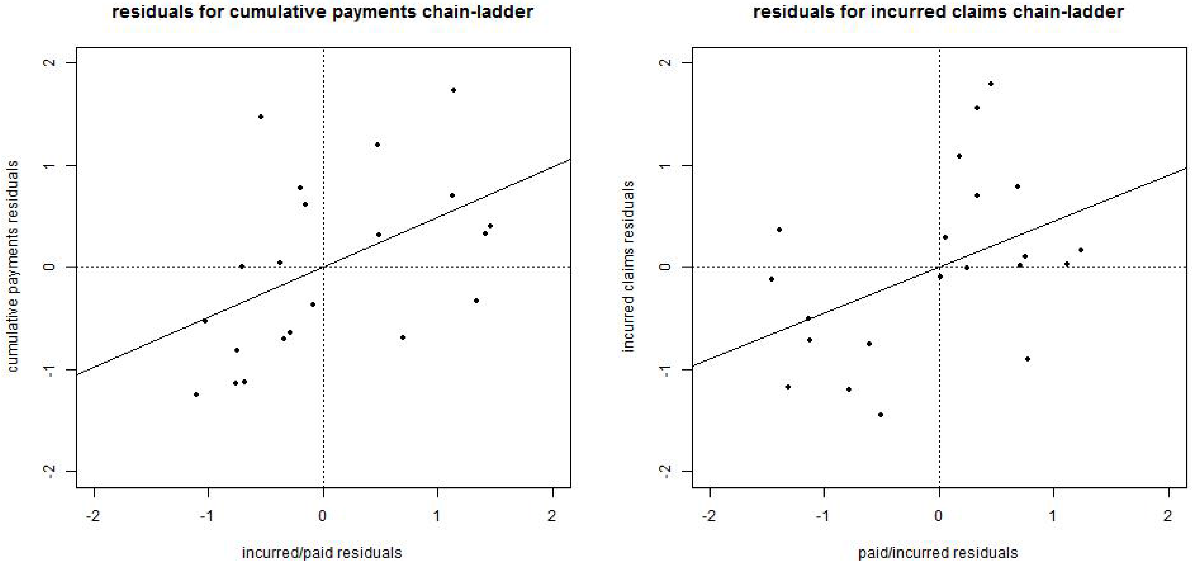
As was investigated by Quarg and Mack [1], see also Remark 2 above and Figure 1 below, we expect positive dependence between cumulative payment residuals and incurred-paid ratios (and between incurred claims residuals and paid-incurred ratios). This will be reflected by a covariance matrix choice Σ that does not have diagonal form Equation (19) but a general off-diagonal matrix A in Equation (8) such that the Schur complements are positive definite (see Assumption 5). In this case, the best predictors are provided by Theorem 4. They do not have a simple form (though their calculation is straightforward using matrix algebra). We will compare these predictors to the Munich chain-ladder predictors Equation (15) which are non-optimal in our context (see Theorem 3).
7. Example
We provide an explicit example which is based on the original data of Quarg and Mack [1], the data is provided in the Appendix A. We calculate for this data set Hertig’s chain-ladder (HCL) reserves according to Equations (18) and (21), the reserves in the modified Munich chain-ladder (mMCL) method of Theorem 4 and the (non-optimal) log-normal Munich chain-ladder (LN–MCL) reserves Equation (15) (according to Assumption 4). These reserves are based on the Bayesian multivariate log-normal framework of Assumption 5 with log-link . For comparison purposes, we also provide the classical chain-ladder (CL) reserves together with the Quarg and Mack Munich chain-ladder reserves (QM–MCL); these two latter methods differ from our results because of the different variance assumption in Assumption 1. In order to have comparability between the different approaches, we choose non-informative priors in the former Bayesian methods, see also Equations (20) and (19).
First, we need to estimate the parameters in the log-normal model of Assumption 5. For and , we choose the sample standard deviations of the observed log-link ratios and , , with the usual exponential extrapolation for the last period . Using these sample estimators, we calculate the posterior means and using Corollary 3 under choice . In the non-informative prior limit, these posterior means are given by Equation (21) (and similarly for incurred claims). This then allows one to calculate Hertig’s chain-ladder parameters and , see Equation (21). These parameters are provided in Table 1. Note that these chain-ladder factors differ from the ones in the classical chain-ladder model because of the different variance assumptions.

Table 1.
Sample standard deviations and ; posterior means and obtained from Corollary 3, see also Equation (21); and Hertig’s chain-ladder estimates and according to Equation (21).
| a.y. i/d.y. j | 0 | 1 | 2 | 3 | 4 | 5 | 6 |
|---|---|---|---|---|---|---|---|
| 7.2195 | 0.9163 | 0.1203 | 0.0296 | 0.0216 | 0.0205 | 0.0137 | |
| 0.4972 | 0.1600 | 0.0515 | 0.0069 | 0.0036 | 0.0101 | 0.0036 | |
| 1,573 | 2.5376 | 1.1296 | 1.0301 | 1.0219 | 1.0208 | 1.0138 | |
| 7.8404 | 0.5151 | 0.0137 | 0.0003 | 0.0115 | −0.0090 | −0.0037 | |
| 0.5182 | 0.1503 | 0.0406 | 0.0146 | 0.0022 | 0.0180 | 0.0022 | |
| 2,963 | 1.6959 | 1.0148 | 1.0004 | 1.0116 | 0.9912 | 0.9963 |
Using these parameters, we calculate the HCL reserves (prediction minus the last observed cumulative payments at time J), and for comparison purposes we provide the classical CL reserves. These results are provided in Table 2. The main observation is that there are quite substantial differences between the HCL reserves from cumulative payments of 6,205 and the HCL reserves from incurred claims of 7,730, see Table 2. This also holds true for the classical CL reserves 5,938 versus 7,503. This gap mainly comes from the last accident year because incurred claims observation is comparably high. We also note that the HCL reserves are more conservative than the classical CL ones. This mainly comes from the variance correction that enters the mean of log-normal random variables, see Equation (21).
To bridge this gap between the cumulative payments and the incurred claims methods we study the other reserving methods. We start with the LN–MCL method under the log-normal assumptions of Assumption 4. First we determine the correlation parameters. We use the estimators of Section 3.1.2 in [1] with changed variance functions. This provides estimates and . Note that this exactly corresponds to the positive linear dependence illustrated in Figure 1; Quarg and Mack [1] obtain under their (changed) variance assumption 64% and 44%, respectively, which is in line with our findings. Using these estimates we can then calculate the reserves in our LN–MCL method and in Quarg-Mack’s QM–MCL method. The results are provided in Table 2. We observe that the gap between the cumulative payments reserves of 6,729 and the incurred claims reserves of 7,140 becomes more narrow due to the correction factors. The same holds true for QM–MCL with reserves 6,847 and 7,120, respectively. Moreover, both models LN–MCL and QM–MCL provide rather close results, though their model assumptions differ in the variance assumption.
Table 2.
Resulting reserves from the Hertig’s chain-ladder (HCL) method based on paid and incurred; from the log-normal Munich chain-ladder (LN–MCL) method based on paid and incurred; from the modified Munich chain-ladder (mMCL) paid method; the classical chain-ladder (CL) method based on paid and incurred (inc.); and the Quarg and Mack Munich chain-ladder (QM–MCL) method paid and incurred.
| a.y. i | HCL | LN-MCL | mMCL | CL | QM-MCL | ||||
|---|---|---|---|---|---|---|---|---|---|
| paid | inc. | paid | inc. | paid | paid | inc. | paid | inc. | |
| 1 | 32 | 97 | 35 | 95 | 16 | 32 | 97 | 35 | 96 |
| 2 | 157 | 92 | 92 | 147 | 115 | 158 | 88 | 103 | 135 |
| 3 | 337 | 286 | 262 | 346 | 375 | 332 | 276 | 269 | 326 |
| 4 | 416 | 201 | 289 | 330 | 382 | 408 | 191 | 289 | 302 |
| 5 | 925 | 459 | 656 | 688 | 906 | 924 | 466 | 646 | 655 |
| 6 | 4,339 | 6,594 | 5,395 | 5,534 | 5,130 | 4,084 | 6,385 | 5,505 | 5,606 |
| total | 6’205 | 7’730 | 6’729 | 7’140 | 6’924 | 5’938 | 7’503 | 6’847 | 7’120 |
Figure 1.
(lhs) Incurred-paid residuals obtained from , see Remark 2, versus claims payments residuals obtained from , straight line has slope ; (rhs) paid-incurred residuals obtained from versus incurred claims residuals obtained from , straight line has slope .
Figure 1.
(lhs) Incurred-paid residuals obtained from , see Remark 2, versus claims payments residuals obtained from , straight line has slope ; (rhs) paid-incurred residuals obtained from versus incurred claims residuals obtained from , straight line has slope .

Finally, we study the modified Munich chain-ladder method mMCL of Assumption 5, see Theorem 4. We therefore need to specify the off-diagonal matrix , see Equation (8). A first idea to calibrate this matrix A is to use correlation estimate from the LN-MCL method. A crude approximation using Theorem 3 provides
From this, we see that in our numerical example we need comparatively high correlations, for instance, would be in line with . The difficulty with this choice is that the resulting matrix Σ of type Equation (8) is not positive definite. Therefore, we need to choose smaller correlations. We do the following choice for all
and 0% otherwise. This provides a positive definite choice for Σ of type Equation (8) in our example. This choice means that we can learn from incurred claims observations (which relate to residuals ) for cumulative payments observations with development lags , but no other conclusions can be drawn from other observations. Note that, in this example, we only use correlation choices Equation (22), but no similar choice for is done. The reason is that if we choose positive correlations for the latter, in general, Σ is not positive definite. This shows that requirement Equation (8) is rather restrictive and we expect that data usually does not satisfy Assumption 1, because both plots in Figure 1 show a positive slope.
The resulting mMCL reserves
according to Theorem 4, are provided in Table 2. Correlation choice Equation (22) means that we learn from incurred claims, which are above average for accident year . This substantially increases the mMCL reserves based on cumulative payments to 6’924. Note that we do not provide the values for incurred claims: positive definiteness of Σ restricts (under Equation (22)) which implies that we obtain almost identical values to the HCL incurred reserves for .
Finally, we analyze the prediction uncertainty measured by the square-rooted conditional mean square error of prediction. The results are provided in Table 3.
The prediction uncertainties of the HCL reserves and of the mMCL reserves were calculated according to Theorem 4. For the former (HCL reserves), we simply need to set . We see that the uncertainties in the modified version for cumulative payments are reduced from 1’249 to 1’208 because correlations Equation (22) imply that we can learn from incurred claims for cumulative payments. For incurred claims, they remain (almost) invariant because of choices for .
We can now calculate the prediction uncertainty for the LN–MCL method (which is still an open problem). Within Assumption 5, we know that the mMCL predictor is optimal, therefore, we obtain prediction uncertainty for the LN–MCL method
and similarly for incurred claims. The second term in Equation (23) is the approximation error because the LN–MCL predictor is non-optimal within Assumption 5.
Table 3.
Resulting reserves and square-rooted conditional mean square error of prediction of the different chain-ladder methods. * is calculated from Equation (23).
| Reserves | msep1/2 | |
|---|---|---|
| Hertig’s chain-ladder HCL paid | 6,205 | 1,249 |
| Hertig’s chain-ladder HCL incurred | 7,730 | 1,565 |
| log-normal Munich chain-ladder LN–MCL paid | 6,729 | 1,224* |
| log-normal Munich chain-ladder LN–MCL incurred | 7,140 | 1,673* |
| modified Munich chain-ladder mMCL paid | 6,924 | 1,208 |
| modified Munich chain-ladder mMCL incurred | 7,730 | 1,565 |
| classical chain-ladder CL paid | 5,938 | 994 |
| classical chain-ladder CL incurred | 7,503 | 995 |
| Quarg-Mack Munich chain-ladder QM–MCL paid | 6,847 | n/a |
| Quarg-Mack Munich chain-ladder QM–MCL incurred | 7,120 | n/a |
To resume, the modified Munich chain-ladder method for cumulative payments and under assumption Equation (8) provides in our example, claims reserves that are between the HCL paid and the HCL incurred reserves (as requested). Moreover, it provides the smallest prediction uncertainty among the methods based on multivariate normal distributions. This is because, in contrast to the HCL paid and HCL incurred methods, it simultaneously considers the entire information , and because there is no bias (approximation error) compared LN–MCL paid and LN–MCL incurred. These conclusions are always based on the validity of Assumption 5 which is the weakness of the method because real data typically requires different covariance matrix choices than Equation (8).
8. Conclusions
We have studied the Munich chain-ladder axioms of Quarg and Mack [1] under the moment assumptions of Assumption 1. In a multivariate log-normal modeling framework, this provides rather restrictive covariance matrix Σ requirements, see Equation (8), so that Assumption 1 is simultaneously fulfilled for cumulative payments and incurred claims. For instance, a reasonable choice of Σ for the data of Quarg and Mack [1] will differ from structure Equation (8), see Section 7 where a simultaneous choice of Equation (22) for cumulative payments and a similar choice for incurred claims would lead to a covariance matrix Σ that is not positive definite.
If Equation (8) holds, then there exists a consistent Munich chain-ladder framework, see Assumption 3, for which we can analyze claims reserves and their prediction uncertainty, see Theorem 4. Moreover, the Munich chain-ladder predictor is non-optimal in this framework, see Theorem 2, and the approximation error is provided in Theorem 3.
Author Contributions
Both authors have contributed to this document to a similar extent.
Conflicts of Interest
The authors declare no conflict of interest.
Appendix
A. Data of Quarg and Mack [1]
Table A1.
Observed cumulative payments , , source Quarg and Mack [1].
| a.y. i/d.y. j | 0 | 1 | 2 | 3 | 4 | 5 | 6 |
|---|---|---|---|---|---|---|---|
| 0 | 576 | 1,804 | 1,970 | 2,024 | 2,074 | 2,102 | 2,131 |
| 1 | 866 | 1,948 | 2,162 | 2,232 | 2,284 | 2,348 | |
| 2 | 1,412 | 3,758 | 4,252 | 4,416 | 4,494 | ||
| 3 | 2,286 | 5,292 | 5,724 | 5,850 | |||
| 4 | 1,868 | 3,778 | 4,648 | ||||
| 5 | 1,442 | 4,010 | |||||
| 6 | 2,044 |
Table A2.
Observed incurred claims , , source Quarg and Mack [1].
| a.y. i/d.y. j | 0 | 1 | 2 | 3 | 4 | 5 | 6 |
|---|---|---|---|---|---|---|---|
| 0 | 978 | 2,104 | 2,134 | 2,144 | 2,174 | 2,182 | 2’174 |
| 1 | 1,844 | 2,552 | 2,466 | 2,480 | 2,508 | 2,454 | |
| 2 | 2,904 | 4,354 | 4,698 | 4,600 | 4,644 | ||
| 3 | 3,502 | 5,958 | 6,070 | 6,142 | |||
| 4 | 2,812 | 4,882 | 4,852 | ||||
| 5 | 2,642 | 4,406 | |||||
| 6 | 5,022 |
B. Inverse Matrix Σ[1]
Consider the matrix
Set
The inverse matrix of is given by
References
- G. Quarg, and T. Mack. “Munich chain ladder.” Blätter DGVFM XXVI (2004): 597–630. [Google Scholar] [CrossRef]
- H. Liu, and R. Verrall. “Bootstrap estimation of the predictive distributions of reserves using paid and incurred claims.” Variance 4/2 (2010): 121–135. [Google Scholar]
- M. Merz, and M.V. Wüthrich. “A credibility approach to the Munich chain-ladder method.” Blätter DGVFM XXVII (2006): 619–628. [Google Scholar] [CrossRef]
- R.A. Johnson, and D.W. Wichern. Applied Multivariate Statistical Analysis, 2nd ed. Upper Saddle River, NJ, USA: Prentice-Hall, 1988. [Google Scholar]
- S. Boyd, and L. Vandenberghe. Convex Optimization. Cambridge, UK: Cambridge University Press, 2004. [Google Scholar]
- M.V. Wüthrich, and M. Merz. “Stochastic claims reserving manual: Advances in dynamic modeling.” Available online: http://papers.ssrn.com/sol3/papers.cfm?abstract-id=2649057 (accessed on 21 December 2015).
- J. Hertig. “A statistical approach to the IBNR-reserves in marine insurance.” ASTIN Bull. 15/2 (1985): 171–183. [Google Scholar] [CrossRef]
© 2015 by the authors; licensee MDPI, Basel, Switzerland. This article is an open access article distributed under the terms and conditions of the Creative Commons Attribution license (http://creativecommons.org/licenses/by/4.0/).
Share and Cite
MDPI and ACS Style
Merz, M.; Wüthrich, M.V. Modified Munich Chain-Ladder Method. Risks 2015, 3, 624-646. https://doi.org/10.3390/risks3040624
AMA Style
Merz M, Wüthrich MV. Modified Munich Chain-Ladder Method. Risks. 2015; 3(4):624-646. https://doi.org/10.3390/risks3040624
Chicago/Turabian StyleMerz, Michael, and Mario V. Wüthrich. 2015. "Modified Munich Chain-Ladder Method" Risks 3, no. 4: 624-646. https://doi.org/10.3390/risks3040624