1. Introduction and Motivation
Long-term care insurance (LTCI) products deserve, in the framework of insurances of the person, special attention. Actually, on the one hand, LTCI provides benefits of remarkable interest in the current demographic and social scenario, and on the other, LTCI covers are “difficult” products. We note in particular the following aspects (see, e.g., [
1]).
In many countries, the shares of the elderly population are rapidly growing because of increasing life expectancy and low fertility rates.
Household sizes are progressively reducing, and this causes a lack of assistance and care services provided to old members of the family inside the family itself.
LTCI covers are rather recent products, and consequently, experience data are scanty; pricing and reserving problems then arise because of difficulties in the choice of appropriate technical bases.
Significant safety loadings may be charged to policyholders, because of uncertainty in the biometric assumptions.
High premiums (in particular due to safety loadings) constitute an obstacle to the diffusion of these products and especially stand-alone LTCI covers, which only provide “protection”.
The remarkable interest in LTCI products has stimulated many scientific and technical contributions to this topic. The reader can refer to Chapter 3 of [
1] for a compact description of the main LTCI products and the related packaging possibilities; see also the references therein. We note, in particular, that combining a life annuity and LTCI benefits can provide the annuitant with protection against the risk of outliving his/her assets available at retirement and, at the same time, against the extra risk originated by senescent disability. This subject is extensively dealt with in the book by [
2]. Other interesting contributions on packaging life annuities and LTCI benefits have been provided, in particular by [
3,
4,
5,
6]. In [
7], life annuities combined with LTCI benefits are analyzed in the framework of guarantee structures in life annuity products. Including an LTCI cover, as a rider benefit, into a whole life insurance policy is discussed, for example, by [
8].
As regards actuarial modeling issues, we cite the book by [
9], where premium and reserve calculations for disability and LTCI benefits are described in the framework of Markov (and semi-Markov) models, in both a time-continuous and a time-discrete context.
It is worth noting some critical issues in the choice of an appropriate stochastic model for LTCI covers (as well as for combined products also including lifetime-related benefits). The following points should be carefully considered:
whether to allow or not for the inception-dependence of some probabilities (namely, the probability of recovery (see also Point 2 below) and the probability of death), which in the case of dependence are functions of both the insured’s current age and the time elapsed since the LTC claim (that is, the senescent disability inception);
whether to take into account or not the possibility of recovery from LTC states.
The following aspects should in particular be stressed, as they can suggest appropriate modeling choices, consistent with data availability.
Inception dependence calls for a semi-Markov setting (instead of a Markov setting). Further, detailed statistical evidence is needed in order to estimate probabilities depending on both the attained age and the time elapsed since disability inception. Conversely, adopting a Markov model can lead to biased evaluations for short-duration disability. However, senescent disability is typically chronic, or anyway long lasting, so that significant biases should not be caused by a Markov setting. Further, it is interesting to note that a semi-Markov dependence structure can also be implemented within a Markov setting, via an appropriate redefinition of the state space; an interesting example is provided by the so-called Dutch model for disability annuities, described by [
10].
The prevailing chronic character of the LTC disability suggests disregarding the recovery possibility. Indeed, the frequency of recovery is particularly low if the benefit eligibility is restricted to severe LTC conditions. Of course, this results in a simpler Markov model.
Recent literature witnesses various choices as regards the modeling issues mentioned above. Semi-Markov models, and hence, inception-dependent probabilities, have been used in particular by [
11,
12]. Experience data, which can underpin inception-select probabilities (and, in particular, inception-select mortality), are presented and discussed by [
13]. Conversely, Markov models have been adopted by [
3,
8,
14,
15].
Various models for representing the extra-mortality of disabled people, either allowing for inception-dependence or not, are reviewed by [
16].
While managing a portfolio of policies in the area of the insurances of the person, the insurer takes several risks, in particular biometric risks, i.e., related to mortality, disability, etc. For each risk, various components can be recognized and, in particular, the risk of random fluctuations (of mortality, disability, etc.) around the relevant expected values and the risk of systematic deviations from the expected values. As is well known, the former is diversifiable via pooling, whereas the latter is undiversifiable via pooling, and its impact is larger when the portfolio size is larger.
The risk of systematic deviations is frequently originated by uncertainty in the technical bases (i.e., assumptions regarding mortality, disability, etc., and the related trends).
This paper focuses on the impact of uncertainty in the technical bases, which must be adopted when pricing and reserving for LTCI policies. A sensitivity analysis will be performed, in order to assess the change in expected present values of benefits when changing:
the assumptions about senescent disability, in terms of the probability of entering the LTC state(s);
the age-pattern of mortality of people in LTC state(s).
The sensitivity analysis will be performed starting from the biometric assumptions proposed by [
17,
18]. Both the LTC stand-alone cover and some LTC combined products will be addressed, and the advantages provided by packaging LTC benefits together with lifetime-related benefits (
i.e., conventional life annuities and death benefits) will be checked.
The remainder of the paper is organized as follows. In
Section 2, we describe the basic long-term care insurance products, whereas
Section 3 focuses on a simple actuarial model for premium calculation. Formulae for premiums and numerical examples are provided in
Section 4. The sensitivity analysis is the object of
Section 5, which constitutes the core of the paper. Some final remarks in
Section 6 conclude the paper.
We stress that the paper does not aim to provide a methodological innovation. Indeed, the theoretical framework is a standard one. Conversely, the paper, adopting an empirical approach, presents and discusses numerical results, which can help in finding appropriate product designs, aiming to mitigate the impact of risks arising from table or parameter uncertainty.
1 2. Long-Term Care Insurance Products
Long-term care insurance (LTCI) provides the insured with financial support, while he/she needs nursing and/or medical care because of chronic (or long-lasting) conditions or ailments.
Several types of benefits can be provided (in particular: fixed-amount annuities, care expense reimbursement). The benefit trigger is usually given either by claiming for nursing and/or medical assistance (together with a sanitary ascertainment) or by assessment of the individual disability, according to some predefined metrics, e.g., the Activities of Daily Living (ADL) scale or the Instrumental Activities of Daily Living (IADL) scale; see, for example, [
1] and the references therein. We note that, in different insurance markets, different criteria for the LTCI benefit eligibility are adopted. This can complicate the problem of choosing, for a given LTCI product, reliable statistical data concerning the senescent disablement and mortality of disabled people.
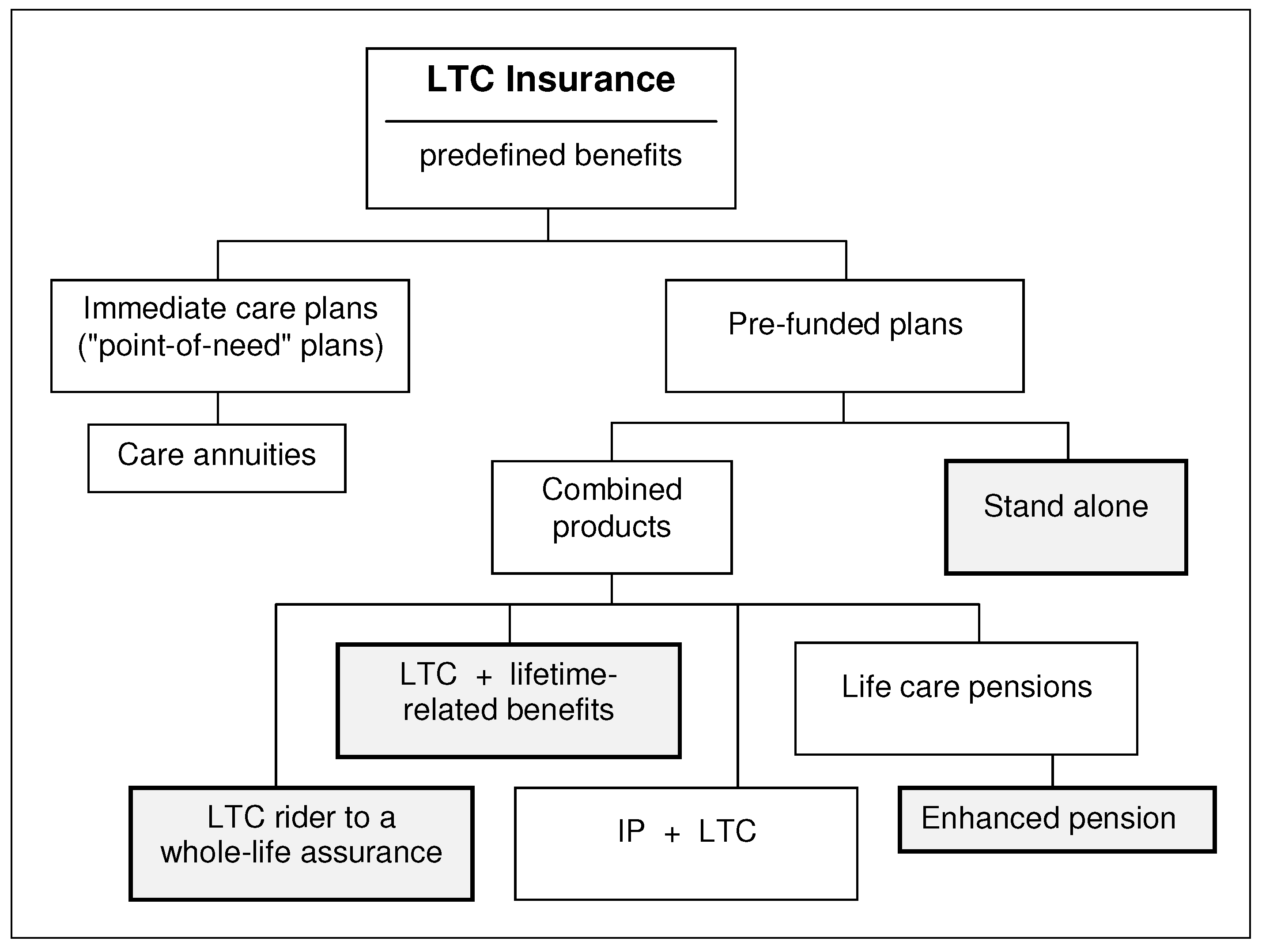
2.1. LTCI Products: A Classification
Long-term care insurance products can be classified as follows:
In what follows, we only address LTCI products that provide benefits with a predefined amount.
2.2. Fixed-Amount and Degree-Related Benefits
A classification of LTCI products that pay out benefits with a predefined amount is proposed in
Figure 1; the shaded boxes refer to the insurance covers considered in the sensitivity analysis.
Immediate care plans, or
care annuities, relate to individuals already affected by severe disability (that is, in “point of need”), and then consist of:
the payment of a single premium;
an immediate life annuity, whose annual benefit may be graded according to the disability severity.
Hence, care annuities are aimed at seriously impaired individuals, in particular persons who have already started to incur LTC costs. The premium calculation is based on assumptions of short life expectancy. However, the insurer may limit the individual longevity risk by offering a limited term annuity, namely a temporary life annuity.
Pre-funded plans consist of:
the accumulation phase, during which periodic premiums are (usually) paid; as an alternative, a single premium can be paid (of course, while the insured is in the healthy state);
the payout period, during which LTC benefits (usually consisting of a life annuity) are paid in the case of LTC need.
Several products belong to the class of pre-funded plans. A stand-alone LTC cover provides an annuity benefit, possibly graded according to an ADL or IADL score. This cover can be financed by a single premium, by temporary periodic premiums or lifelong periodic premiums. Of course, premiums are waived in the case of an LTC claim. This insurance product only provides a “risk cover”, as there is, of course, no certainty in future LTC need and the consequent payment of benefits.
A number of combined products have been designed, mainly aiming at reducing the relative weight of the risk component by introducing a “saving” component, or by adding the LTC benefits to an insurance product with a significant saving component. Some examples follow.
LTC benefits can be added as a rider to a whole-life assurance policy (and, hence, can constitute an incentive against surrendering the policy). For example, a monthly benefit of, say, 2% of the sum assured is paid in the case of an LTC claim, for 50 months at most. The death benefit is consequently reduced and disappears if all of the 50 monthly benefits are paid. Thus, the (temporary) LTC annuity benefit is simply given by an acceleration of (part of) the death benefit. The LTC cover can be complemented by an additional deferred LTC annuity (financed by an appropriate premium increase), which will start immediately after the possible exhaustion of the sum assured (that is, if the LTC claim lasts for more than 50 months) and will terminate at the insured’s death.
An insurance package can include LTC benefits combined with
lifetime-related benefits,
i.e., benefits only depending on the insured’s survival and death. For example, the following benefits can be packaged:
a lifelong LTC annuity (from the LTC claim on);
a deferred life annuity (e.g., from age 80), while the insured is not in the LTC disability state;
a lump sum benefit on death, which can alternatively be given by:
- (a)
a fixed amount, stated in the policy;
- (b)
the difference (if positive) between a stated amount and the amount paid as Benefit 1 and/or Benefit 2.
We note that Item 2,
i.e., the old-age deferred life annuity, provides protection against the individual longevity risk to people in good health conditions and then constitutes an ALDA (advanced life delayed annuity), proposed by [
20].
Life care pensions (also called life care annuities) are life annuity products in which the LTC benefit is defined in terms of an uplift with respect to the basic pension b. In particular, the enhanced pension is a life care pension in which the uplift is financed by a reduction (with respect to the basic pension b) of the benefit paid while the policyholder is healthy. Thus, the reduced benefit is paid out as long as the retiree is healthy, while the uplifted benefit will be paid in the case of an LTC claim (of course, ).
Finally, a
lifelong disability cover can include:
3. The Model
In this section, we first describe multi-state models that can be adopted to represent “states” and “transitions” related to an LTCI cover. We then introduce the biometric functions that are needed to assign a stochastic structure to the multi-state model chosen for the following calculations. Actuarial values (i.e., expected present values) are then defined, and finally, technical bases are addressed.
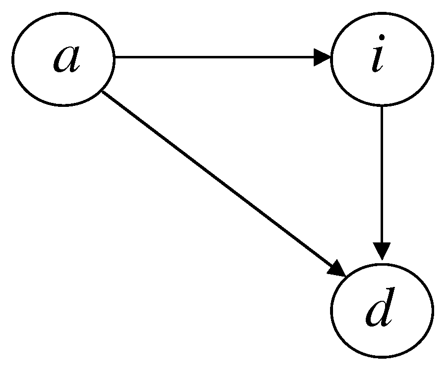
3.1. Multi-State Models for LTCI
The multi-state model we have adopted for the empirical analysis simply consists of three states and three possible transitions (see
Figure 2). The states are:
a = active (i.e., healthy);
i = incapacitated, or invalid (i.e., in the LTC state);
d = died;
and the transitions are as follows:
= disablement (i.e., entering the LTC state);
= death from the active state;
= death from the LTC state.
Hence, just one LTC state has been considered, from which recovery is not allowed. See
Section 1 for comments about this choice.
Of course, more complex multi-state models can be considered, for example including two or more disability states (corresponding to more or less severe health conditions) to represent a degree-related benefit structure.
For a more detailed presentation of multi-state models for LTCI, the reader can refer to [
1] and [
9], where a time-continuous context is considered.
3.2. Biometric Functions
We refer to the three-state model shown in
Figure 2. A Markov setting has been chosen; thus, no inception-dependence has been allowed for (for comments on this choice, see
Section 1).
We define, for a healthy individual age
x, the following one-year probabilities (the traditional actuarial notation has been adopted):
probability of being healthy at age ;
probability of being an invalid at age ;
probability of dying before age from state a;
probability of dying before age from state i;
probability of dying before age ;
probability of becoming an invalid (disablement) before age .
For an invalid individual (
i.e., an individual in the state of LTC) of age
x, we consider the following one-year probabilities:
The following relations obviously hold:
The (usual) approximation:
has been assumed; in its turn, Equation (
5) implies:
From the one-year probabilities, the following multi-year probabilities can be immediately derived:
Of course, we have: , and .
3.3. Actuarial Values
Let
v denote the annual discount factor. We define the following actuarial values (
i.e., expected present values). The usual actuarial notation is adopted.
Actuarial value, for a healthy individual age
x (
i.e., in state
a), of a life annuity providing a benefit of one monetary unit per annum, payable at the policy anniversaries, while the individual is disabled (
i.e., in state
i):
Actuarial value, for a disabled individual age
, of a life annuity providing a benefit of one monetary unit per annum, payable at the policy anniversaries, while the individual is disabled:
Actuarial value, for a disabled individual age
, of a temporary life annuity providing a benefit of one monetary unit per annum, payable at the policy anniversaries, while the individual is disabled:
Actuarial value, for a healthy individual age
x, of a life annuity of one monetary unit per annum, payable at the policy anniversaries, while the individual is healthy:
Actuarial value, for a healthy individual age
x, of a temporary life annuity of one monetary unit per annum, payable at the policy anniversaries, while the individual is healthy:
Actuarial value, for a healthy individual age
x, of a deferred life annuity of one monetary unit per annum, payable at the policy anniversaries, while the individual is healthy:
3.4. Technical Bases
We assume that:
is given by the first Heligman–Pollard law;
is expressed by a specific parametric law;
(that is, an additive extra-mortality model is adopted).
The first Heligman–Pollard law is defined as follows:
(see [
21]).
The parameters have been assigned the numerical values given in
Table 1. Some corresponding markers are shown in
Table 2, in particular:
the (remaining) expected lifetime, , at various ages x;
the Lexis point, , i.e., the (old) age with the maximum probability of death for a newborn;
the one-year probability of death, , at various ages x.
We note that the parameter values have been chosen so that the resulting age pattern of mortality fits a projected market life table (that is, describing the mortality of healthy insured people), which incorporates a forecast of future mortality improvements, as can be argued looking at the expected lifetimes and the Lexis point (see
Table 2).
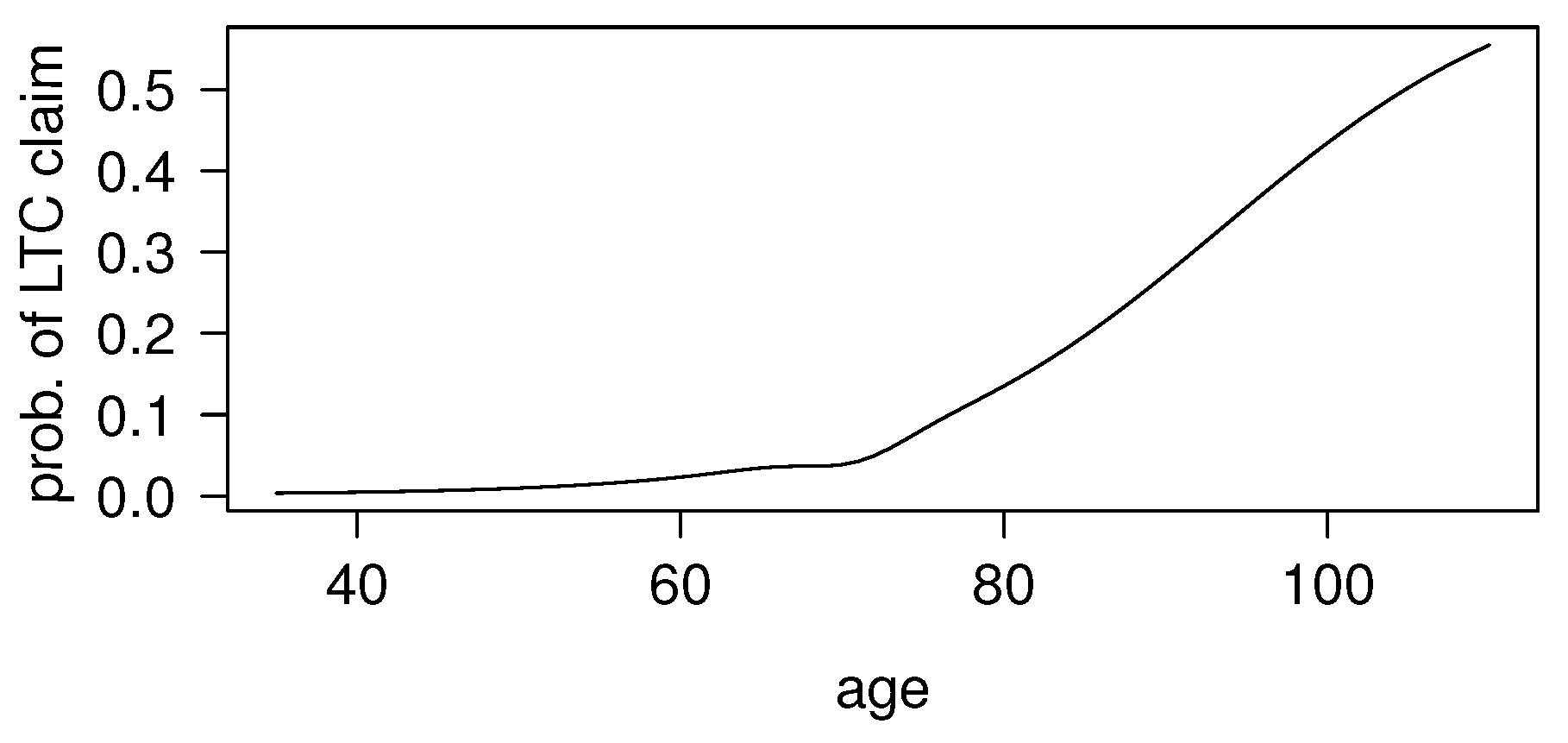
The assumption proposed by [
17] has been adopted for the one-year probability of disablement, that is:
The relevant parameters are given in
Table 3. The function
(for males) is plotted in
Figure 3.
An additive extra-mortality model has been assumed to represent the mortality of disabled people. As suggested by [
17], we have adopted the following formula:
with:
As regards the parameters and the related values, we note what follows.
Parameter
k expresses the LTC severity category, according to the OPCS scale (see [
22]); in particular:
denotes a less severe LTC states, with no impact on mortality;
denotes a more severe LTC states, implying extra-mortality;
In the following calculations, we have assumed , that is a severe LTC state (so that the possibility of recovery can be disregarded). Hence, for all x.
According to [
18], we have set
, as we have assumed
(that is, the mortality of insured healthy people).
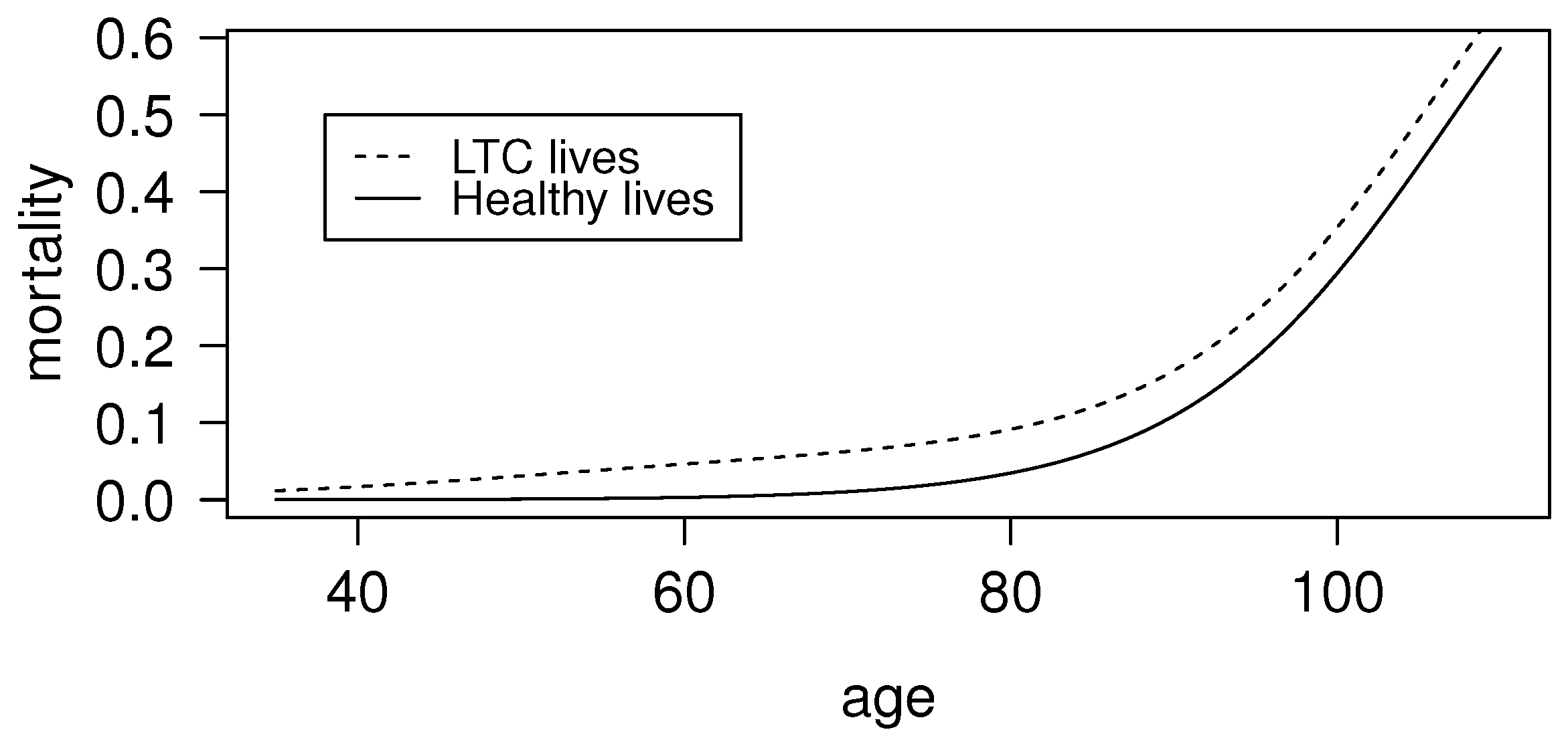
From the previous assumptions, it follows:
The age patterns of mortality for healthy people (
i.e., the function
) and for disabled people (
i.e., the function
) are plotted in
Figure 4. The underlying assumptions are given by the Heligman–Pollard law (see Equation (
16) and
Table 1) and the additive extra-mortality model (see Equation (
18) and Equation (
20)).
In all of the numerical calculations in
Section 4, we have assumed the interest rate to be
, and hence,
; the biometric assumptions refer to males.
4. Premiums
We consider the following LTCI products (see
Section 2.2 for the definitions of the relevant benefits):
Product P1: stand-alone LTC cover;
Product P2: LTC acceleration benefit in a whole-life assurance;
Product P3: LTC insurance package, including a deferred life annuity and a death benefit; in particular:
Product P4: enhanced pension.
Some comments follow, concerning the choice of the products to be analyzed.
First, we note that LTCI covers that provide expense reimbursement have been excluded from our analysis. Expense-related benefits can provide a good coverage of LTC needs, but the characteristics of the related insurance products and the relevant actuarial problems significantly differ from the features of the products providing predefined benefits. Indeed, random amounts of LTC expenses imply, on the one hand, specific actuarial models and, on the other, the presence of policy conditions (i.e., fixed-percentage or fixed-amount deductible, limit amount, etc.) similar to those commonly adopted in non-life insurance. Finally, we note that the evaluation of expense-related benefits calls for an important collection of data, which, to some extent, are country specific and, hence, affected by a high degree of heterogeneity.
As regards the LTCI products providing predefined benefits, we first note that two “extreme” products have been included in the analysis, i.e., the stand-alone cover (Product P1) and the whole-life assurance with LTCI as an acceleration benefit (Product P2). While the former only aims at contributing to cover the LTC needs, the latter has an important savings component and a rather limited LTC coverage.
The two remaining products either include a life annuity component (Product P2) or are “derived” from a life annuity or pension product, thus aiming at covering the individual longevity risk.
Although other products are sold on various insurance markets, the products we are addressing represent important LTCI market shares, and at the same time, their simple structures ease the sensitivity analysis and the interpretation of the results.
According to the equivalence principle, the single premiums are given by the actuarial values of the benefits.
4.1. Product P1: LTCI as a Stand-Alone Cover
According to the notation adopted in
Section 3.3, the single premium, for an annual benefit
b payable in arrears, is given by:
and the annual level premiums by:
in the case of non-temporary or temporary premiums, respectively. Some numerical examples are shown in
Table 4.
4.2. Product P2: LTCI as an Acceleration Benefit
Refer to a whole life assurance with sum assured
C, payable at the end of the year of death. The acceleration benefit consists of a temporary LTC annuity with annual benefit
(this benefit could also be payable on a monthly basis, as mentioned in
Section 2). The single premium,
, of the whole life assurance with the LTC acceleration benefit is given by:
Conversely, the single premium for a (standard) whole life assurance is given by:
Table 5 provides some examples. We note that, for any given age
x at policy issue, the higher is
s, the lower is the single premium because of spreading the benefit over a longer period from the disability inception. In particular, if
, then the whole amount
C is paid as a lump sum, either at the end of the year of requiring LTC or at the end of the year of death. We also note that, assuming a zero interest rate, the single premium would be equal to
C (whatever the value of
s) as the payment of the benefit is sure, only the time and the cause of payment being random.
4.3. Product P3: LTCI in Life Insurance Package
Package (a) provides the following benefits (see also
Section 2.2):
a life annuity with annual benefit , deferred n years, while the individual is healthy;
an LTC annuity with annual benefit ;
a death benefit C.
The single premium,
, is given by:
Some numerical examples are provided in
Table 6.
Package (b) includes the following benefits (see also
Section 2.2):
a life annuity with annual benefit , deferred n years, while the individual is healthy;
an LTC annuity with annual benefit ;
a death benefit given by
, where:
The single premium is then given by the following expression:
where the quantity
denotes the actuarial value of the death benefit. This quantity can be split into four terms, according to possible individual stories:
The four terms refer to the following mutually-exclusive stories.
Death in healthy state before time
n:
In this case, we have: .
Death in healthy state after time
n:
Then: .
Death in LTC state, entered before time
n:
In this case: .
Death in the LTC state, entered after time
n:
In this case, we have: .
Some numerical examples are provided in
Table 7. We note that, for any age
x and any deferment
n, we find
because of the different definition of the death benefit.
4.4. Product 4: the Enhanced Pension
The single premium for a standard pension with annual benefit
b is given by:
The single premium for a pension with annual benefits
,
, respectively paid if the annuitant is either healthy or in the LTC state, is given by:
In the case of an enhanced pension, we must have:
and then:
From Equation (
35), given
, we can calculate the reduced pension
. Conversely, given
, we can find the uplifted pension
. Some numerical examples are given in
Table 8.
5. Sensitivity Analysis
In this section, we refer to the four LTCI products addressed in
Section 4 and assess the sensitivity of the single premiums with respect to the assumptions concerning the probability of disablement and the extra-mortality.
Let
denote the single premium of the LTCI product PX, with X = 1, 2, 3, according to the following assumptions:
probability of entering the LTC state (
i.e., probability of disablement)
, defined as follows:
where
is given by Equation (
17), with parameters as specified in
Table 3 for males;
extra-mortality of people in the LTC state, defined as follows:
(see Equation (
20)); it follows that the mortality of disabled people is given by:
we note that
means the absence of extra-mortality.
As regards the product P4, let denote the amount of the reduced pension that meets a given uplifted pension (for a given value of b), according to the assumptions expressed by δ and λ.
To ease the comparisons, we define for the LTCI products P1, P2 and P3 the “normalized” single premium, that is the ratio:
whereas for the product P4, with given
b and
, we define the ratio:
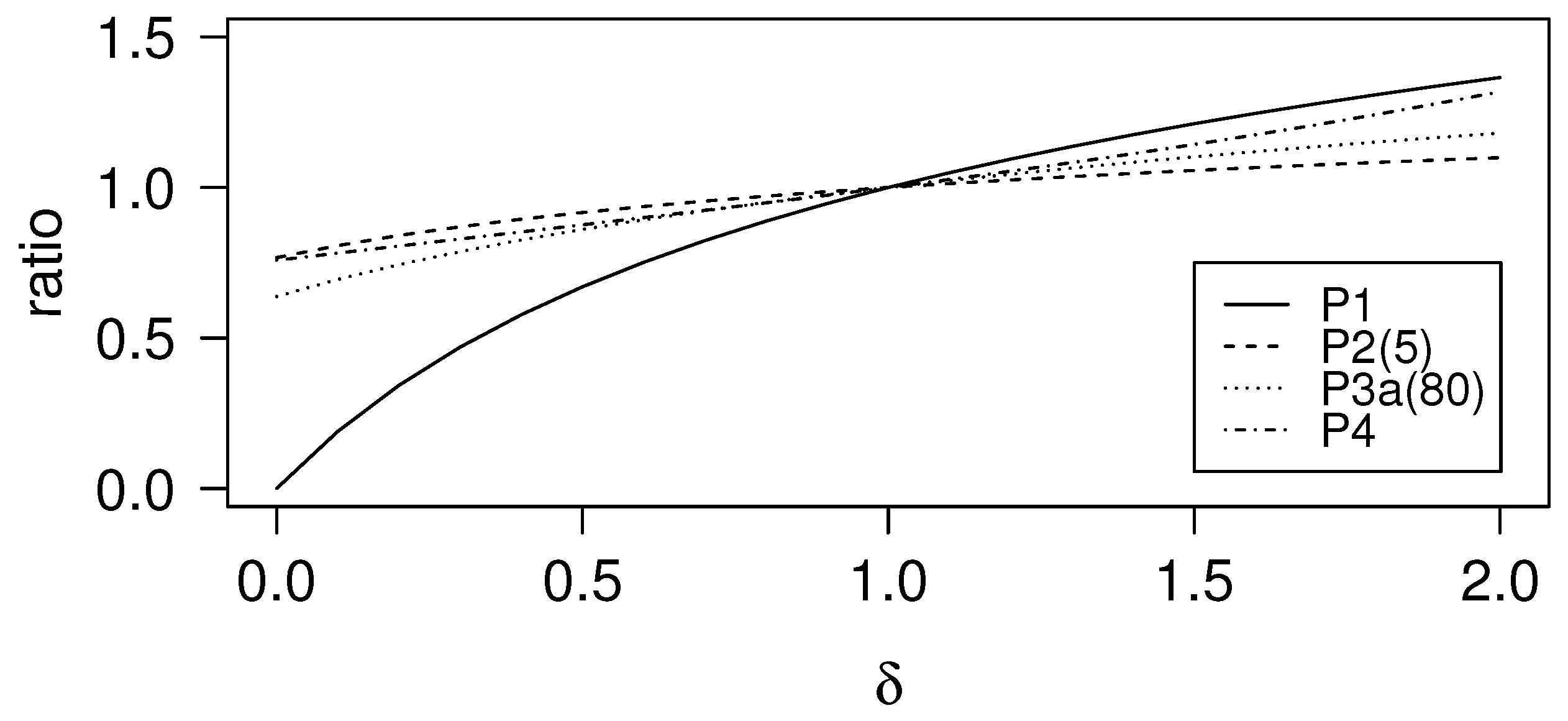
For all of the products, we first perform a “marginal” analysis, by analyzing the behavior of the functions:
to assess the sensitivity with respect to the disablement assumption (
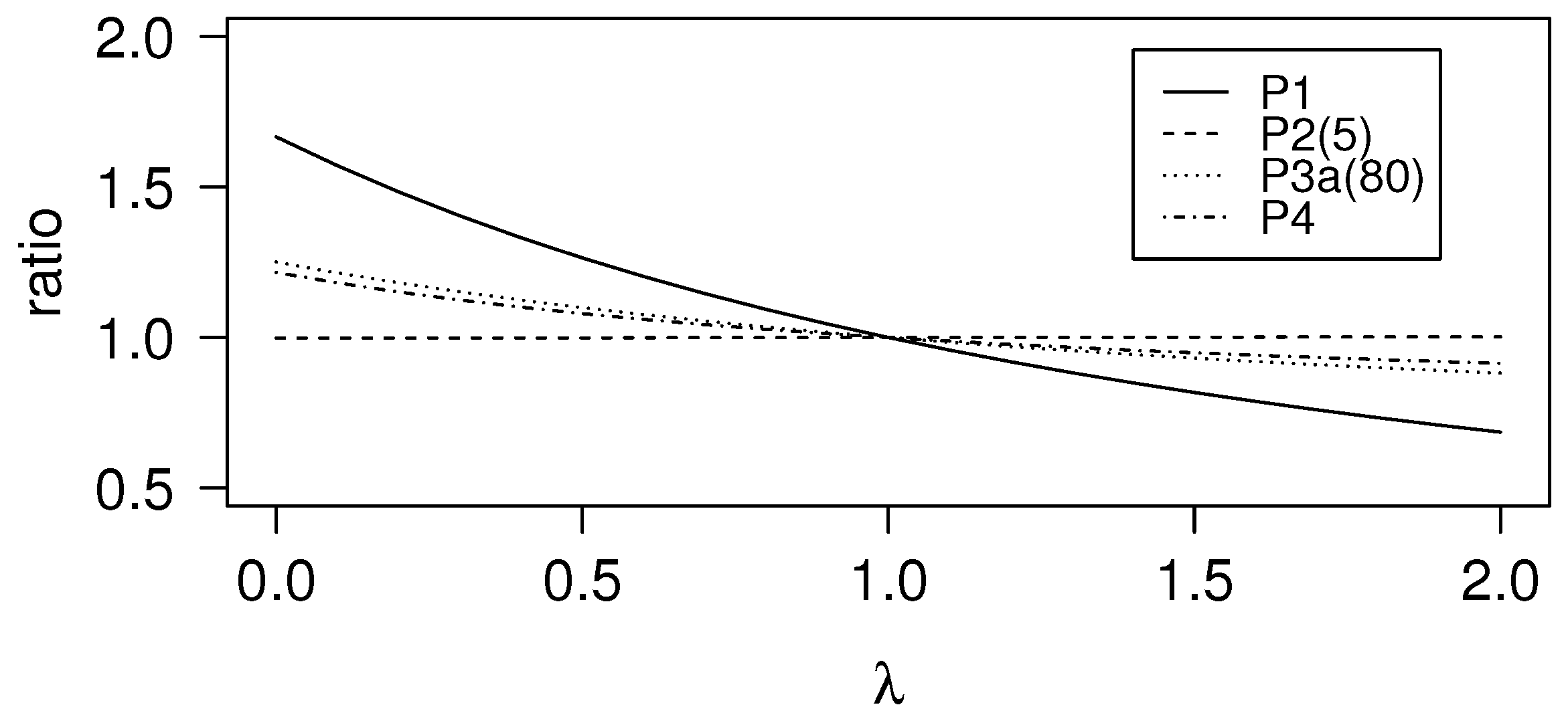
Section 5.1) and the functions:
to assess the sensitivity with respect to the mortality assumption (
Section 5.2).
Some results of a “joint” sensitivity analysis are finally presented (
Section 5.3).
The following comments may be helpful in understanding the choice of the intervals for the parameters λ and δ and the impact of parameter values other than one. First, we note that, intuitively, the actuarial values of payments linked to LTC would increase as the probability of entering into LTC increases and would reduce as the extra-mortality from the LTC state increases. If an LTC benefit is added as a rider to accelerate insurance payments in whole-life assurance, the certainty of the payment implies that the actuarial value would be less sensitive relative to a similar LTC payment that is uncertain.
As regards the numerical values of the parameter δ, we in particular note that values lower than one (say, ) can express a realistic estimate of the probability of becoming disabled, since only severe LTC states are considered to qualify the insured as eligible for LTCI benefits.
The parameter λ affects the extra-mortality of the disabled individuals. While parameter values close to two can represent a realistic estimate of the mortality of people in very severe health conditions, values lower than one lead to prudential actuarial valuations ( representing, of course, the unrealistic absence of extra-mortality).
5.1. Disablement Assumption
Some results of sensitivity analysis with respect to disablement assumption are shown in
Table 9,
Table 10,
Table 11 and
Table 12, in terms of single premiums, normalized single premiums and reduced benefit in the enhanced pension.
From the numerical results, we immediately recognize the stand-alone LTCI product,
i.e., Product P1, as the one with the highest sensitivity with respect to the disablement assumption. This (rather intuitive) result is also evident in graphical terms, as shown by
Figure 5. We note, in particular, the dramatic impact of a possible underestimation of the probability of disablement, expressed by
(even excluding non-realistic underestimations, which could be represented by, say,
).
5.2. Extra-Mortality Assumption
Some results of sensitivity analysis with respect to the extra-mortality assumption are shown in
Table 13,
Table 14,
Table 15 and
Table 16, in terms of single premiums, normalized single premiums and reduced benefit in the enhanced pension.
The numerical results show that the stand-alone LTCI product,
i.e., Product P1, is the one with the highest sensitivity also with respect to the extra-mortality assumption. See
Figure 6. We note that, as P1 provides a living benefit, a safety loading could be included in the premium by underestimating the extra-mortality of disabled people.
Conversely, the extra-mortality assumption has no impact on the premium of the whole life assurance with acceleration benefit if : indeed, in this case, the whole death benefit is paid upon the LTC claim. Further, a very low impact affects the case .
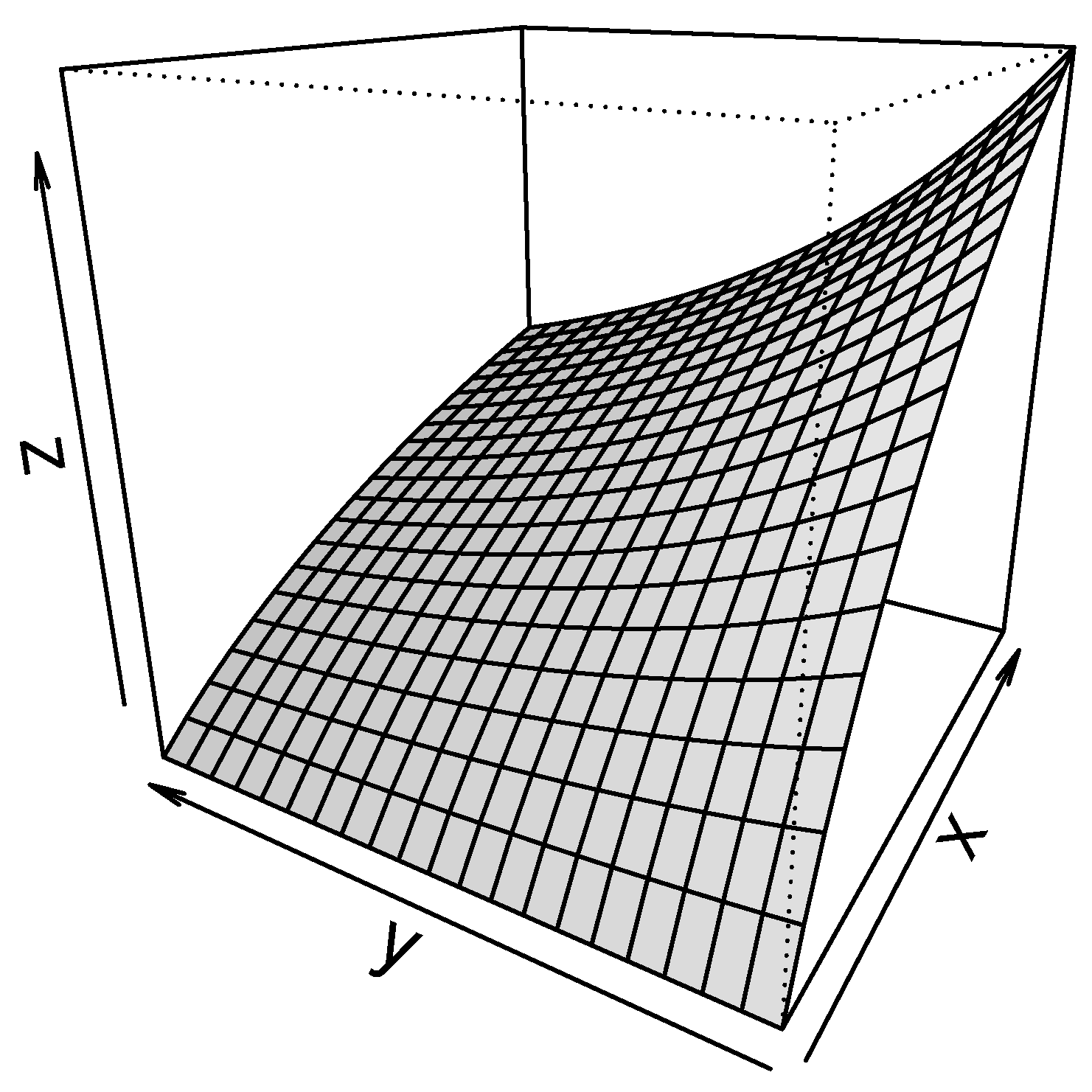
5.3. Joint Sensitivity Analysis
A joint sensitivity analysis can produce various results of practical interest. It can be performed looking, in particular, at the surface, which represents the behavior of the function:
For example,
Figure 7 shows the behavior of the function
.
For brevity, we only focus on sensitivity analysis aiming to find, for the generic product PX and a given age
x, the set of pairs
, such that:
Equation (
42) implies for Products P1, P2, P3:
We note that Equation (
43) represents an “iso-premium” line: actually, all of the pairs
that fulfill this equation lead to the same single premium.
For Product P4, Equation (
42) implies:
Hence, the graphical representation of Equations (42)–(44) provides insight into the possible offset between, for example, an overestimation of the extra-mortality and an overestimation of the probability of entering the LTC state.
The iso-premium curves plotted in
Figure 8 show this possibility with reference to Products P1 and P3a(80). We note that, thanks to the wide ranges chosen for both parameters, the possibility of offset appears effective also in the case of significant under- or over-estimation of the parameters.
6. Concluding Remarks
A numerical analysis has been carried out to assess the sensitivity of various LTCI products with respect to the basic biometric assumptions (probability of disablement and extra-mortality of disabled people).
The normalized ratio of premiums has been chosen to provide a numerical assessment of the sensitivity. It should be noted, however, that the resulting comparisons only describe the insurer’s exposure to the uncertainty risk, while they do not provide a complete picture of the sensitivities, especially because of difficulties in finding the equivalent level of coverage from the various products.
Numerical examples show, in particular, that the LTC stand-alone cover is much riskier than all of the LTC combined products that we have considered. As a consequence, the LTC stand-alone cover is a highly “absorbing” product as regards capital requirements for solvency purposes.
Combined LTCI products mainly aim at reducing the relative weight of the “risk” component by introducing a “saving” component into the product, or by adding LTC benefits to an insurance product with an important saving component.
In more general terms, in the area of health insurance a combined product can result in being profitable to the insurance company, even if one of its components is not profitable, and further, it can be less risky than one of its components, being in particular less exposed to the impact of the uncertainty risk related to the choice of technical bases.
From the client’s perspective, purchasing a combined product can be less expensive than separately purchasing all of the single components, in particular thanks to a reduction of acquisition costs charged to the policyholder, but also thanks to a possible lower total safety loading. Of course, allowing for different clients’ preferences would call for a more complex analysis, which should be defined in terms of personal wealth and health management process.


