Improving Convergence of Binomial Schemes and the Edgeworth Expansion

Abstract

Binomial trees are very popular in both theory and applications of option pricing. As they often suffer from an irregular convergence behavior, improving this is an important task. We build upon a new version of the Edgeworth expansion for lattice models to construct new and quickly converging binomial schemes with a particular application to barrier options.

1. Introduction: Convergence of Binomial Trees

Since the appearance of the pioneering work by Cox et al. (see [1]) and by Rendleman and Bartter (see [2]), the use of binomial trees in option pricing has been very popular in both application and theory. Their main advantages are that they inherit the important theoretical concepts of completeness and risk-neutral pricing while keeping the technical framework on a very low level. In particular, they can be applied without the necessity to introduce stochastic calculus.

Further, approximating option prices in the Black–Scholes model (BS model) or more advanced models with the help of a sequence of suitable binomial trees is a popular numerical method when it comes to exotic options, in particular those with American or Bermudan features.

Convergence of such a sequence of approximations to the desired option price in the BS model is ensured by constructing the corresponding binomial trees in a way such that they satisfy the (approximate) moment matching conditions of Donsker’s theorem (see, e.g., [3,4]). However, conventional sequences of binomial trees (such as the Cox–Ross–Rubinstein tree (CRR tree) or the Rendleman–Bartter tree (RB tree)) show a quite erratic convergence behavior, which is typically not monotonic in the number of periods n (i.e., the fineness of the trees) and is often referred to as the sawtooth effect.

This issue has been addressed by numerous authors, and different solutions have been offered (see, e.g., [5,6,7,8]). In order to better understand the source of the problem, as well as to be able to compare existing methods theoretically, one has to consider the asymptotics of the discrete models ([9,10]). Moreover, this information can then be used to construct advanced tree models with faster or smoother convergence (see [11,12,13]).

We will focus on the BS model in the one-dimensional setting. There, we offer a general method of constructing asymptotic expansions for lattices based on an appropriate Edgeworth expansion and discuss ways of further improving the convergence behavior for different types of options.

Edgeworth expansions have various applications in the literature, e.g., in statistics. In the context of binomial trees, the Edgeworth expansion has been applied, e.g., by Rubinstein (see [14]) to construct risk-neutral approximations for various types of distributions, however, without providing the exact convergence behavior.

In this article, we propose a new approach to analyze the asymptotic behavior of binomial trees via the introduction of the Edgeworth expansion for lattice triangular schemes. This method provides a general framework for improving the convergence of binomial trees that is not restricted to risk-neutral transition probabilities and can be easily applied to multinomial and multidimensional trees. As an application we provide an asymptotic expansion for the performance of binomial trees for barrier options and construct an extended CRR tree with an improved convergence behavior.

2. Asymptotic Analysis of Binomial Trees: Distributional Fit

Consider the one-dimensional BS model in the risk-neutral setting given by:

$$dS\left(t\right)=S\left(t\right)\left(rdt+\sigma dW\left(t\right)\right),S\left(0\right)=s_0$$

(1)

where $W\left(t\right)$ is a Brownian motion under the risk-neutral measure Q. We then construct approximating binomial trees $\left\{S_k^{\left(n\right)}\right\}$, $k=1,\cdots ,n$ via:

$$S_k^{\left(n\right)}=S_{k-1}^{\left(n\right)}{e}^{{\alpha }_n\Delta t+\sigma \sqrt{\Delta t}{\xi }_k^{\left(n\right)}},S_0^{\left(n\right)}=s_0$$

(2)

where ${\left\{{\alpha }_n\right\}}_n$ is a bounded sequence and for each $n\in \mathbb{N}$, ${\xi }_k^{\left(n\right)}$, $k=1,\cdots ,n$ are i.i.d random variables taking on values of one and $-1$ with probabilities $p_n$ and $1-p_n$, respectively.

The convergence behavior of the binomial trees above can be controlled with an appropriate selection of values ${\alpha }_n$ and $p_n$. However, in order to ensure weak convergence, the mean and variance of the one-period log returns of the discrete- and continuous-time models should match at least asymptotically (see, e.g., [15]). Therefore, ${\alpha }_n$ and $p_n$ should satisfy:

$$\begin{array}{cc}\hfill \mu \left(n\right)& :={\alpha }_n+\frac{1}{\sqrt{\Delta t}}\sigma E_n\left({\xi }_1^{\left(n\right)}\right)=r-\frac{1}{2}{\sigma }^2+o\left(1\right)\hfill \\ \hfill {\sigma }^2\left(n\right)& :={\sigma }^{2}Var\left({\xi }_1^{\left(n\right)}\right)={\sigma }^2+o\left(1\right)\hfill \end{array}$$

(3)

Note first that a simple consequence of the requirement Equation (3) is:

$$p_n=\frac{1}{2}+O\left(\frac{1}{\sqrt{n}}\right),n\to \infty$$

(4)

A natural aim is to optimize the choices for ${\alpha }_n$ and $p_n$ for all types of options and, thus, construct a uniformly superior tree. Unfortunately, we will see later that the exact forms of the optimal ${\alpha }_n$ and $p_n$ strongly depend on the type of option considered, although they are derived using the same idea.

We now consider the convergence behavior of $S^{\left(n\right)}$ to S in distribution and look at the discretization error:

$$P\left(S_n^{\left(n\right)}\le x\right)-Q\left(S\left(T\right)\le x\right)=P\left(S_n^{\left(n\right)}\le x\right)-\Phi \left(d_2\right)$$

(5)

with $d_2:=d_2\left(x\right)$ given by:

$$d_2\left(x\right):=\frac{ln\left(\frac{x}{s_0}\right)-\left(r-\frac{1}{2}{\sigma }^2\right)T}{\sigma \sqrt{T}}$$

(6)

The asymptotics for Equation (5) has already been provided in [9] and later in [11] based on an integral representation of binomial sums (see e.g. [16]). This approach was also used in [10] to obtain an asymptotic expansion for barrier options. Note, however, that this methodology has only been applied to one-dimensional binomial trees. In this section, we present an alternative approach that makes use of an Edgeworth expansion for lattice triangular arrays. The advantage of this approach is that it can be easily generalized to both multinomial and multidimensional trees and can be extended to provide any required order of convergence (see, e.g., [17]).

Consider the discrete-time stock price at maturity:

$$S_n^{\left(n\right)}=s_0{e}^{{\alpha }_{n}T+\sigma \sqrt{T}\frac{1}{\sqrt{n}}{\sum }_{k=1}^n{\xi }_k^{\left(n\right)}}$$

To be able to make use of the Edgeworth expansion for lattice triangular schemes as introduced in [17] and in particular Theorem A1 in Appendix A, we consider:

$${\eta }_k^{\left(n\right)}=\frac{{\xi }_k^{\left(n\right)}+1}{2},k=1,\cdots ,n$$

(7)

Note that this yields:

$$\begin{array}{cc}\hfill P\left(S_n^{\left(n\right)}\le x\right)& =P\left(\frac{1}{\sqrt{n}}{\sum }_{k=1}^n\left({\xi }_k^{\left(n\right)}-E{\xi }_k^{\left(n\right)}\right)\le \frac{ln\left(\frac{x}{s_0}\right)-\mu \left(n\right)T}{\sigma \sqrt{T}}\right)\\ & =P\left(\frac{1}{\sqrt{n}}{\sum }_{k=1}^n\left({\eta }_k^{\left(n\right)}-E{\eta }_k^{\left(n\right)}\right)\le \frac{ln\left(\frac{x}{s_0}\right)-\mu \left(n\right)T}{2\sigma \sqrt{T}}\right)\end{array}$$

Remark 1. 

The change of variables from ${\xi }_k^{\left(n\right)}$ to ${\eta }_k^{\left(n\right)}$ is necessary as the variables ${\xi }_k^{\left(n\right)}$ take values $\pm 1$; therefore, their minimal lattice is $2\mathbb{Z}$. However, ${\eta }_k^{\left(n\right)}$ has a minimal lattice $\mathbb{Z}$ and $P\left({\eta }_k^{\left(n\right)}\in \mathbb{Z}\right)=1$. Therefore, Theorem A1 can be applied to ${\eta }_k^{\left(n\right)}$, but not directly to ${\xi }_k^{\left(n\right)}$. This transformation is not the only possibility, the resulting expansion, however, will remain the same.

By Theorem A1, the following asymptotic expansion holds (see Appendix A for the definition of the cumulants and for the Lemmas used in the proof).

Corollary 1. 

Let ${\mu }_n=E{\eta }_1^{\left(n\right)}$, ${\sigma }_n^2=Var{\eta }_1^{\left(n\right)}$ and ${\kappa }_{n,\nu }$ be the ν-th cumulant of ${\eta }_1^{\left(n\right)}$. The process $S^{\left(n\right)}$ defined in Equation (2) satisfies:

$$\begin{array}{c}P\left(S_n^{\left(n\right)}\le x\right)\hfill \\ ={\Phi }_{0,{\sigma }_n^2}\left(y_n\right)-\frac{1}{\sqrt{n}}{\varphi }_{0,{\sigma }_n^2}\left(y_n\right)\left(S_1\left(a_n\right)+\frac{{\kappa }_{n,3}}{6{\sigma }_n^2}\left(\frac{y_n^2}{{\sigma }_n^2}-1\right)\right)\hfill \\ +\frac{1}{n}{\varphi }_{0,{\sigma }_n^2}\left(y_n\right)\frac{1}{{\sigma }_n}\left(-\frac{y_n}{{\sigma }_n}{S}_2\left(a_n\right)+\left(S_1\left(a_n\right)\frac{{\kappa }_{n,3}}{3!}+\frac{{\kappa }_{n,4}}{4!}\right)\frac{1}{{\sigma }_n^2}\left(\frac{3y_n}{{\sigma }_n}-\frac{y_n^3}{{\sigma }_n^3}\right)\right)\hfill \\ -\frac{1}{n^{3/2}}{\varphi }_{0,{\sigma }_n^2}\left(y_n\right)\frac{1}{{\sigma }_n^2}\left(S_3\left(a_n\right)\left(\frac{y_n^2}{{\sigma }_n^2}-1\right)+\right.\hfill \\ \left.+\left(S_2\left(a_n\right)\frac{{\kappa }_{n,3}}{3!}+S_1\left(a_n\right)\frac{{\kappa }_{n,4}}{4!}\right)\frac{1}{{\sigma }_n^2}\left(\frac{y_n^4}{{\sigma }_n^4}-\frac{6y_n^2}{{\sigma }_n^2}+3\right)\right)+O\left(\frac{1}{n^2}\right)\hfill \end{array}$$

(8)

where for $\mu \left(n\right)$ defined as in Equation (3) and with $\left\{z\right\}$ denoting the fractional part of z:

$$\begin{array}{c}\hfill y_n=\frac{ln\left(\frac{x}{s_0}\right)-\mu \left(n\right)T}{2\sigma \sqrt{T}},a_n=n{\mu }_n+y_n\sqrt{n}\end{array}$$

(9)

$$\begin{array}{c}\hfill \begin{array}{c}\hfill S_1\left(z\right)=\left\{z\right\}-\frac{1}{2},S_2\left(z\right)=\frac{1}{2}\left({\left\{z\right\}}^2-\left\{z\right\}+\frac{1}{6}\right)\\ \hfill S_3\left(z\right)=\frac{1}{6}\left({\left\{z\right\}}^3-\frac{3}{2}{\left\{z\right\}}^2+\frac{1}{2}\left\{z\right\}\right)\end{array}\end{array}$$

(10)

Proof. 

By relation Equation (4), the assumption Equation (A1) is satisfied for any s and starting from some $n\in \mathbb{N}$; Lemma A2 is applicable, so the uniform condition Equation (A2) also holds. Furthermore, by Lemma A1, in the one-dimensional case, we obtain:

$$\begin{array}{c}{P}_1\left(-{\Phi }_{0,{\sigma }_n^2},{\kappa }_{n,\nu }\right)\left(y_n\right)=-\frac{{\kappa }_{n,3}}{3!}{D}^3{\Phi }_{0,{\sigma }_n^2}\left(y_n\right)=\frac{{\kappa }_{n,3}}{6{\sigma }_n^2}\left(1-\frac{y_n^2}{{\sigma }_n^2}\right){\varphi }_{0,{\sigma }_n^2}\left(y_n\right)\hfill \\ P_2\left(-{\Phi }_{0,{\sigma }_n^2},{\kappa }_{n,\nu }\right)\left(y_n\right)=\frac{{\kappa }_{n,4}}{4!}{D}^4{\Phi }_{0,{\sigma }_n^2}\left(y_n\right)+\frac{{\kappa }_{n,3}^2}{2!{(3!)}^2}{D}^6{\Phi }_{0,{\sigma }_n^2}\left(y_n\right)\hfill \\ =\left(\frac{{\kappa }_{n,4}}{4!{\sigma }_n^3}\left(\frac{3y_n}{{\sigma }_n}-\frac{y_n^3}{{\sigma }_n^3}\right)-\frac{{\kappa }_{n,3}^2}{2!{(3!)}^2{\sigma }_n^5}\left(\frac{y_n^5}{{\sigma }_n^5}-\frac{10y_n^3}{{\sigma }_n^3}+\frac{15y_n}{{\sigma }_n}\right)\right){\varphi }_{0,{\sigma }_n^2}\left(y_n\right)\hfill \\ P_3\left(-{\Phi }_{0,{\sigma }_n^2},{\kappa }_{n,\nu }\right)\left(y_n\right)=\hfill \\ \frac{{\kappa }_{n,5}}{5!}{D}^5{\Phi }_{0,{\sigma }_n^2}\left(y_n\right)+\frac{{\kappa }_{n,4}{\kappa }_{n,3}}{3!4!}{D}^7{\Phi }_{0,{\sigma }_n^2}\left(y_n\right)+\frac{{\kappa }_{n,3}^3}{{(3!)}^4}{D}^9{\Phi }_{0,{\sigma }_n^2}\left(y_n\right)=O\left(\frac{1}{\sqrt{n}}\right)\hfill \end{array}$$

since, due to Equation (4), ${\kappa }_{n,3},{\kappa }_{n,5}=O\left(\frac{1}{\sqrt{n}}\right)$, $n\to \infty$. Therefore, by applying Theorem A1 with $s=5$, we get the statement of the corollary. ☐

3. Improving the Convergence Behavior

We will now apply the Edgeworth expansion (Corollary 1) to improve the convergence pattern of one-dimensional binomial trees.

3.1. Existing Methods in the Literature

As mentioned in [9], the irregularities in the convergence behavior of tree methods can be explained by the periodic, n-dependent term $S_1\left(a_n\right)$ in Equation (8). Since $S_1\left(a_n\right)=\left\{a_n\right\}-\frac{1}{2}$ does not have a limit as n goes to infinity and oscillates between $-\frac{1}{2}$ and $\frac{1}{2}$, even large values of n do not guarantee accurate results. As a solution, various methods have been offered to improve convergence by controlling the $S_1$ function and with that the leading error term. However, basically, they pursue one of the following goals.

The first one (see, e.g., [8]) is to achieve smooth convergence behavior, so that extrapolation methods can be applied to increase the order of convergence. The second one (see, e.g., [11]) is to construct the tree such that the leading error term becomes zero, thus increasing the order of convergence directly. These methods concentrate only on the leading error term allowing one to increase the order of convergence up to $O\left(\frac{1}{n}\right)$. However, if we also incorporate the subsequent terms in expansion Equation (8), it is possible to further improve the convergence behavior. The optimal drift model (OD model) in [13,15] has an improved rate $O\left(\frac{1}{n^{3/2}}\right)$ for most parameter settings of interest (the order of convergence depends on solving quadratic equations).

3.2. The 3/2-Optimal Model

We now consider a general setting that includes both the RB and CRR tree and show how convergence can be improved in this wider class of models.

Note that the problem of optimizing the convergence of the CRR tree to a certain order has already been addressed by different authors. The aforementioned OD model of Korn and Müller in [13] allows one to improve convergence up to order $O\left(\frac{1}{n^{3/2}}\right)$, and the method introduced by Leduc in [18] for vanilla options can also be adjusted to further improve the distributional fit, as well. However, these approaches are restricted to risk-neutral probabilities and involve solving quadratic equations, which rules out certain model parameters. We now present a slightly different approach that involves only linear equations and is, therefore, applicable to any parameter setting.

Consider the following model given by:

$$S_k^{\left(n\right)}=S_{k-1}^{\left(n\right)}{e}^{{\alpha }_n\Delta t+\sigma \sqrt{\Delta t}{\xi }_k^{\left(n\right)}},k=1,\cdots ,n$$

(11)

$${\xi }_k^{\left(n\right)}=\left\{\begin{array}{cc}1,\hfill & \text{with probability} p_n\hfill \\ -1,\hfill & \text{with probability} 1-p_n\hfill \end{array}\right.$$

$$\begin{array}{cc}\hfill p_n& =\frac{1}{2}+c_{1,n}\frac{1}{\sqrt{n}}+c_{2,n}\frac{1}{n}+c_{3,n}\frac{1}{{\sqrt{n}}^3}+c_{4,n}\frac{1}{n^2}+O\left(\frac{1}{n^{5/2}}\right)\hfill \\ \hfill {\alpha }_n& =k_{0,n}+k_{1,n}\frac{1}{\sqrt{n}}+k_{2,n}\frac{1}{n}+k_{3,n}\frac{1}{{\sqrt{n}}^3}+O\left(\frac{1}{n^2}\right)\hfill \end{array}$$

(12)

with bounded $c_{i,n}$, $k_{i,n}$ and:

$$k_{0,n}+\frac{2\sigma c_{1,n}}{\sqrt{T}}=r-\frac{1}{2}{\sigma }^2$$

(13)

Proposition 1. 

With an appropriate choice of parameters $c_{i,n}$, $i=0,\cdots ,4$ and $k_{j,n}$ $j=0,\cdots ,3$, the binomial process $S^{\left(n\right)}$ in Equation (11) satisfies:

$$P\left(S_n^{\left(n\right)}\le x\right)=\Phi \left(d_2\right)+O\left(\frac{1}{n^2}\right)$$

The proof of the proposition and the possible choice of the parameters $c_{i,n}$, $i=0,\cdots ,4$ and $k_{j,n}$ $j=0,\cdots ,3$ is provided in Appendix B.

Remark 2. 

The name $3/2$-optimal model refers to the optimized convergence up to and including order $3/2$, in the sense that the corresponding coefficients are set to zero.

Remark 3. 

Other than Equation (13), there are no restrictions on $k_{0,n}$ and $c_{1,n}$. With $k_{0,n}=0$, we are in the CRR case; for $c_{1,n}=0$, we have the RB tree extension. Either way, the order of convergence is $O\left(\frac{1}{n^2}\right)$; however, $k_{0,n}$ influences the exact convergence pattern. The optimal choice of $k_{0,n}$ is still an open question.

Remark 4. 

In case risk-neutral probabilities are considered (see, e.g., [15,18]), the coefficients $c_{i,n}$ above are completely determined by the drift. We have proposed a different approach, where the coefficients of the probabilities are chosen instead of the drift. This way, we are able to avoid quadratic equations, and hence, we are able to increase the order of convergence for any parameter setting (see also [12] for an alternative approach).

Remark 5. 

Since all absolute moments of ${\eta }_k^{\left(n\right)}$ are bounded, we can apply Theorem A1 to retrieve subsequent terms in the asymptotic expansion Equation (8). We are then able to further increase the order of convergence, by adding more terms to the probability. With the approach described above, all equations will be linear, and unlike the method in [18], the previous coefficients will remain unaltered.

CRR vs. RB

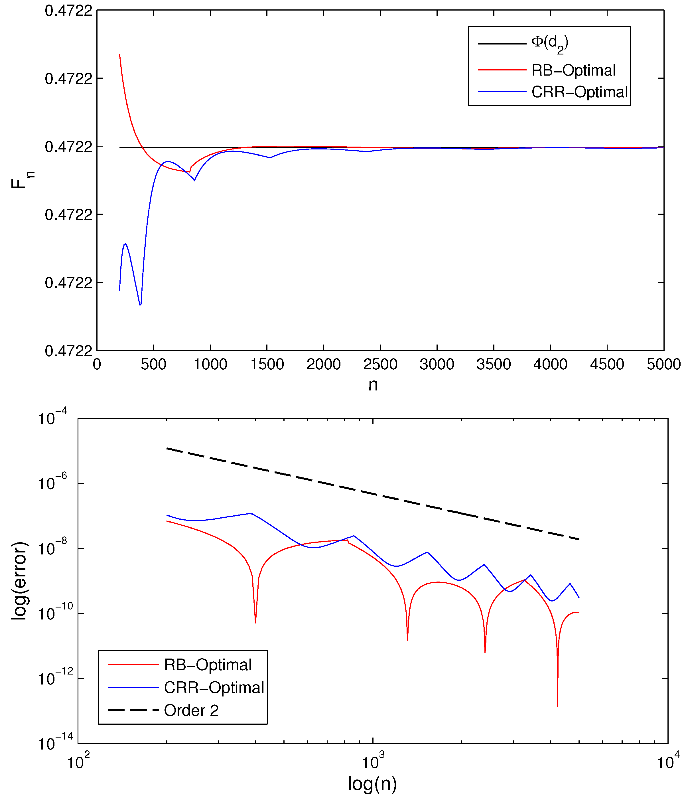
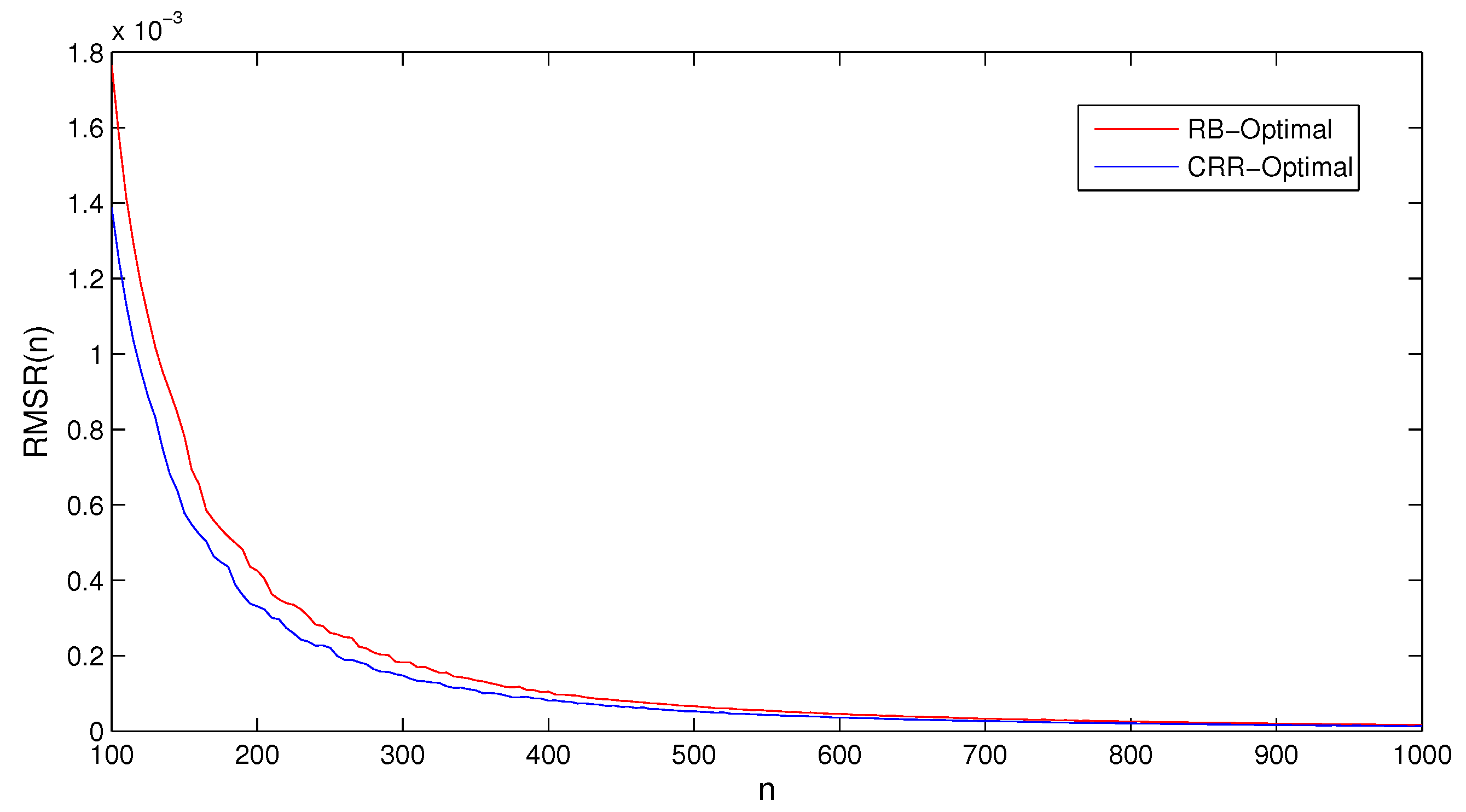
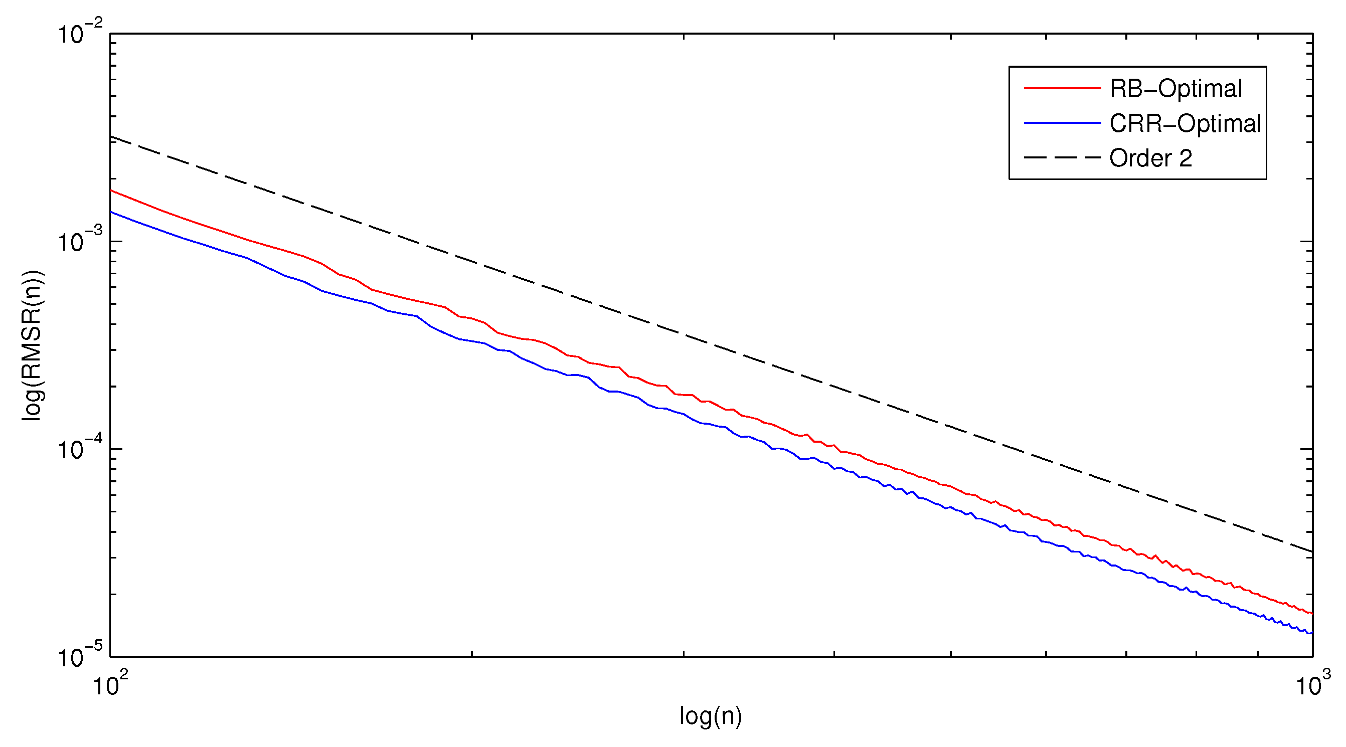
Consider the following log-log plots with the convergence behavior of the 3/2-optimal RB-based and CRR-based trees. By Proposition 1, we should see the slope of $-2$ in the graph. The convergence is not smooth, and the graph is not a straight line; however, the general trend is present.

Figure 1 suggests that the RB-based model gives a slightly better distributional fit. However, to compare the performance of the RB-based and the CRR-based variants for different choices of the coefficient $k_{0,n}$, we consider a whole set of approximation tasks. The performance will be measured in term of both the root mean squared (RMS) error and the root mean squared relative (RMSR) error.

First, we randomly generate a sample of m parameter vectors $\pi =(s_0,x,r,\sigma ,T)$, following the procedure described in [19], but allowing a slightly wider range for the parameters.

• The initial asset price $s_0$ is fixed to 100,
• the value x is uniformly distributed between 50 and 150,
• the riskless interest rate r is uniformly distributed between zero and $0.2$,
• the volatility σ is uniformly distributed between $0.1$ and $0.8$,
• the maturity T is chosen uniformly between zero and one years with probability $0.75$ and between one and five years with probability $0.25$.

Note that $s_0$ remains fixed, and we only vary x as we are only interested in the ratio $\frac{x}{s_0}$. Parameter vectors, for which ${\Phi }^{\pi }\left(d_2\left(x\right)\right)\le {10}^{-6}$, are excluded from the sample to ensure a reliable relative error estimate. For each $n\in \mathbb{N}$ and every parameter vector π, let ${\epsilon }_{abs}^{\pi }\left(n\right)$ and ${\epsilon }_{rel}^{\pi }\left(n\right)$ denote the absolute and relative error, respectively, i.e.,

$${\epsilon }_{abs}^{\pi }\left(n\right)=\left|F_n^{\pi }\left(x\right)-{\Phi }^{\pi }\left(d_2\left(x\right)\right)\right|,{\epsilon }_{rel}^{\pi }\left(n\right)=\frac{{\epsilon }_{abs}^{\pi }\left(n\right)}{{\Phi }^{\pi }\left(d_2\left(x\right)\right)}$$

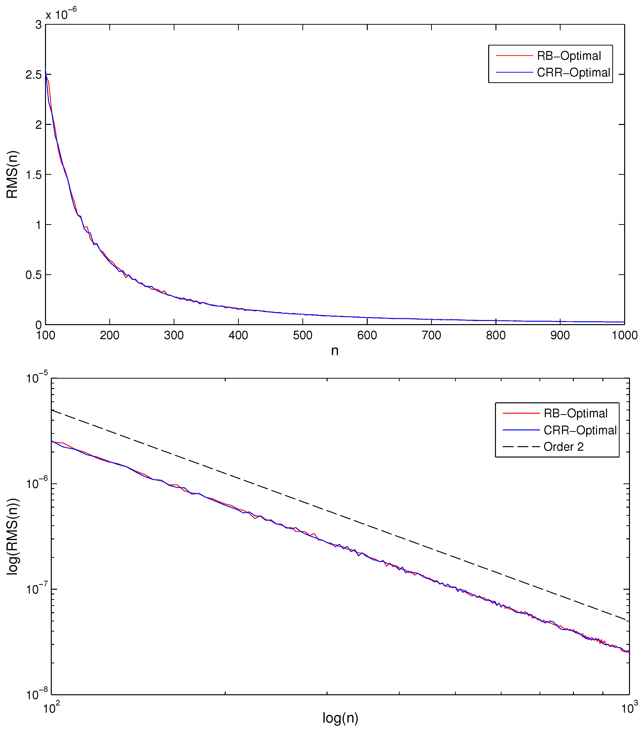
where $F_n^{\pi }$ and ${\Phi }^{\pi }$ refer to the distribution functions of the discrete- and continuous-time models, corresponding to the parameters π. Then, we look at:

$$RMS\left(n\right)=\sqrt{\frac{1}{m}{\displaystyle \sum _{i=1}^m}{\left({\epsilon }_{abs}^{{\pi }_i}\left(n\right)\right)}^2},RMSR\left(n\right)=\sqrt{\frac{1}{m}{\displaystyle \sum _{i=1}^m}{\left({\epsilon }_{rel}^{{\pi }_i}\left(n\right)\right)}^2}$$

Due to Proposition 1, both errors are of order $O\left(\frac{1}{n^2}\right)$. Consider the following convergence behavior of the errors, taken over a sample of $m=1000$ parameter vectors, 995 of which are included. For both errors, a maximum of $n=1000$ time steps is considered.

Note that the absolute error has a very similar convergence pattern for both models (see Figure 2). However, Figure 3 suggests that the CRR-optimal tree delivers better results for the relative error.

4. Expansions for Barrier Option Prices

We now apply the above results to improve the convergence behavior for barrier options.

To examine the performance of our new approach, we will focus on the price of an up-and-in put option with payoff:

$${\left(K-S\left(T\right)\right)}^{+} 1_{\left\{S\left(t\right)\ge B,\text{for some} t\in \left[0,T\right]\right\}}$$

Prices of other barrier options can be obtained in a similar manner or using the in-out parities for single barrier options. We assume $s_0<B$, as otherwise, the barrier option becomes a plain vanilla option. Let $K<B$; then, the price of an up-and-in put is given by (see, e.g., [20]):

$$\begin{array}{c}\hfill V_P^{ui}=K{e}^{-rT}{\left(\frac{B}{s_0}\right)}^{\mu }\Phi \left(d_3\right)-s_0{\left(\frac{B}{s_0}\right)}^{\mu +2}\Phi \left(d_4\right)\end{array}$$

where $\mu =\frac{2r}{{\sigma }^2}-1$ and:

$$d_3=\frac{log\left(\frac{K{s}_0}{B^2}\right)-\left(r-\frac{1}{2}{\sigma }^2\right)T}{\sigma \sqrt{T}},d_4=d_3-\sigma \sqrt{T}$$

Lattice methods for barrier options have a very irregular convergence behavior due to the position of the barrier. This phenomenon, as well as possible solutions have been studied by various authors; see, for example, [5,6,21], etc. A first order asymptotic expansion for binomial trees has been obtained in [22]. An expansion for barrier options with coefficients up to order $O\left(\frac{1}{n^{3/2}}\right)$ has already been provided in [10]. Here, we show how the Edgeworth expansion (Corollary 1) can be used to increase the order of convergence to $O\left(\frac{1}{n^{3/2}}\right)$.

4.1. Binomial Trees for Barrier Options

Consider the model:

$$S_k^{\left(n\right)}=S_{k-1}^{\left(n\right)}{e}^{\sigma \sqrt{\Delta t}{\xi }_k^{\left(n\right)}},k=1\cdots ,n$$

(14)

with the probability of an up-jump given by:

$$p_n=\frac{1}{2}+c_{1,n}\frac{1}{\sqrt{n}}+c_{2,n}\frac{1}{n}+c_{3,n}\frac{1}{{\sqrt{n}}^3}$$

(15)

where:

$$c_{1,n}=\frac{r-\frac{1}{2}{\sigma }^2}{2\sigma }\sqrt{T}$$

and $c_{2,n},c_{3,n}$ are bounded. We set:

$$\begin{array}{cc}\hfill V_n^{ui}& =E_n\left(e^{-rT}\left(K-S_n^{\left(n\right)}\right)1_{\left\{{max}_{1\le k\le n}{S}_k^{\left(n\right)}\ge B,S_n^{\left(n\right)}\le K\right\}}\right)\hfill \end{array}$$

Let:

$$\begin{array}{cc}\hfill a_n^K& =\frac{log\left(\frac{K}{s_0}\right)}{\sigma \sqrt{\Delta t}},a_n^B=\frac{log\left(\frac{B}{s_0}\right)}{\sigma \sqrt{\Delta t}},l_n^B=⌈a_n^B⌉\hfill \end{array}$$

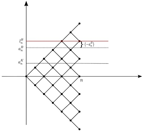
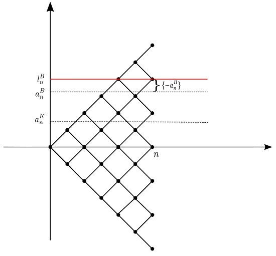
Then, $\left\{-a_n^B\right\}$ is the overshoot of the barrier in the discrete model (Figure 4).

Therefore, we get:

$$\begin{array}{cc}\hfill V_n^{ui}& =\sum _{x\le a_n^K}{E}_n\left(e^{-rT}\left(K-s_0{e}^{\sigma \sqrt{\Delta t}{\sum }_{i=1}^n{\xi }_i^{\left(n\right)}}\right)1_{\left\{{max}_{1\le k\le n}{\sum }_{i=1}^k{\xi }_i^{\left(n\right)}\ge a_n^B,{\sum }_{i=1}^n{\xi }_i^{\left(n\right)}=x\right\}}\right)\hfill \\ & =e^{-rT}K\sum _{x\le a_n^K}P\left(\underset{1\le k\le n}{max}{\displaystyle \sum _{i=1}^k}{\xi }_i^{\left(n\right)}\ge l_n^B,{\displaystyle \sum _{i=1}^n}{\xi }_i^{\left(n\right)}=x\right)\hfill \\ & -s_0\sum _{x\le a_n^K}{e}^{-rT+\sigma \sqrt{\Delta t}·x}P\left(\underset{1\le k\le n}{max}{\displaystyle \sum _{i=1}^k}{\xi }_i^{\left(n\right)}\ge l_n^B,{\displaystyle \sum _{i=1}^n}{\xi }_i^{\left(n\right)}=x\right)\hfill \end{array}$$

(16)

To calculate the probabilities in Equation (16), we need the following lemma that makes use of the reflection principle for a simple random walk. Its proof is similar to that of the continuous-time analogue and can be found in [17].

Lemma 1. 

Let $S_n:=X_1+\cdots +X_n$, where $X_i$ are i.i.d, $X_i=\pm 1$ with probabilities p and q. Then:

$$P\left(\underset{1\le k\le n}{max}{S}_k\ge b,S_n=x\right)=\left\{\begin{array}{cc}{\left(\frac{p}{q}\right)}^{b}P\left(S_n=x-2b\right),\hfill & if x<b\hfill \\ P\left(S_n=x\right),\hfill & if x\ge b\hfill \end{array}\right.$$

(17)

Substituting Lemma 1 into Equation (16), we get:

$$\begin{array}{c}{e}^{-rT}K\sum _{x\le a_n^K}P\left(\underset{1\le k\le n}{max}{\displaystyle \sum _{i=1}^k}{\xi }_i^{\left(n\right)}\ge l_n^B,{\displaystyle \sum _{i=1}^n}{\xi }_i^{\left(n\right)}=x\right)\hfill \\ =e^{-rT}K{\left(\frac{p}{q}\right)}^{l_n^B}\sum _{x\le a_n^K}P\left({\displaystyle \sum _{i=1}^n}{\xi }_i^{\left(n\right)}=x-2l_n^B\right)=e^{-rT}K{\left(\frac{p}{q}\right)}^{l_n^B}P\left({\displaystyle \sum _{i=1}^n}{\xi }_i^{\left(n\right)}\le a_n^K-2l_n^B\right)\hfill \end{array}$$

To get the dynamics of the second term in Equation (16), we need to perform a suitable change of measure. Let:

$${\lambda }_{n,k}=e^{\left(-r\right)\Delta t+\sigma \sqrt{\Delta t}{\xi }_k^{\left(n\right)}},k=1,\cdots ,n$$

and:

$$M_n=E\left({\lambda }_{n,1}\right)$$

(18)

We can now define new transition probabilities for ${\xi }_k^{\left(n\right)}$, $k=1,\cdots ,n$. Let the new probabilities of an up-jump ${\tilde{p}}_n$ and a down-jump ${\tilde{q}}_n$ be:

$$\begin{array}{ccc}\hfill {\tilde{p}}_n& =& \frac{e^{\left(-r\right)\Delta t+\sigma \sqrt{\Delta t}}{p}_n}{M_n}\hfill \end{array}$$

(19)

$$\begin{array}{ccc}\hfill {\tilde{q}}_n& =& \frac{e^{\left(-r\right)\Delta t-\sigma \sqrt{\Delta t}}(1-p_n)}{M_n}\hfill \end{array}$$

(20)

Note that ${\tilde{p}}_n,{\tilde{q}}_n$ are well defined, starting from some $n\in \mathbb{N}$, and ${\tilde{p}}_n+{\tilde{q}}_n=1$. The new probability measure ${\tilde{P}}_n$ is now defined as:

$$\begin{array}{c}{\tilde{P}}_n\left({\omega }_1,\cdots ,{\omega }_n\right)={\tilde{p}}_n^{n_u\left({\omega }_1,\cdots ,{\omega }_n\right)}·{\tilde{q}}_n^{n_d\left({\omega }_1,\cdots ,{\omega }_n\right)}\hfill \\ ={\left(\frac{e^{\left(-r\right)\Delta t+\sigma \sqrt{\Delta t}}{p}_n}{M_n}\right)}^{n_u\left({\omega }_1,\cdots ,{\omega }_n\right)}{\left(\frac{e^{\left(-r\right)\Delta t-\sigma \sqrt{\Delta t}}(1-p_n)}{M_n}\right)}^{n_d\left({\omega }_1,\cdots ,{\omega }_n\right)}\hfill \\ ={\displaystyle \prod _{k=1}^n}\frac{{\lambda }_{n,k}\left({\omega }_k\right)}{M_n}{P}_n\left({\omega }_1,\cdots ,{\omega }_n\right)\hfill \end{array}$$

(21)

where ${\omega }_k\in \left\{-1,1\right\}$, $k=1,\cdots n$ and $n_u\left({\omega }_1,\cdots ,{\omega }_n\right)$ and $n_d\left({\omega }_1,\cdots ,{\omega }_n\right)$ are the numbers of ones and $-1$’s in the sequence $\left({\omega }_1,\cdots ,{\omega }_n\right)$. Therefore, the Radon–Nikodým derivative of ${\tilde{P}}_n$ with respect to $P_n$ is given by:

$${\Lambda }_n={\displaystyle \prod _{k=1}^n}\frac{{\lambda }_{n,k}}{M_n}$$

All conditions for a change of measure are now satisfied, and we arrive at:

$$\begin{array}{c}{s}_0\sum _{x\le a_n^K}{e}^{-rT+\sigma \sqrt{\Delta t}·x}P\left(\underset{1\le k\le n}{max}{\displaystyle \sum _{i=1}^k}{\xi }_i^{\left(n\right)}\ge l_n^B,{\displaystyle \sum _{i=1}^n}{\xi }_i^{\left(n\right)}=x\right)\hfill \\ =s_0{\left(\frac{p}{q}\right)}^{l_n^B}\sum _{x\le a_n^K}{e}^{-rT+\sigma \sqrt{\Delta t}·x}P\left({\displaystyle \sum _{i=1}^n}{\xi }_i^{\left(n\right)}=x-2l_n^B\right)\hfill \\ =s_0{\left(\frac{p}{q}\right)}^{l_n^B}{e}^{2l_n^B\sigma \sqrt{\Delta t}}{M}_n^n\tilde{P}\left({\displaystyle \sum _{i=1}^n}{\xi }_i^{\left(n\right)}\le a_n^K-2l_n^B\right)\hfill \end{array}$$

As a result, we obtain:

$$\begin{array}{cc}\hfill V_n^{ui}& =e^{-rT}K{\left(\frac{p}{q}\right)}^{l_n^B}P\left({\displaystyle \sum _{i=1}^n}{\xi }_i^{\left(n\right)}\le a_n^K-2l_n^B\right)\hfill \\ & -s_0{\left(\frac{p}{q}\right)}^{l_n^B}{e}^{2l_n^B\sigma \sqrt{\Delta t}}{M}_n^n\tilde{P}\left({\displaystyle \sum _{i=1}^n}{\xi }_i^{\left(n\right)}\le a_n^K-2l_n^B\right)\hfill \end{array}$$

(22)

Proposition 2. 

With an appropriate choice of coefficients $c_{2,n}$ and $c_{3,n}$, the binomial model in Equation (14) satisfies:

$$V_n^{ui}=V^{ui}+O\left(\frac{1}{{\sqrt{n}}^3}\right)$$

The proof of the proposition and the possible choice of the coefficients $c_{2,n}$ and $c_{3,n}$ are provided in Appendix C. We call the resulting modified binomial tree the 1-optimal tree.

Remark 6. 

Consider the leading error coefficient in Equation (C9). Note that $g_{1,n}$, $g_{2,n}$ are constant; therefore, the oscillatory convergence behavior is due to the overshoot of the barrier $\left\{-a_n^B\right\}$. The relative position of the strike with respect to the two neighboring nodes at maturity does not enter into the expression. The strike is only present starting from the $O\left(\frac{1}{n}\right)$ coefficient in the term $S_1\left(a_n\right)$ together with the barrier in quadratic form. Therefore, the position of the barrier will have a much stronger effect on the convergence pattern than the position of the strike (see also [10]).

4.2. Numerical Results

We now consider the convergence pattern of a specific barrier option.

Remark 7. 

Note that as in the CRR tree, we have $c_{2,n}=0$; the leading error coefficient in Equation (C9) becomes $\left\{-a_n^B\right\}{g}_{2,n}$, where $0<\left\{-a_n^B\right\}\le 1$. Therefore, the binomial tree will either overestimate or underestimate the BS price for all n, depending on the sign of $g_{2,n}$, as can be seen in Figure 5 and Figure 6.

CRR vs. RB

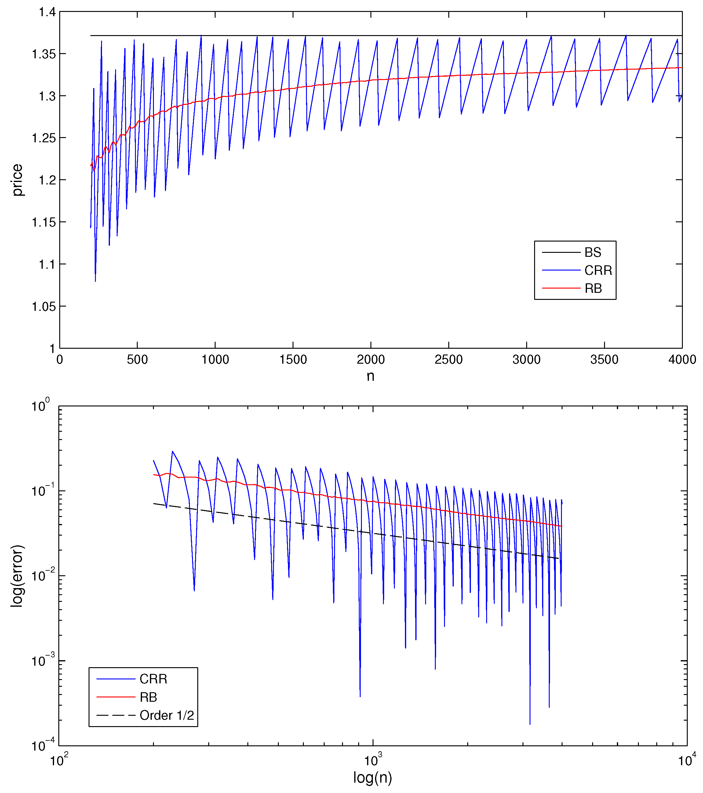
For barrier options, we have a different behavior for the RB and the CRR trees. Expansions for the RB tree cannot be obtained with the method described above, since the reflection principle is directly applicable only to the CRR tree; however, numerical results show that the RB tree has a much smoother convergence compared to the CRR tree. This can be explained by the fact that, as the CRR tree is symmetric around zero in the log-scale, the overshoot of the barrier $\left\{-a_n^B\right\}$ is the same for each time step. Therefore, with an increase of n, a whole row of nodes becomes out-of-the-money. The RB tree, on the other hand, is tilted; therefore, this effect is not that pronounced.

See Figure 5 for the numerical illustration of this behaviour.

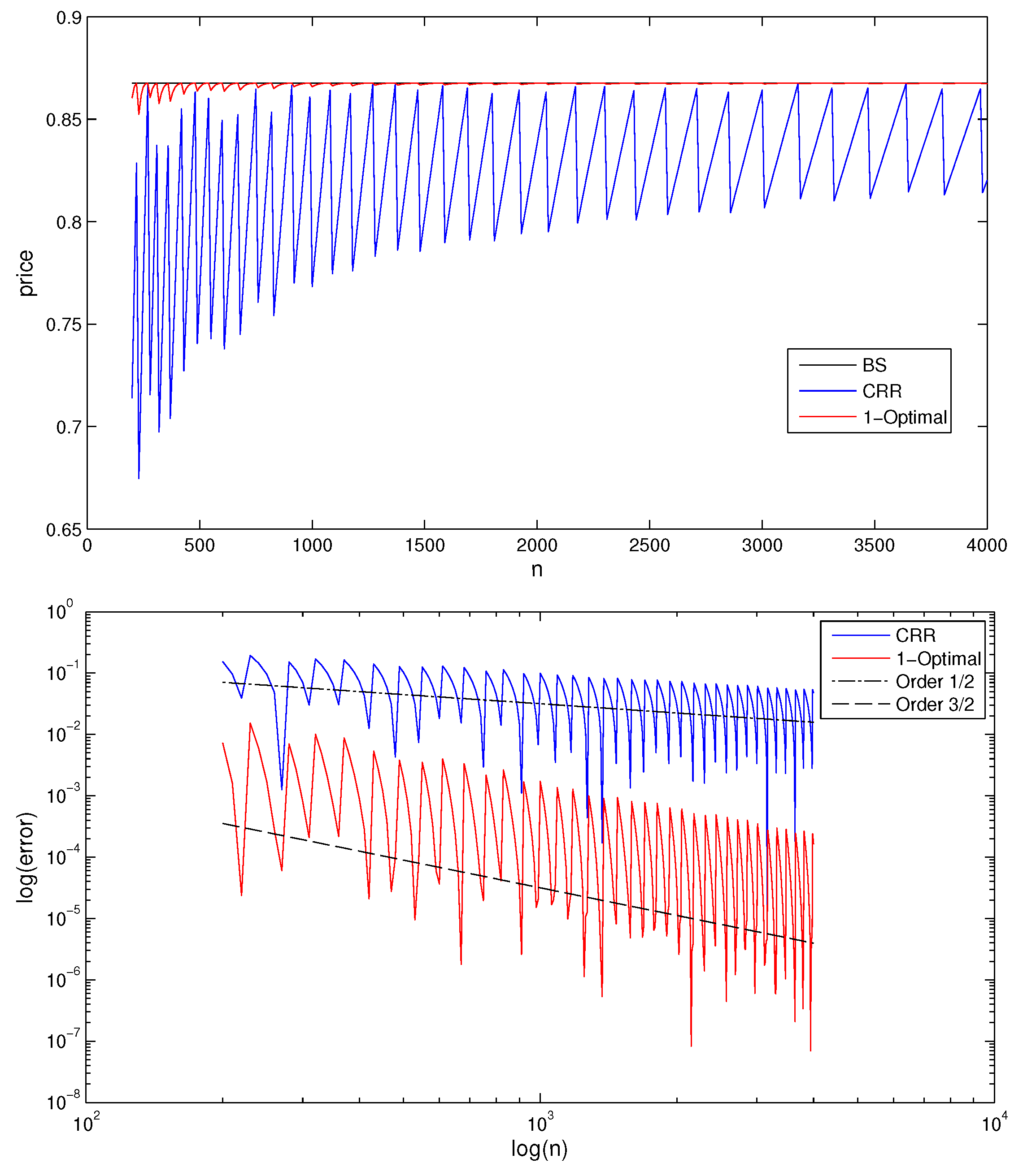
Figure 6 illustrates the superior behaviour of the 1-optimal tree compared to the CRR-tree.

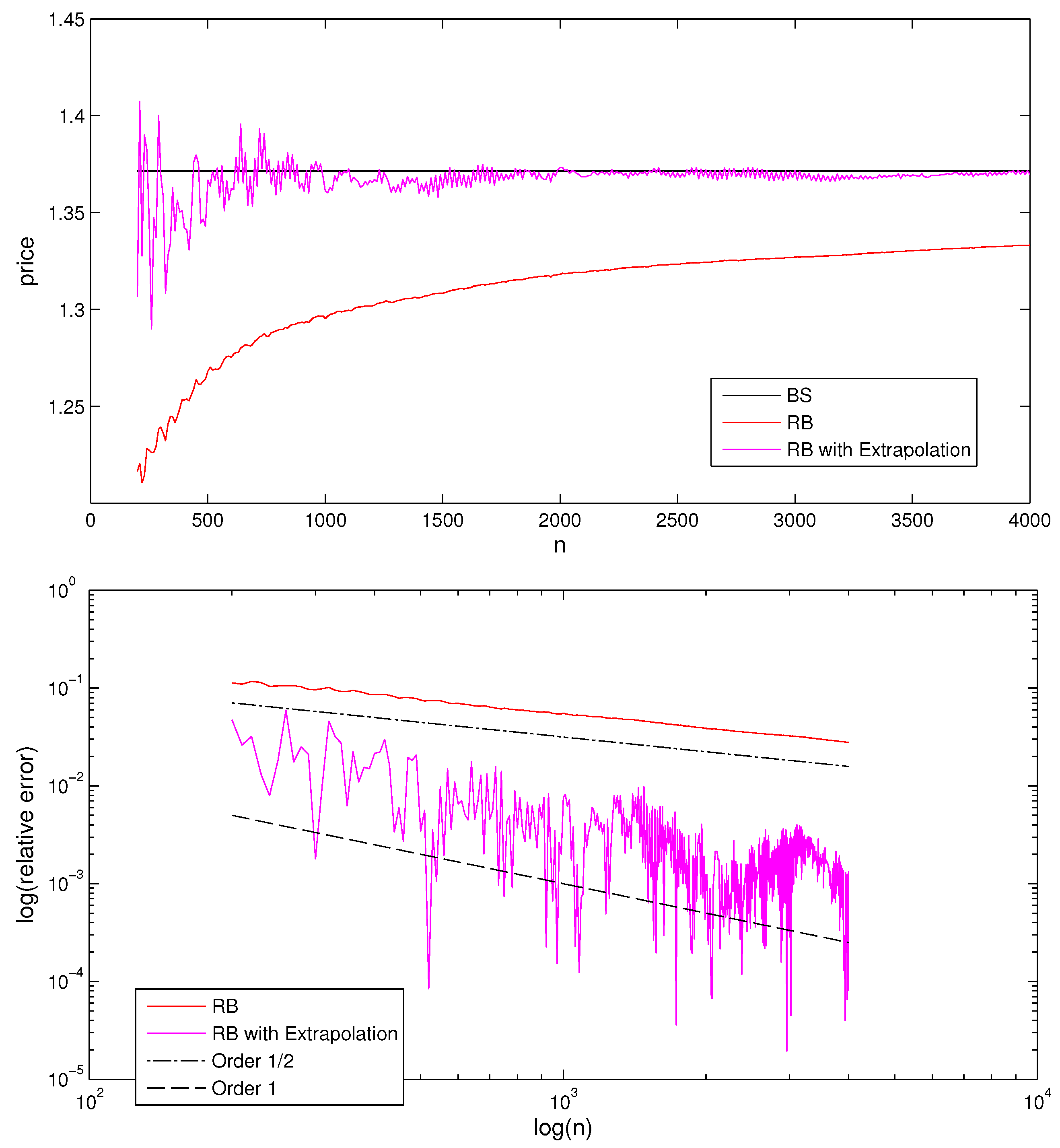
Due to the smooth convergence pattern, we can apply extrapolation to the RB tree to increase the order of convergence(see Figure 7).

Although the RB tree with extrapolation outperforms the CRR tree, the 1-optimal tree outperforms the two others by far. This observation is summarized in

Table 1. Convergence behaviour of CRR, RB with extrapolation and the 1-optimal tree.

Parameters	n	CRR Tree	RB Extrapolation	1-Optimal	BS Value
$T=1$	100	1.0370950	1.2728844	1.3071811	1.3714613
$s_0=100$	200	1.1428755	1.3064705	1.3528020
$K=110$, $B=120$	500	1.2210427	1.3667218	1.3668495
$\sigma =0.25$	1000	1.2248525	1.3608690	1.3671287
$r=0.1$	2000	1.3285299	1.3731534	1.3713814
	4000	1.3018025	1.3696310	1.3710375

below.

5. Conclusions

We have considered applications of the Edgeworth expansions to one-dimensional tree models in the Black–Scholes setting. We have seen how expansions can be obtained for barrier options and how these results can be used to improve convergence behavior. For applications to digital and European options, as well as multidimensional trees, see [17].

Once again, we consider the binomial method as a purely numerical approach and do not restrict ourselves to the equivalent martingale measure in the binomial setting. This gives us more freedom in the construction of the advanced trees, as it allows one to choose the probabilities, as well as the drift of the tree. Nevertheless, the expansions obtained in the proofs of the propositions above hold for a very general setting and can also be applied to trees under the risk-neutral measure.

References

- J.C. Cox, S.A. Ross, and M. Rubinstein. “Option Pricing: A Simplified Approach.” J. Financ. Econ. 7 (1979): 229–263. [Google Scholar] [CrossRef]
- R.J. Rendleman, and B.J. Bartter. “Two-State Option Pricing.” J. Financ. 34 (1979): 1093–1110. [Google Scholar] [CrossRef]
- P. Billingsley. Convergence of Probability Measures. New York, NY, USA: J. Wiley & Sons, 1968. [Google Scholar]
- R. Korn, and E. Korn. Option Pricing and Portfolio Optimization. Providence, RI, USA: AMS, 2001. [Google Scholar]
- P.P. Boyle, and S.H. Lau. “Bumping up against the Barrier with the Binomial Method.” J. Deriv. 1 (1994): 6–14. [Google Scholar] [CrossRef]
- P. Ritchken. “On pricing barrier options.” J. Deriv. 3 (1995): 19–28. [Google Scholar] [CrossRef]
- D.P.J. Leisen, and M. Reimer. “Binomial Models for Option Valuation—Examining and Improving Convergence.” Appl. Math. Financ. 3 (1996): 319–346. [Google Scholar] [CrossRef]
- Y.S. Tian. “A Flexible Binomial Option Pricing Model.” J. Future Mark. 19 (1999): 817–843. [Google Scholar] [CrossRef]
- F. Diener, and M. Diener. “Asymptotics of the price oscillations of the European call option in a tree model.” Math. Financ. 14 (2004): 271–293. [Google Scholar] [CrossRef]
- J. Lin, and K. Palmer. “Convergence of barrier option prices in the binomial model.” Math. Financ. 23 (2013): 2318–2338. [Google Scholar]
- L.-B. Chang, and K. Palmer. “Smooth Convergence in the Binomial Model.” Financ. Stoch. 11 (2007): 91–105. [Google Scholar] [CrossRef]
- M. Joshi. “Achieving higher order convergence for the prices of European options in binomial trees.” Math. Financ. 20 (2010): 89–103. [Google Scholar] [CrossRef]
- R. Korn, and S. Müller. “The optimal-drift model: An accelerated binomial scheme.” Financ. Stoch. 17 (2013): 135–160. [Google Scholar] [CrossRef]
- M. Rubinstein. “Edgeworth binomial trees.” J. Deriv. 5 (1998): 20–27. [Google Scholar] [CrossRef]
- S. Müller. “The Binomial Approach to Option Valuation.” Ph.D. Thesis, University of Kaiserslautern, Kaiserslautern, Germany, 2009. [Google Scholar]
- J.V. Uspensky. Introduction to Mathematical Probability. New York, NY, USA: McGraw-Hill, 1937. [Google Scholar]
- A. Bock. “Edgeworth Expansions for Binomial Trees.” Ph.D. Thesis, University of Kaiserslautern, Kaiserslautern, Germany, 2014. [Google Scholar]
- G. Leduc. “Arbitrarily Fast CRR Schemes; Working Paper.” Available online: https://mpra.ub.uni-muenchen.de/42094/ (accessed on 21 October 2012).
- M. Broadie, and J. Detemple. “American option valuation: New bounds, approximations and a comparison for existing methods.” Rev. Financ. Stud. 9 (1996): 1221–1250. [Google Scholar] [CrossRef]
- E.G. Haug. The Complete Guide to Option Pricing Formulas. New York, NY, USA: McGraw-Hill, 2006. [Google Scholar]
- E. Derman, I. Kani, D. Ergener, and I. Bardhan. “Enhanced numerical methods for options with barriers.” Financ. Anal. J. 51 (1995): 8–17. [Google Scholar] [CrossRef]
- E. Gobet. Analysis of the Zigzag Convergence for Barrier Options With Binomial Trees. Working paper 536; Paris, France: Université Paris 6 et Paris7, 1999. [Google Scholar]
- R.N. Bhattacharya, and R.R. Rao. Normal Approximation and Asymptotic Expansions. Berlin, Germany; New York, NY, USA: de Gruyter, 1976. [Google Scholar]
- A. Bock. “Edgeworth Expansions for lattice triangular arrays.” In Report in Wirtschaftsmathematik (WIMA Report). Kaiserslautern, Germany: University of Kaiserslautern, 2014, Volume 149. [Google Scholar]
- I.A. Korchinsky, and A.M. Kulik. “Local limit theorems for triangular array of random variables.” Theory Stoch. Process. 13 (2007): 48–54. [Google Scholar]
Figure 1.
Distributional fit with , , , , .
Figure 2.
and error.
Figure 3.
Figure 4.
Dynamics of .
Figure 5.
CRR vs. RB: up-and-in barrier put, , , , , , .
Figure 6.
CRR vs. 1-opt.: Up-and-in barrier put, , , , , , .
Figure 7.
RB with extrapolation: up-and-in barrier put with , , , , , .