Ruin Probabilities with Dependence on the Number of Claims within a Fixed Time Window

Abstract

We analyse the ruin probabilities for a renewal insurance risk process with inter-arrival times depending on the claims that arrive within a fixed (past) time window. This dependence could be explained through a regenerative structure. The main inspiration of the model comes from the bonus-malus (BM) feature of pricing car insurance. We discuss first the asymptotic results of ruin probabilities for different regimes of claim distributions. For numerical results, we recognise an embedded Markov additive process, and via an appropriate change of measure, ruin probabilities could be computed to a closed-form formulae. Additionally, we employ the importance sampling simulations to derive ruin probabilities, which further permit an in-depth analysis of a few concrete cases.

1. Introduction

With the ever growing popularity of bonus-malus systems in the car insurance industry, one interesting question to study is whether it really reduces the associated risk and by how much. A common measure to assess risks that an insurer is exposed to is the so-called ruin probability. Motivated by such questions, we derive ruin probabilities in models with a dependence structure that captures the key feature of a simple bonus system, namely that there is a premium discount when no claims are observed in the previous year. Inspired by this feature, we found a regenerative structure within inter-claim times that could describe the properties of an analogous bonus system, also referred to as a no claims discount (NCD) system.

In the classical collective risk insurance model, the independence among inter-claim times is one of the crucial assumptions. However, in reality, one could easily find violations of such an assumption. For instance, in car insurance, if there has been a long waiting time before a claim, the next inter-arrival time can be long, as well, because the policyholders are potentially “good drivers”; or it could be the other way around, where some policyholders only start to use their cars a long time after purchasing them, then claims would suddenly arrive more frequently after a long silence. Hence, a shorter interval before the next claim can be expected. Therefore, a natural way to relax this assumption is to introduce a dependence structure in-between inter-arrival times, and that is the main purpose of this paper.

For the simplest case, comparing the current time since the last claim with a fixed threshold ξ (either exceeded or not exceeded) determines the distribution for the time until the next claim. A risk-lover insurer can set a larger mean for the following claim interval, whereas a risk-averse one will possibly choose a lower mean. We will use $\tilde{\tau }$ to denote the subsequent random inter-arrival time when the current one is larger than ξ. The graph on the left in Figure 1 shows a sample path of this underlying risk surplus process.

Figure 1 illustrates how a change of inter-arrival time distribution could equivalently be represented by a modification in the premium rate. Let us denote an arbitrary inter-claim time by τ. The left graph shows a risk surplus process with inter-arrival times switching between two different random variables according to the dependence structure addressed earlier, whereas the graph on the right presents a two-level premium varying risk surplus process where the premium rate decreases after a relatively long wait, which exceeds a fixed number ξ, i.e., a bonus for no claims. After that, since the second waiting interval is less than ξ, the premium rate returns to its original value, and so on and so forth.

Clearly, the inter-arrival times switching between two different random variables can be reflected by adjustment on premium rates, as long as the increment of the surplus process $U(t)$ in this time interval is kept the same, where $U(t)$ as a function of time describes the reserve level overtime as defined by Equation (1). That is to say, whenever a large inter-arrival time that is above ξ is witnessed, the next inter-claim time will switch to a random variable $\tilde{\tau }$ with a different distribution. Notice that the two models presented in Figure 1 are equivalent only when working with ruin probabilities under an infinite-time horizon, but not for a finite-time case.

These graphs also suggest that our proposed model could also, to some extent, mimic the nature of a no claim discount (NCD) system. This term refers to a simplified bonus-malus (BM) system, a bonus system, with only premium discounts when there are no claims witnessed in a fixed time window. We can thus naturally draw the analogy between a bonus-only system and the risk model with these two-level varying premiums. Although we cannot equate them because the NCD systems are for individual risks, the feature of varying premiums could be generalised to the collective level. For instance, in the case where no claims are reported to the insurer in a fixed time period, the premium rate could see a slight decrease because of all individuals’ premium discounts. Looking back at Figure 1, $\tilde{\tau }$ could be assumed to have a smaller mean than τ for the interpretation resulting from the effect of a drop in the premium rate. The opposite case implies a malus-only system, which is not often seen in practice. However, as mentioned before, a conservative insurer might choose this option. Additionally, for computational reasons, we make the assumption that the inter-exchange of the randomness of inter-arrival times only happens after a jump rather than precisely at the end of the fixed window.

In risk theory, one of the extensions from a classical collective risk model involves the relaxation of the assumption of independence. Hence, dependence models have been introduced under a risk theory framework in various kinds of ways. For a dependence within claims, Albrecher et al. [1] calculated ruin probabilities by using Archimedean survival copulas. Through a copula method, Valdez and Mo [2] also worked with risk models with dependence among claim occurrences focusing more on the simulation side. The dependence between claim sizes and inter-arrival times was also analysed. Albrecher and Boxma [3] first considered the case when the inter-claim time depends on the previous claim size with a random threshold. Due to the complexity of inverting Laplace transform, they could only obtain the results in terms of Laplace transforms. Kwan and Yang [4] then studied such a dependence structure with a deterministic threshold, and they were able to express ruin probability explicitly by solving a system of ordinary delay differential equations. Furthermore, Constantinescu et al. [5] also considered risk processes with various forms of dependence between inter-arrival times and claim sizes. This work though aims at adjusting premiums dynamically in order to meet the solvency requirement on the ruin probability for a fixed initial reserve using the idea developed by Dubey [6], rather than calculating the probability of ruin.

On the other hand, we have included some references here to remind the readers of the concept of bonus-malus systems, as well as research that has attempted studying the risks associated with this kind of systems. Most of the research on bonus-malus systems mainly relied on the construction of a discrete time Markov chain in order to compute different levels of prices; see, e.g., Lemaire [7]. Due to the possibility of slow convergence to stationarity, Asmussen [8] added an age-correction and implemented numerical analyses for various bonus-malus systems in different countries. Instead of considering premium levels depending only on claims in the previous period, it is alternatively suggested to take into account the entire history where a Bayesian view could be adopted as in Asmussen [8]. A recent work by Ni et al. [9] also applied the Bayesian approach to reflect this idea and obtained premiums in a closed form when claim severities are assumed to be Weibull distributed.

There have been a few papers investigating ruin probabilities for a bonus-malus system recently. Working with real data, Afonso et al. [10] calculated ruin probabilities under a realistic bonus-malus framework and found an increase in ruin probability for a closed portfolio due to reduced income. The idea in their article, which was earlier developed in Afonso et al. [11] is that they first analyse ruin probabilities for a single year conditioning on the reserve levels at the beginning and the end of the year. Since the premium rate is kept constant within a year, a classical technique could be borrowed. Then, they use approximations and estimate ruin probabilities numerically. On the other hand, the incorporation of the feature of a bonus-malus system into a risk model is similar to a variation in the premium rates after a claim arrival. For such a dependence, by employing a Bayesian estimator in a risk model and using a comparison method with the classical case, Dubey [6] and Li et al. [12] could interpret ruin probabilities in terms of a classic one. In this paper, we follow a similar idea. However, our work here is to model the dependence between premium rates and the claim arrivals within a fixed time window. In our opinion, it mimics better the key feature of a bonus system. The consequence of this approach is that it implies modelling the dependence between two consecutive inter-claim times based on a fixed threshold. This serves as the main goal of this work. Furthermore, the allowance of such dependence obviously violates the renewal property as in the classical model. Nevertheless, a regenerative structure can be identified so that analyses are possible. For the literature on regenerative processes, we refer to Palmowski and Zwart [13,14].

Aiming at studying the ruin probability for a risk model with dependent inter-claim times, we try to investigate this model under a regenerative framework using various methods. We start by looking at some asymptotic results via adopting theories developed for general regenerative processes in Palmowski and Zwart [13,14]. For the Cramér case, it still shows exponential tails for the probability of ruin. All asymptotic results are shown for a general situation where the distribution for each random variable is not specified. Then, by constructing an appropriate Markov additive process and using the importance sampling method, we can run simulations to get numerical results for the case where inter-claim times and claims are exponentially distributed. In the end, we employ the crude Monte Carlo simulations to compare the underlying ruin probability with a classic one as a case analysis. In addition, we look at the influence of claim distributions on the ruin probabilities, where we found that there is no significant differences in ruin probabilities when altering between exponential and Pareto claims. In general, results suggest that the use of bonus systems may not act in favour of the reduction on ruin probabilities. That is probably because premium discounts generally decrease the risk reserves.

2. The Model

Let us start by describing the model that we will work with in this paper. We denote by $U(t)$ the amount of surplus of an insurance portfolio at time t:

$$U(t)=x+ct-\sum _{k=1}^{N(t)}{Y}_k$$

(1)

In the above classical model Equation (1), c represents the constant rate of premium inflow, $N(t)$ is an arrival process that counts the number of claims incurred during the time interval $(0,t]$ and ${(Y_k)}_{k\ge 0}$ is a sequence of independent and identically distributed (i.i.d.) claim sizes with distribution function $F_Y$ and density $f_Y$ (also independent of the claim arrival process $N(t)$). We assume that $U(t)\to +\infty$ almost surely as $t\to +\infty$. One of the crucial quantities to investigate in this context is the probability that the surplus in the portfolio will not be sufficient to cover the claims for the first time, which is called the probability of ruin:

$$\psi (x)=\mathbb{P}(T(x)<\infty \mid U(0)=x)$$

Here, $U(0)=x\ge 0$ is the initial reserve in the portfolio and

$$T(x)=inf\{t\ge 0:U(t)<0\mid U(0)=x\}$$

is the time of ruin for an initial surplus x. We specify the counting process $N(t)$, which in the classical models is a Poisson process. Let ${({\tau }_k)}_{k\ge 0}$ be the sequence of inter-claim times. In this paper, we analyse the model when the distribution $F_{{\tau }_k}$ of ${\tau }_k$ depends on the number of claims that appeared within a fixed past time window ξ as follows,

$$\mathbb{P}\left({\tau }_k\le x|N\left(\sum _{i=1}^k{\tau }_{i-1}\right)-N\left(\sum _{i=1}^k{\tau }_{i-1}-\xi \right)=n\right)=F_{{\tau }_k}\left(x,n\right).$$

It is true that when such a dependence structure is introduced, a direct use of renewal theory is no longer applicable. However, even though it is not renewal at each jump epoch, the process in fact renews after several jumps, and we call this a "regeneration". Thus, we define the regenerative epochs for our model in the following way.

Definition 1. 

Let

$$L_{k+1}=min\left\{l\in \mathbb{N}:l>L_k\mathrm{and}N\left(\sum _{i=1}^l{\tau }_{i-1}\right)-N\left(\sum _{i=1}^l{\tau }_{i-1}-\xi \right)=0\right\}.$$

Then the regeneration epochs $T_{k+1},k=0,1,\dots$ are defined as:

$$T_{k+1}=\sum _{i=1}^{L_{k+1}}{\tau }_{i-1}$$

for $k\ge 0$, with $L_0=0$ and $T_0=0$.

Roughly speaking, at these epochs $T_k$ (the arrival times with a zero number of arrivals within the last time window lagged by ξ) the risk process $U(t)$ loses its ‘memory’, and starting at these epochs, the stochastic evolution remains the same. A formal definition of a regenerative process can be found in Appendix A1 in Asmussen and Albrecher [15]. It easy to observe that the risk process $U(t)$ is indeed regenerative with regeneration epochs $T_k$, $k\in \mathbb{N}$. In this case, $\mathbb{P}({\tau }_l\le x|L_k=l)=F_{{\tau }_l}(x,0)$, for $k\in \mathbb{N}$ and $l\ge k$. Notice that we define the regenerative epochs in such a way that the concern only lies in whether there are claims or not in the past fixed window ξ rather than how many of them there are.

Furthermore, let us consider the claim surplus process denoted by:

$$S(t)=\sum _{k=1}^{N(t)}{Y}_i-c·t$$

and let:

$$M=\underset{t\ge 0}{sup}S(t),M_{n+1}=\underset{T_n\le t<T_{n+1}}{sup}S(t)-S(T_n),\text{for}n\ge 0$$

and:

$$X_{n+1}=S(T_{n+1})-S(T_n)$$

(2)

Then, due to the regenerative structure of the claim surplus process $S(t)$, the discrete-time process $S_n=S(T_n)={\sum }_{i=1}^n{X}_i$ ($n\ge 0$) is a random walk. The crucial observation used in this paper is:

$$\psi (x)=\mathbb{P}(M>x)=\mathbb{P}(\underset{n}{max}(M_n+S_{n-1})>x)$$

(3)

The simplest case that we focus on has inter-claim times following two random variables τ and $\tilde{\tau }$. We choose τ when in a past time-window of length ξ, there is at least one claim; otherwise, we choose $\tilde{\tau }$ as the inter-arrival time. Hence, for $k\in \mathbb{N}$,

$$F_{{\tau }_k}(x,n)=\left\{\begin{array}{l}\mathbb{P}(\tau \le x),\mathrm{for}n\ge 1;\\ \mathbb{P}(\tilde{\tau }\le x),\mathrm{otherwise}\end{array}\right.$$

It is a natural choice since usually in the insurance industry, a long “silence” translates into a different behaviour of the arrival process just right after it. To rephrase it, our current model incorporates a dependence structure between each pair of consecutive inter-arrival times. Whenever an inter-arrival time exceeds ξ, the next one would have the same distribution as $\tilde{\tau }$. Otherwise, it conforms to τ.

More interestingly, as mentioned earlier, one motivation of such a model set-up is the analogy, although not the same, with a basic bonus system, i.e., a system where policyholders enjoy discounts when they do not file claims for a certain period (but with no penalties). Such an analogy is possible given that the premium discounts for individuals in an NCD system could be equivalently reflected by a drop in the premium rates at the collective level. Without loss of generality, Figure 1 plots an example of such risk processes and demonstrates how our model reflects the feature of a bonus system. A sample path of the claim surplus process we will be working with is given in Figure 2 (where we assume starting from $\tilde{\tau }$).

Recall from Equation (2) that $X_1$ is the end value at the first regenerative epoch. Then, it is not difficult to observe that it has the same law as:

$$X_1\stackrel{d}{=}(Y_0-\tilde{\tau })+{\mathbf{I}}_{\{\tilde{\tau }\le \xi \}}\left(\sum _{k=1}^{N-1}(Y_k-{\tau }_k^{\le \xi })+\left(Y_N-{\tau }_N^{>\xi }\right)\right)$$

(4)

where N is a geometrical random variable with parameter $p=\mathbb{P}(\tau >\xi )$. Here, $\mathbb{P}(N=k)={(1-p)}^{k-1}p$, $k=1,2\dots$ and ${\tau }_k^{\le \xi }\stackrel{d}{=}{\tau }_k|{\tau }_k\le \xi$, ${\tau }_k^{>\xi }\stackrel{d}{=}{\tau }_k|{\tau }_k>\xi$. For simplicity, we assume $c=1$ here and throughout the paper.

The paper is organized as follows. Section 3 presents asymptotic results about ruin probabilities under three different regimes for claim distributions, using asymptotics derived for general regenerative processes as in [13,14]. Section 4 demonstrates some numerical results via simulations and discusses a case analysis, including a comparison with ruin in a classical risk model. The simulations used in this section are based on the embedded Markov additive process within our model and rely on the importance sampling method via a change of measure. A few conclusions will be drawn in Section 5.

3. Asymptotic Results

In this section, we look at three different situations for claim distributions and analyse the asymptotic ruin probability associated with each of them. Inter-arrival times considered in this section are general random variables if not mentioned otherwise.

3.1. The Heavy-Tailed Case

Let us first discuss the heavy-tailed case. We start with the assumption that the distribution $F_M$ of the generic $M_1$ belongs to the class $\mathcal{S}$ of subexponential distribution functions, where a distribution function $G\in \mathcal{S}$ on ${\mathbb{R}}_{+}$ if and only if $\overline{G}(x)>0$, for all x, and:

$$\underset{x\to \infty }{lim}\overline{G^{*2}}(x)/\overline{G}(x)=2$$

(5)

(where $G^{*2}$ is the convolution of G with itself). Here, $\overline{G}$ denotes the tail distribution given by $\overline{G}(x)=1-G(x)$. More generally, a distribution function G on $\mathbb{R}$ is subexponential if and only if $G^{+}$ is subexponential, where $G^{+}=G{\mathbf{I}}_{{\mathbb{R}}_{+}}$ and ${\mathbf{I}}_A$ is the indicator function of a set A. We further assume throughout that $F_M\in {\mathcal{S}}^{*}$ are strong subexponential distributions. According to Definition 3.22 in [16], a distribution function G on $\mathbb{R}$ belongs to the class ${\mathcal{S}}^{*}$, i.e., G is strong subexponential, if and only if $\overline{G}(x)>0$, for all x, and:

$${\int }_0^x\overline{G}(x-y)\overline{G}(y)dy\sim 2m_G\overline{G}(x),\text{as}x\to \infty$$

(6)

where:

$$m_G={\int }_0^{\infty }\overline{G}(x)dx$$

is the mean of G. It is again known that the property $G\in {\mathcal{S}}^{*}$ depends only on the tail of G. Further, if $G\in {\mathcal{S}}^{*}$ then $G\in \mathcal{S}$ and also $\overline{G^s}\in {\mathcal{S}}^{*}$ where:

$$\overline{G^s}(x)=min\left(1,{\int }_x^{\infty }\overline{G}(t)dt\right)$$

is the integrated, or second-tail, distribution function determined by G. See [16] for details.

Theorem 2. 

If $\mathbb{E}\left[M_1\right]<\infty$ and $F_M\in {\mathcal{S}}^{*}$, then:

$$\psi (x)\sim \frac{1}{\mu }{\int }_x^{\infty }{\overline{F}}_M(u)\mathrm{d}u$$

(7)

as $x\to \infty$, with $\mu =-\mathbb{E}\left[X_1\right]$.

Proof. 

This proof is similar to Theorem 1 in [13]. ☐

Note that:

$$\mathbb{P}(X_1>x)\le \mathbb{P}(M_1>x)\le \mathbb{P}(X_1+T_1>x)$$

Assume now that τ and $\tilde{\tau }$ are light-tailed, that is there exists $\theta >0$, such that $\mathbb{E}\left[{\mathrm{e}}^{\theta \tau }\right]<\infty$ and $\mathbb{E}\left[{\mathrm{e}}^{\theta \tilde{\tau }}\right]<\infty$ and that:

$$F_M\in {\mathcal{S}}^{*}$$

(8)

Then, from Foss et al. [16], we have that:

$$\mathbb{P}(M_1>x)\sim \mathbb{P}(X_1>x)$$

(9)

and by Equation (4) and Corollary 3.40 in [16], we have that:

$$\begin{array}{ccc}\hfill {\overline{F}}_M(x)\sim \mathbb{P}(X_1>x)& \sim & \left(\mathbb{P}(\tilde{\tau }>\xi )+\mathbb{E}\left[N+1\right]\mathbb{P}(\tilde{\tau }\le \xi )\right)\mathbb{P}(Y>x)\hfill \\ & =& \left(1-\mathbb{P}(\tilde{\tau }\le \xi )+\frac{\mathbb{P}(\tilde{\tau }\le \xi )(2-\mathbb{P}(\tau \le \xi ))}{1-\mathbb{P}(\tau \le \xi )}\right){\overline{F}}_Y(x)\hfill \end{array}$$

(10)

where Y is a generic claim size. Moreover,

$$\begin{array}{ccc}\hfill \mu & =& (\mathbb{E}\left[\tilde{\tau }\right]-\mathbb{E}\left[Y\right])+\left[\mathbb{E}\left[N-1\right]\left(\mathbb{E}\left[{\tau }^{\le \xi }\right]-\mathbb{E}\left[Y\right]\right)+(\mathbb{E}\left[{\tau }^{>\xi }\right]-\mathbb{E}\left[Y\right])\right]\mathbb{P}(\tilde{\tau }\le \xi )\hfill \\ & =& \mathbb{E}\left[\tilde{\tau }\right]-\mathbb{E}\left[Y\right]-\mathbb{P}(\tilde{\tau }\le \xi )\mathbb{E}\left[N\right]\mathbb{E}\left[Y\right]+\mathbb{E}\left[N-1\right]\mathbb{E}\left[\tau |\tau \le \xi \right]\mathbb{P}(\tilde{\tau }\le \xi )+\mathbb{E}\left[\tau |\tau >\xi \right]\mathbb{P}(\tilde{\tau }\le \xi )\hfill \end{array}$$

with:

$$\mathbb{E}\left[N\right]=\frac{1}{1-\mathbb{P}(\tau \le \xi )}=\frac{1}{\mathbb{P}(\tau >\xi )}$$

Remark 1. 

Reducing to the Cramér–Lundberg model

By removal of the dependence assumption in our setting, our model will reduce to the classical model. The independent case is referring to the situation when $\mathbb{P}(\tau \le \xi )=\mathbb{P}(\tilde{\tau }\le \xi )$. Substituting this into Equation (10) yields,

$${\overline{F}}_M(x)\sim \frac{1}{1-\mathbb{P}(\tau \le \xi )}{\overline{F}}_Y(x)=\mathbb{E}\left[N\right]{\overline{F}}_Y(x)$$

In addition, it simplifies μ to:

$$\mu =-\mathbb{E}\left[X_1\right]=\mathbb{E}\left[N\right](\mathbb{E}\left[\tau \right]-\mathbb{E}\left[Y\right])$$

According to Equation (7),

$$\psi (x)\sim \frac{\mathbb{E}\left[N\right]}{\mu }{\int }_x^{\infty }{\overline{F}}_Y(u)\mathrm{d}u=\frac{1}{\mathbb{E}\left[\tau \right]-\mathbb{E}\left[Y\right]}{\int }_x^{\infty }{\overline{F}}_Y(u)\mathrm{d}u$$

If we assume $\mathbb{E}\left[Y\right]={\mu }_Y$, $\mathbb{E}\left[\tau \right]=\mathbb{E}\left[\tilde{\tau }\right]=\frac{1}{\lambda }$ and the safety loading to be ρ i.e., $1+\rho =1/\lambda {\mu }_Y$, and knowing that $\mathbb{E}\left[N\right]=1/p$, the above identity could be reduced to:

$$\psi (x)\sim \frac{1}{\frac{1}{\lambda }-{\mu }_Y}{\int }_x^{\infty }{\overline{F}}_Y(u)\mathrm{d}u=\frac{1}{\rho {\mu }_Y}{\int }_x^{\infty }{\overline{F}}_Y(u)\mathrm{d}u$$

(11)

which coincides with the approximated ruin probability for the classic risk model with subexponential claims, as shown by Theorem 1.36 in [17]. ☐

3.2. The Intermediate Case

We now consider the case where $X_1$ satisfies:

$$\mathbb{P}(X_1>x+y)\sim {\mathrm{e}}^{-\alpha y}\mathbb{P}(X_1>x)$$

(12)

for every fixed y, as $x\to \infty$, and:

$$\mathbb{P}(X_1+X_2>x)\sim 2\mathbb{E}\left[{\mathrm{e}}^{\alpha X_1}\right]\mathbb{P}(X_1>x)$$

(13)

This is equivalent to the condition that $X_1^{+}\in \mathcal{S}(\alpha )$. The case $\alpha =0$ is treated in Section 3.1, so we assume $\alpha >0$. Another assumption we make is that:

$$\mathbb{E}\left[{\mathrm{e}}^{\alpha X_1}\right]<1$$

(14)

which implies that Cramér’s condition is not satisfied. Finally, we specify the tail behaviour of $M_1$. The case where $M_1$ has a heavier tail than $X_1$ is already covered in the previous subsection. Motivated by this, we assume that:

$$\underset{x\to \infty }{lim}\frac{\mathbb{P}(M_1>x)}{\mathbb{P}(X_1>x)}<\infty$$

(15)

(we allow the limit to equal zero). Furthermore, we assume that there exists a bounded function g, such that:

$$\underset{x\to \infty }{lim}\frac{\mathbb{P}(M_1>x;X_1\le x-a)}{\mathbb{P}(X_1>x)}=g(a)$$

(16)

for all real values of a.

Theorem 3. 

Suppose that Equations (12)–(16) are satisfied. Then:

$$\psi (x)\sim \frac{\mathbb{E}\left[{\mathrm{e}}^{\alpha M}\right]+\mathbb{E}\left[g(M)\right]}{1-\mathbb{E}\left[{\mathrm{e}}^{\alpha X_1}\right]}\mathbb{P}(X_1>x),asx\to \infty$$

Proof. 

The proof can be found as Theorem 3 in [13]. ☐

We discuss now when condition Equations (12)–(16) are satisfied. Assume that:

$$F_Y\in \mathcal{S}(\alpha )$$

that is $F_Y$ satisfies assumption Equations (12)–(14). Then, by representation Equation (4), we can easily check that $X_1$ also satisfies:

$$\mathbb{P}(X_1>x)\sim D(\alpha ){\overline{F}}_Y(x)$$

(17)

and:

$$D(\alpha )=\mathbb{E}\left[{\mathrm{e}}^{-\alpha \tilde{\tau }}\right]+\mathbb{P}(\tilde{\tau }\le \xi )\left(\mathbb{E}\left[N\mathbb{E}{\left[{\mathrm{e}}^{\alpha (Y-{\tau }^{\le \xi })}\right]}^{N-1}\right]\mathbb{E}\left[{\mathrm{e}}^{-\alpha {\tau }^{\le \xi }}\right]+\mathbb{E}\left[{\mathrm{e}}^{-\alpha {\tau }^{>\xi }}\right]\right)$$

(18)

We additionally assume that Y satisfies:

$$\mathbb{E}\left[{\mathrm{e}}^{\alpha X_1}\right]=\phi (\alpha )<1$$

(see Equation (23) for the representation of $\phi (\theta )$). Note that the assumption Equation (15) is always satisfied in our case, since similarly to Equation (17), we have:

$$\underset{x\to \infty }{lim}\frac{\mathbb{P}(M_1>x)}{\mathbb{P}(X_1>x)}\le \underset{x\to \infty }{lim}\frac{\mathbb{P}(X_1>x-T_1)}{\mathbb{P}(X_1>x)}\le \frac{\mathbb{E}\left[N{\left(\mathbb{E}\left[{\mathrm{e}}^{\alpha Y}\right]\right)}^{N-1}\right]+2}{D(\alpha )}<\infty$$

Finally, conditioning on N, using representation Equation (4) and property Equation (12) gives:

$$g(a)=\frac{1}{\mathbb{E}\left[{\mathrm{e}}^{-\alpha \Xi }\right]}-{\mathrm{e}}^{-\alpha a}\mathbb{P}(\Xi >a)$$

for $\Xi =\tilde{\tau }+\left({\tau }^{>\xi }+{\sum }_{k=1}^{N^{*}}{\tau }_k^{\le \xi }\right){\mathbf{I}}_{\{\tilde{\tau }\le \xi \}}$, where:

$$\begin{array}{c}\hfill {\displaystyle N^{*}=min\left\{n\le N:{\mathbf{I}}_{\{\tilde{\tau }\le \xi \}}\left(\sum _{k=1}^n(Y_k-{\tau }_k^{\le \xi })\right)\right.}\\ =\left.\underset{l\le N}{max}\left[{\mathbf{I}}_{\{\tilde{\tau }\le \xi \}}\left(\sum _{k=1}^l(Y_k-{\tau }_k^{\le \xi })\right)\right]\right\}\hfill \end{array}$$

3.3. The Cramér Case

In this subsection, we review the extension of the classical Cramér case from random walks to perturbed random walks and regenerative processes.

Theorem 4. 

Assume that there exists a solution $\kappa >0$ to the equation:

$$\mathbb{E}\left[{\mathrm{e}}^{\kappa X_1}\right]=1suchthatm=\mathbb{E}\left[X_1{\mathrm{e}}^{\kappa X_1}\right]<\infty$$

(19)

Assume furthermore that $X_1$ is non-lattice and that $\mathbb{E}\left[{\mathrm{e}}^{\kappa M_1}\right]<\infty$. Then:

$$\psi (x)\sim K{\mathrm{e}}^{-\kappa x},asx\to \infty$$

with $K=\frac{1}{\kappa m}\mathbb{E}\left[{\mathrm{e}}^{\kappa M_1}-{\mathrm{e}}^{\kappa (M+X_1)};M_1>M+X_1\right]$ for independent M of $X_1$ and $M_1$.

Proof. 

See [18], Theorem 5.2. ☐

It is easy to see that K is bounded from above by:

$$\overline{K}=\mathbb{E}\left[{\mathrm{e}}^{\kappa M_1}\right]/(\kappa m)$$

(20)

In fact, it is even bounded above by:

$$\tilde{K}=\mathbb{E}\left[{\mathrm{e}}^{\kappa (X_1+T_1)}\right]/(\kappa m)$$

(21)

Note that by Equation (4), the Cramér adjustment coefficient $\kappa >0$ solves:

$$\mathbb{E}\left[{\mathrm{e}}^{\kappa X_1}\right]=\phi (\kappa )=1$$

for:

$$\begin{array}{ccc}\hfill \mathbb{E}\left[{\mathrm{e}}^{\kappa X_1}\right]& =& \tilde{p}\mathbb{E}\left[{\mathrm{e}}^{\kappa Y}\right]\mathbb{E}\left[{\mathrm{e}}^{-\kappa \tilde{\tau }}|\tilde{\tau }>\xi \right]+\tilde{q}\mathbb{E}\left[{\mathrm{e}}^{\kappa Y}\right]\mathbb{E}\left[{\mathrm{e}}^{-\kappa \tilde{\tau }}|\tilde{\tau }\le \xi \right]·\mathbb{E}\left[{\mathrm{e}}^{\kappa Y}\right]\mathbb{E}\left[{\mathrm{e}}^{-\kappa \tau }|\tau >\xi \right]\hfill \\ & & ·\sum _{k=1}^{\infty }p{(1-p)}^{k-1}{\left[\mathbb{E}\left[{\mathrm{e}}^{\kappa Y}\right]\mathbb{E}\left[{\mathrm{e}}^{-\kappa \tau }|\tau \le \xi \right]\right]}^{k-1}\hfill \\ & =& p\tilde{q}\frac{{(\mathbb{E}\left[{\mathrm{e}}^{\kappa Y}\right])}^2\mathbb{E}\left[{\mathrm{e}}^{-\kappa \tau }|\tau >\xi \right]\mathbb{E}\left[{\mathrm{e}}^{-\kappa \tilde{\tau }}|\tilde{\tau }\le \xi \right]}{1-(1-p)\mathbb{E}\left[{\mathrm{e}}^{\kappa Y}\right]\mathbb{E}\left[{\mathrm{e}}^{-\kappa \tau }|\tau \le \xi \right]}+\tilde{p}\mathbb{E}\left[{\mathrm{e}}^{\kappa Y}\right]\mathbb{E}\left[{\mathrm{e}}^{-\kappa \tilde{\tau }}|\tilde{\tau }>\xi \right]\hfill \end{array}$$

(22)

where $\mathbb{P}(\tilde{\tau }>\xi )=\tilde{p},\mathbb{P}(\tilde{\tau }\le \xi )=1-\tilde{p}=\tilde{q}$. The above calculations show also that the moment generating function (m.g.f.)ϕ of $X_1$ has the following representation:

$$\begin{array}{ccc}\hfill \phi (\theta )& =& p\tilde{q}\frac{{(\mathbb{E}\left[{\mathrm{e}}^{\theta Y}\right])}^2\mathbb{E}\left[{\mathrm{e}}^{-\theta \tau }|\tau >\xi \right]\mathbb{E}\left[{\mathrm{e}}^{-\theta \tilde{\tau }}|\tilde{\tau }\le \xi \right]}{1-(1-p)\mathbb{E}\left[{\mathrm{e}}^{\theta Y}\right]\mathbb{E}\left[{\mathrm{e}}^{-\theta \tau }|\tau \le \xi \right]}+\tilde{p}\mathbb{E}\left[{\mathrm{e}}^{\theta Y}\right]\mathbb{E}\left[{\mathrm{e}}^{-\theta \tilde{\tau }}|\tilde{\tau }>\xi \right]\hfill \end{array}$$

(23)

We can now identify the constant $\tilde{K}$:

$$\begin{array}{ccc}\hfill \tilde{K}& =& \mathbb{E}\left[{\mathrm{e}}^{\kappa (X_1+T_1)}\right]/\kappa m=\mathbb{E}\left[{\mathrm{e}}^{\kappa {\sum }_{i=1}^{N(T_1)}{Y}_i}\right]/\kappa m\hfill \\ & =& \frac{1}{\kappa m}\sum _{n=1}^{\infty }{\left(\mathbb{E}\left[{\mathrm{e}}^{\kappa Y}\right]\right)}^n\mathbb{P}(N=n)\hfill \\ & =& \left(\mathbb{P}(\tilde{\tau }>\xi )\mathbb{E}\left[{\mathrm{e}}^{\kappa Y}\right]+\mathbb{P}(\tilde{\tau }\le \xi )\sum _{n=2}^{\infty }{\left(\mathbb{E}\left[{\mathrm{e}}^{\kappa Y}\right]\right)}^n\mathbb{P}(N=n)\right)\frac{1}{\kappa m}\hfill \\ & =& \left(\mathbb{P}(\tilde{\tau }>\xi )\mathbb{E}\left[{\mathrm{e}}^{\kappa Y}\right]+\frac{\mathbb{P}(\tilde{\tau }\le \xi )\mathbb{P}(\tau >\xi ){(\mathbb{E}\left[{\mathrm{e}}^{\kappa Y}\right])}^2}{1-\mathbb{P}(\tau \le \xi )\mathbb{E}\left[{\mathrm{e}}^{\kappa Y}\right]}\right)\frac{1}{\kappa m}\hfill \end{array}$$

(24)

under the assumption that:

$$m={\phi }_k^{\prime }(\kappa )<\infty$$

Remark 2. 

The net profit condition (NPC) results from Equation (4). By Equation (3), the NPC holds when $\mathbb{E}[X_1]<0$, that is when:

$$\mathbb{E}[X_1]=\mathbb{P}(\tilde{\tau }\le \xi )\left[\mathbb{E}[Y]-\mathbb{E}[{\tau }^{>\xi }]+\mathbb{E}[N-1](\mathbb{E}[Y]-\mathbb{E}[{\tau }^{\le \xi }])\right]+(\mathbb{E}[Y]-\mathbb{E}[\tilde{\tau }])<0.$$

☐

Example 1. 

A special example of exponentially-distributed $\tau \sim \mathrm{Exp}({\lambda }_1)$, $\tilde{\tau }\sim \mathrm{Exp}({\lambda }_2)$ and $Y\sim \mathrm{Exp}(\beta )$ would lead to:

$$\begin{array}{ccc}\hfill \phi (\theta )& =& \frac{{\lambda }_1{\lambda }_2\left({\mathrm{e}}^{-{\lambda }_1\xi }-{\mathrm{e}}^{-{\lambda }_2\xi }\right)\frac{{\widehat{B}}^2(\theta ){\mathrm{e}}^{-\theta \xi }}{({\lambda }_1+\theta )({\lambda }_2+\theta )}+\frac{{\lambda }_2}{{\lambda }_2+\theta }\widehat{B}(\theta ){\mathrm{e}}^{-({\lambda }_2+\theta )\xi }}{1-\frac{{\lambda }_1}{{\lambda }_1+\theta }\left(1-{\mathrm{e}}^{-({\lambda }_1+\theta )\xi }\right)\widehat{B}(\theta )}\hfill \\ & =& \left[{\lambda }_1{\lambda }_2\left({\mathrm{e}}^{-{\lambda }_1\xi }-{\mathrm{e}}^{-{\lambda }_2\xi }\right)\frac{{\beta }^2{\mathrm{e}}^{-\xi \theta }}{{(\beta -\theta )}^2({\lambda }_1+\theta )({\lambda }_2+\theta )}+\frac{{\lambda }_2}{{\lambda }_2+\theta }\frac{\beta }{\beta -\theta }{\mathrm{e}}^{-({\lambda }_2+\theta )\xi }\right]÷\hfill \end{array}$$

(25)

$$\begin{array}{ccc}& & \left[1-\frac{{\lambda }_1}{{\lambda }_1+\theta }\left(1-{\mathrm{e}}^{-({\lambda }_1+\theta )\xi }\right)\frac{\beta }{\beta -\theta }\right]\hfill \end{array}$$

(26)

and:

$$\tilde{K}=\frac{\beta }{\beta -\kappa }·\frac{\beta {\mathrm{e}}^{-{\lambda }_1\xi }-\kappa {\mathrm{e}}^{-{\lambda }_2\xi }}{\beta {\mathrm{e}}^{-{\lambda }_1\xi }-\kappa }$$

This implies that:

$$\underset{x\to \infty }{lim}\psi (x){\mathrm{e}}^{\kappa x}\le \frac{\beta }{\beta -\kappa }·\frac{\beta {\mathrm{e}}^{-{\lambda }_1\xi }-\kappa {\mathrm{e}}^{-{\lambda }_2\xi }}{\beta {\mathrm{e}}^{-{\lambda }_1\xi }-\kappa }$$

Moreover, since:

$$\begin{array}{ccc}\hfill \mathbb{E}[{\tau }^{\le \xi }]& =& \mathbb{E}[\tau |\tau \le \xi ]=\frac{\frac{1}{{\lambda }_1}-\left(\xi +\frac{1}{{\lambda }_1}\right){\mathrm{e}}^{-{\lambda }_1\xi }}{1-{\mathrm{e}}^{-{\lambda }_1\xi }};\hfill \\ \hfill \mathbb{E}[{\tau }^{>\xi }]& =& \mathbb{E}[\tau |\tau >\xi ]=\xi +\frac{1}{{\lambda }_1}\hfill \end{array}$$

the NPC condition is equivalent to:

$$\left(\frac{1}{\beta }-\frac{1}{{\lambda }_1}\right)(1-{\mathrm{e}}^{-{\lambda }_2\xi })+\left(\frac{1}{\beta }-\frac{1}{{\lambda }_2}\right){\mathrm{e}}^{{\lambda }_1\xi }<0$$

(27)

Furthermore, as a connection with Section 4, it is worth mentioning here that the above identity should coincide with:

$$\left(\frac{1}{\beta }-\frac{1}{{\lambda }_1}\right){\pi }_1+\left(\frac{1}{\beta }-\frac{1}{{\lambda }_2}\right){\pi }_2<0$$

(28)

where:

$$\begin{array}{ccc}\hfill {\pi }_1& =& \frac{1-{\mathrm{e}}^{-{\lambda }_2\xi }}{1-{\mathrm{e}}^{-{\lambda }_2\xi }+{\mathrm{e}}^{-{\lambda }_1\xi }}\hfill \end{array}$$

(29)

and:

$$\begin{array}{ccc}\hfill {\pi }_2& =& \frac{{\mathrm{e}}^{-{\lambda }_1\xi }}{1-{\mathrm{e}}^{-{\lambda }_1\xi }-{\mathrm{e}}^{-{\lambda }_2\xi }}\hfill \end{array}$$

(30)

denote the steady state distribution $({\pi }_1,{\pi }_2)$ in the Markovian environment of τ and $\tilde{\tau }$. That is to say, when the process becomes stationary, the probability to have an inter-arrival time less than or equal to ξ (State 1) would be ${\pi }_1$, while that for it being larger than ξ (State 2) is represented by ${\pi }_2=1-{\pi }_1$. The graph depicted in Figure 3 shows an example of this distribution. It could be seen that the probability of being in State 1 in our case is monotonically increasing with ξ. The blue line represents the ratio of probabilities between State 1 and State 2, thus having the same monotonicity as the green line. This will be analysed further via simulation.

4. Numerical Results

In this section, we explain several methods to simulate the ruin probabilities for our model. Initially, we tried the crude Monte Carlo simulation, but as in the classical case, several issues arise, including determining a time range large enough so that it approximates an infinite time ruin probability. Then, we employed the importance sampling technique, which allows us to simulate ruin probabilities under a new measure where ruin certainly happens. However, this does not give us the ruin probability defined in our original problem. Hence, after a deeper analysis, the construction of a Markov additive process assists in developing a more sophisticated importance sampling technique for our model when the inter-claim times, as well as claims are exponentially distributed. Using this Markov additive method, sample paths have been simulated according to the process given by Equation (42) from which ruin probabilities can be derived. At the end of this section, we present a case study using the crude Monte Carlo simulation where ruin probabilities for our model are compared to the ones under a classical setting, aiming at answering the question of whether the introduction of the dependence structure reduces risks, which originated this work. We also investigate the influence of the two different claim distributions on simulated ruin probabilities.

4.1. Importance Sampling and Change of Measure

One cause of drawbacks when using the crude Monte Carlo simulation is that ruin probabilities are inefficient, i.e., the ruin probability tends to zero very quickly, when the initial reserve u is large. This can be explained by the Cramér–Lundberg asymptotic formula, namely, asymptotically, the ruin probability has an exponentially decay with respect to u. The other reason for not simply adopting a crude Monte Carlo simulation is the fact that we are trying to simulate an infinite time ruin probability under a finite time horizon. In order to overcome this problem, the importance sampling technique has been brought in. The key idea behind it is to find an equivalent probability measure under which the process has a probability of ruin equal to one.

Let us start from something trivial. For the moment, we only consider the “ruin probability” when the time between regenerative epochs is ignored. In other words, we now look at our process from a macro perspective. Since it is a renewal process at each regenerative time epoch, we may omit the situations where ruin happens within these intervals. We refer to it as the “macro” process and its corresponding ruin probability as the “macro” ruin probability in the sequel. We can then define the macro ruin time as:

$$T^{*}(x)=inf\{T_i\ge 0:U(T_i)<0,i=1,\dots \mid U(0)=x\}$$

(31)

Consequently, the macro ruin probability denoted by ${\psi }^{*}(x)=\mathbb{P}(T^{*}(x)<\infty \mid U(0)=x)$ should be smaller than or equal to the ruin probability associated with our actual risk process $\psi (u)$. However, for illustration purposes, it is worth covering the nature of change of measure under the framework of this macro process first before we dig into more complex details.

Theorem 5. 

Assume that there exists a κ, such that $\phi (\kappa )=1$. Consider a new measure $\mathbb{Q}$, such that:

$$\begin{array}{ccc}\hfill \mathbb{Q}(Y\in dy)& =& \frac{\mathbb{P}(Y\in dy){\mathrm{e}}^{\kappa Y}}{\mathbb{E}[{\mathrm{e}}^{\kappa Y}]}\hfill \end{array}$$

$$\begin{array}{ccc}\hfill \mathbb{Q}({\tau }^{\le \xi }\in dx)& =& \frac{\mathbb{P}(\tau \in dx){\mathrm{e}}^{-\kappa x}}{{\int }_0^{\xi }{\mathrm{e}}^{-\kappa x}\mathbb{P}(\tau \in dx)},x\in (0,\xi ]\hfill \end{array}$$

(32)

$$\begin{array}{ccc}\hfill \mathbb{Q}({\tau }^{>\xi }\in dx)& =& \frac{\mathbb{P}(\tau \in dx){\mathrm{e}}^{-\kappa x}}{{\int }_{\xi }^{\infty }{\mathrm{e}}^{-\kappa x}\mathbb{P}(\tau \in dx)},x\in (\xi ,\infty )\hfill \end{array}$$

(33)

with ${\tilde{\tau }}^{\le \xi }$ and ${\tilde{\tau }}^{>\xi }$ defined in a similar way. Then, we could establish the same relation as in the classical case for the moment generating function ϕ of $X_1$, if it exists,

$${\phi }_{\mathbb{Q}}(\theta )=\phi (\theta +\kappa )/\phi (\kappa )=\phi (\theta +\kappa )$$

(34)

Proof. 

Rewriting Equation (25), we derive:

$$\begin{array}{ccc}\hfill \phi (\theta +\kappa )& =& \mathbb{E}[{\mathrm{e}}^{(\theta +\kappa )Y}]\mathbb{E}[{\mathrm{e}}^{-(\theta +\kappa )\tilde{\tau }},\tilde{\tau }>\xi ]+\mathbb{E}[{\mathrm{e}}^{(\theta +\kappa )Y}]\mathbb{E}[{\mathrm{e}}^{-(\theta +\kappa )\tilde{\tau }},\tilde{\tau }\le \xi ]\hfill \\ & & ·\mathbb{E}[{\mathrm{e}}^{(\theta +\kappa )Y}]\mathbb{E}[{\mathrm{e}}^{-(\theta +\kappa )\tau },\tau >\xi ]\sum _{k=1}^{\infty }{\left((1-p)\mathbb{E}[{\mathrm{e}}^{(\theta +\kappa )Y}]\mathbb{E}[{\mathrm{e}}^{-(\theta +\kappa )\tau },\tau \le \xi ]\right)}^{k-1}\hfill \end{array}$$

(35)

First, we note that:

$$\mathbb{E}[{\mathrm{e}}^{(\theta +\kappa )Y}]=\int {\mathrm{e}}^{(\theta +\kappa )Y}\mathbb{P}(Y\in dy)=\mathbb{E}[{\mathrm{e}}^{\kappa Y}]\int {\mathrm{e}}^{\theta Y}\mathbb{Q}(Y\in dy)=\mathbb{E}[{\mathrm{e}}^{\kappa Y}]{\mathbb{E}}_{\mathbb{Q}}[{\mathrm{e}}^{\theta Y}]$$

(36)

Thus, for ${\tau }^{\le \xi }$ and ${\tau }^{>\xi }$, given by Equations (32) and (33), respectively,

$$\begin{array}{ccc}\hfill \mathbb{E}[{\mathrm{e}}^{-(\theta +\kappa )\tau },\tau >\xi ]& =& \mathbb{E}[{\mathrm{e}}^{-\kappa \tau },\tau >\xi ]{\mathbb{E}}_{\mathbb{Q}}[{\mathrm{e}}^{-\theta {\tau }^{>\xi }}]\hfill \end{array}$$

(37)

$$\begin{array}{ccc}\hfill \mathbb{E}[{\mathrm{e}}^{-(\theta +\kappa )\tau },\tau \le \xi ]& =& \mathbb{E}[{\mathrm{e}}^{-\kappa \tau },\tau \le \xi ]{\mathbb{E}}_{\mathbb{Q}}[{\mathrm{e}}^{-\theta {\tau }^{\le \xi }}]\hfill \end{array}$$

(38)

Note that ${\tilde{\tau }}^{\le \xi },{\tilde{\tau }}^{>\xi }$ have the same form. Then, Equation (35) can be modified into:

$$\begin{array}{ccc}\hfill \phi (\theta +\kappa )& =& \mathbb{E}[{\mathrm{e}}^{\kappa Y}]\mathbb{E}[{\mathrm{e}}^{-\kappa \tilde{\tau }},\tilde{\tau }>\xi ]·\left[{\mathbb{E}}_{\mathbb{Q}}[{\mathrm{e}}^{\theta Y}]{\mathbb{E}}_{\mathbb{Q}}[{\mathrm{e}}^{-\theta {\tilde{\tau }}^{>\xi }}]\right]\hfill \\ & +& \mathbb{E}[{\mathrm{e}}^{\kappa Y}]\mathbb{E}[{\mathrm{e}}^{-\kappa \tilde{\tau }},\tilde{\tau }\le \xi ]·\left[{\mathbb{E}}_{\mathbb{Q}}[{\mathrm{e}}^{\theta Y}]{\mathbb{E}}_{\mathbb{Q}}[{\mathrm{e}}^{-\theta {\tilde{\tau }}^{\le \xi }}]\right]\hfill \\ & ·& \mathbb{E}[{\mathrm{e}}^{\kappa Y}]\mathbb{E}[{\mathrm{e}}^{-\kappa \tau },\tau >\xi ]·\left[{\mathbb{E}}_{\mathbb{Q}}[{\mathrm{e}}^{\theta Y}]{\mathbb{E}}_{\mathbb{Q}}[{\mathrm{e}}^{-\theta {\tau }^{>\xi }}]\right]\hfill \\ & ·& \sum _{k=1}^{\infty }{\left(\mathbb{E}[{\mathrm{e}}^{\kappa Y}]\mathbb{E}[{\mathrm{e}}^{-\kappa \tau },\tau \le \xi ]\right)}^{k-1}·{\left[{\mathbb{E}}_{\mathbb{Q}}[{\mathrm{e}}^{\theta Y}]{\mathbb{E}}_{\mathbb{Q}}[{\mathrm{e}}^{-\theta {\tau }^{\le \xi }}]\right]}^{k-1}\hfill \end{array}$$

Now let,

$$\begin{array}{ccc}\hfill {\tilde{p}}_{\kappa }& =& \mathbb{E}[{\mathrm{e}}^{\kappa Y}]\mathbb{E}[{\mathrm{e}}^{-\kappa \tilde{\tau }},\tilde{\tau }>\xi ],{\tilde{q}}_{\kappa }=1-{\tilde{p}}_{\kappa }\hfill \\ \hfill p_{\kappa }& =& {(\mathbb{E}[{\mathrm{e}}^{\kappa Y}])}^2\mathbb{E}[{\mathrm{e}}^{-\kappa \tilde{\tau }},\tilde{\tau }\le \xi ]\mathbb{E}[{\mathrm{e}}^{-\kappa \tau },\tau >\xi ],q_{\kappa }=1-p_{\kappa }\hfill \end{array}$$

Then,

$$\begin{array}{ccc}\hfill \phi (\theta +\kappa )& =& {\tilde{p}}_{\kappa }·\left[{\mathbb{E}}_{\mathbb{Q}}[{\mathrm{e}}^{\theta Y}]{\mathbb{E}}_{\mathbb{Q}}[{\mathrm{e}}^{-\theta {\tilde{\tau }}^{>\xi }}]\right]+p_{\kappa }{\tilde{q}}_{\kappa }\left[{({\mathbb{E}}_{\mathbb{Q}}[{\mathrm{e}}^{\theta Y}])}^2{\mathbb{E}}_{\mathbb{Q}}[{\mathrm{e}}^{-\theta {\tilde{\tau }}^{\le \xi }}]{\mathbb{E}}_{\mathbb{Q}}[{\mathrm{e}}^{-\theta {\tau }^{>\xi }}]\right]\hfill \\ & & ·\sum _{k=1}^{\infty }{\left(1-p_{\kappa }\right)}^{k-1}·{\left[{\mathbb{E}}_{\mathbb{Q}}[{\mathrm{e}}^{\theta Y}]{\mathbb{E}}_{\mathbb{Q}}[{\mathrm{e}}^{-\theta {\tau }^{\le \xi }}]\right]}^{k-1}\hfill \\ & =& {\phi }_{\mathbb{Q}}(\theta )\hfill \end{array}$$

☐

To analyse Equation (34) further, ${\phi }_{\mathbb{Q}}(\theta )$ can be seen as $\phi (\theta )$ shifting to the left by κ. We know that the NPC for the macro process requires $\mathbb{E}\left[X_1\right]<0$, i.e., ${\phi }^{\prime }(0)<0$. Additionally, Equation (23) should have a positive root κ if the tail of the claims distribution is exponentially bounded. That is to say, ${\phi }^{\prime }(0)>0$ would result in a positive drift of the macro claim surplus process and then cause a macro ruin to happen with certainty. The new m.g.f. ${\phi }_{\mathbb{Q}}(\theta )=\phi (\theta +\kappa )$ verifies the statement. Hence, we can write a macro ruin probability as:

$${\psi }^{*}(x)=\mathbb{E}[{\mathbf{1}}_{T^{*}(x)<\infty }]={\mathbb{E}}_{\mathbb{Q}}[{\mathrm{e}}^{-\kappa S(T^{*}(x))+T^{*}(x)ln\phi (\kappa )}{\mathbf{1}}_{T^{*}(x)<\infty }]$$

(39)

with ${\mathbb{E}}_{\mathbb{Q}}[{\mathbf{1}}_{T^{*}(x)<\infty }]=1$. For a strict and detailed proof, please refer to Asmussen and Albrecher [15] (Chapter IV, Theorem 4.3). Moreover, from Equation (34), it follows that:

$${\mathbb{P}}_{\mathbb{Q}}(X_1\in dy)=\frac{\mathbb{P}(X_1\in dy){\mathrm{e}}^{\kappa y}}{{\int }_R\mathbb{P}(X_1\in dz){\mathrm{e}}^{\kappa z}dz}$$

(40)

where $\mathbb{Q}$ is absolutely continuous with respect to $\mathbb{P}$ (up to time n) with a likelihood ratio,

$$L_n={\mathrm{e}}^{nln\phi (\kappa )-\kappa {\sum }_{i=1}^n{X}_i}$$

(41)

Define a new stopping time $N^{*}(x)=inf\{n\ge 0;S_n>x\}$. Note that the event $\{N^{*}(x)<\infty \}$ is equivalent to $\{T^{*}(x)<\infty \}$. From the optional stopping theorem, it follows that for any set $G\subseteq \{N^{*}(x)<\infty \}$, we have:

$$\mathbb{P}\{G\}={\mathbb{E}}_{\mathbb{Q}}\left[\frac{1}{L_{N^{*}(x)}};G\right]$$

See ([15] Chapter III, Theorem 1.3) for more details.

This means that we could simulate macro ruin probabilities under the new measure $\mathbb{Q}$ where the ruin happens with probability one. We do it using the new law of $X_1$ given in Equation (40). To each ruin event, we add weight $\frac{1}{L_{N^{*}(x)}}$ where $N^{*}(x)$ is the observed macro ruin time. Summing up all events with weights, we derive the ruin probability ${\psi }^{*}(x)$. In this way, we can avoid infinite time simulations. For the case where everything is exponentially distributed, as was considered in Example 1, we have that under $\mathbb{Q}$, the simulation should be made according to new parameters:

$$\begin{array}{cc}& Y^{(\kappa )}\sim \mathrm{Exp}(\beta -\kappa )\\ & {\tilde{\tau }}^{>\xi }\sim \mathrm{Exp}({\lambda }_2+\kappa )\text{on}(\xi ,\infty )\\ & {\tau }^{>\xi }\sim \mathrm{Exp}({\lambda }_1+\kappa )\text{on}(\xi ,\infty )\\ & {\tau }^{\le \xi }\sim \mathrm{Exp}({\lambda }_1+\kappa )\text{on}(0,\xi ]\\ & {\tilde{\tau }}^{\le \xi }\sim \mathrm{Exp}({\lambda }_2+\kappa )\text{on}(0,\xi ]\end{array}$$

In this case, $X_1$ has the law of:

$${\mathbf{I}}_{\{Z>{\tilde{p}}_{\kappa }\}}(Y_0-{\tilde{\tau }}_0^{>\xi })+{\mathbf{I}}_{\{Z\le {\tilde{p}}_{\kappa }\}}\left(\sum _{i=1}^{N-1}(Y_i-{\tilde{\tau }}_i^{\le \xi })+\left(Y_N-{\tilde{\tau }}_N^{>\xi }\right)+\left(Y_0-{\tilde{\tau }}_0^{\le \xi }\right)\right)$$

(42)

where $N\sim \mathrm{Geo}(p_{\kappa })$ and $Z\sim U(0,1)$.

4.2. Embedded Markov Additive Process

To get more precise simulation results than the macro ruin probability since they are giving a lower estimate only, we have to understand the structure of our process better. To implement this, we will use the theory of discrete-time Markov additive processes. For simplicity, we assume everything to be exponentially distributed with $\tau \sim \mathrm{Exp}({\lambda }_1)$, $\tilde{\tau }\sim \mathrm{Exp}({\lambda }_2)$ and $Y\sim \mathrm{Exp}(\beta )$, respectively.

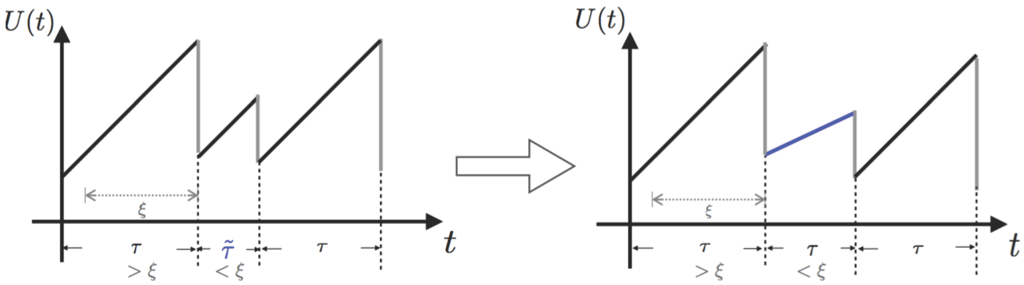
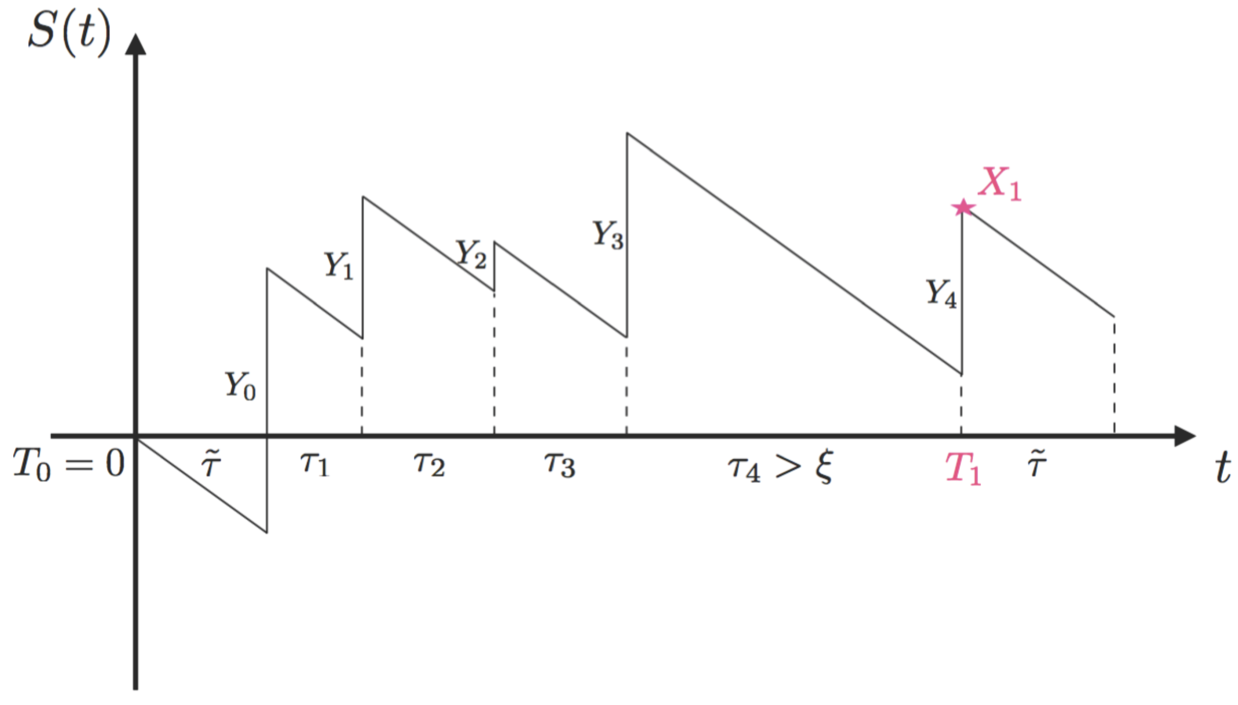
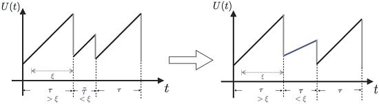
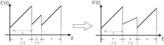
Recall our process as described by Equation (2) and note that ruin happens only at claim arrivals ${\sigma }_n={\sum }_{k=1}^n{\tau }_k$ for $n\ge 1$ and ${\sigma }_0=0$. From time ${\sigma }_n$ to ${\sigma }_{n+1}$, the distribution of the increment $S({\sigma }_{n+1})-S({\sigma }_n)$ only depends on the relation between ${\tau }_k$ and ξ. Hence, we could discretize $S(t)$ given in Equation (2) to $R_n=S({\sigma }_n)$ and, thus, transfer the model into a new one $(R_n,J_n)$ ($n\ge 0$) by adding a Markov state process ${\{J_n\}}_{n\ge 0}$ defined on $E=\{1,2\}$. The index $i\in E$ represents the occupying state of $\{J_n\}$ at time ${\sigma }_n$. For instance, State 1 describes a status where the current inter-arrival time is less than or equal to ξ, while State 2 refers to the opposite situation. For convenience, we construct ${\tau }_0$ based on the choice of $J_0$: $J_0=1$ implies ${\tau }_0\le \xi$, and ${\tau }_0>\xi$ otherwise. Note that the two-state Markov chain $\{J_n\}$ has a transition probability matrix with the $ij$-th element being $p_{ij},i,j\in E$, as follows:

$$\begin{array}{c}\hfill \mathbf{P}=\left[\begin{array}{cc}q& p\\ \tilde{q}& \tilde{p}\end{array}\right]\end{array}$$

where $p=\mathbb{P}(\tau >\xi ),q=1-p=\mathbb{P}(\tau \le \xi )$ and $\tilde{p}=\mathbb{P}(\tilde{\tau }>\xi ),\tilde{q}=1-\tilde{p}=\mathbb{P}(\tilde{\tau }\le \xi )$. We also define a new process ${\{R_n\}}_{n\ge 0}$ whose increment $\Delta R_{n+1}=R_{n+1}-R_n$ is governed by $\{J_n\}$. More specifically, two scenarios could be analysed to explain this process. Given $n=0,1,\dots$, Scenario 1 is when $J_n=1$, i.e., ${\tau }_n\le \xi$ and ${\tau }_{n+1}\stackrel{d}{=}\tau$. Then, comparing τ with ξ, there is a chance q of obtaining $J_{n+1}=1$ given $\tau \le \xi$ and p having $J_{n+1}=2$ given $\tau >\xi$, with the corresponding increment being $\Delta R_{n+1}\stackrel{d}{=}Y-{\tau }^{\le \xi }$ and $\Delta R_{n+1}\stackrel{d}{=}Y-{\tau }^{>\xi }$, respectively. On the contrary, Scenario 2 represents the situation where the current state is $J_n=2$, i.e., ${\tau }_n>\xi$ and ${\tau }_{n+1}\stackrel{d}{=}\tilde{\tau }$. Thus, all of the variables above are presented in the same way only with a tilde sign added on τ, p and q.

$Z_n=(R_n,J_n)$ is a discrete time bivariate Markov process also referred to as a discrete-time Markov additive process (MAP). The moment of ruin is the first passage time of $R_n$ over level $x>0$, defined by:

$$T^{(i)}(x)=inf\{n\in \mathbb{N}:R_n>x|Z_0=(0,i)\},\text{for}i=1,2$$

Without loss of generality, assume that ${\sigma }_{T^{(2)}(x)}=T(x)$. Then, the event $\{T^{(2)}(x)<\infty \}$ is equivalent to $\{T(x)<\infty \}$. This implies that:

$$\psi (x)=\mathbb{P}(T^{(2)}(x)<\infty )$$

To perform the simulation, we will derive now the special representation of the underlying ruin probability using a new change of measure. We start from identifying a kernel matrix $F_{ij}(dx)$ with the $ij$-th entry given by $F_{ij}(dx)={\mathbb{P}}_i(J_1=j,\Delta R_1\in dx)$. Here, ${\mathbb{P}}_i$ and ${\mathbb{E}}_i$ denote the probability measure conditional on the event $\{J_0=i\}$ and its corresponding expectation, respectively. Then, for $\theta >0$, an m.g.f of the measure $F_{ij}(dx)$ is ${\widehat{F}}_{ij}[\theta ]={\mathbb{E}}_i[{\mathrm{e}}^{\theta \Delta R_1};J_1=j]$ with:

$$\begin{array}{c}\hfill \widehat{\mathbf{F}}[\theta ]=\left[\begin{array}{cc}\mathbb{E}({\mathrm{e}}^{\theta Y}{\mathrm{e}}^{-\theta \tau };\tau \le \xi )& \mathbb{E}({\mathrm{e}}^{\theta Y}{\mathrm{e}}^{-\theta \tau };\tau >\xi )\\ \mathbb{E}({\mathrm{e}}^{\theta Y}{\mathrm{e}}^{-\theta \tilde{\tau }};\tilde{\tau }\le \xi )& \mathbb{E}({\mathrm{e}}^{\theta Y}{\mathrm{e}}^{-\theta \tilde{\tau }};\tilde{\tau }>\xi )\end{array}\right]\end{array}$$

Additionally, based on the additive structure of the process $Z_n$ for ${\widehat{F}}_{n,ij}[\theta ]={\mathbb{E}}_i[{\mathrm{e}}^{\theta (R_n-R_0)};J_n=j]$ we have,

$${\widehat{\mathbf{F}}}_n[\theta ]={(\widehat{\mathbf{F}}[\theta ])}^n$$

We will now present a few facts that will be used in the main construction.

Lemma 6. 

We have,

$${\mathbb{E}}_{J_n}[{\mathrm{e}}^{\theta (R_{n+1}-R_n)}{v}_{J_{n+1}}^{(\theta )}]=\lambda (\theta )v_{J_n}^{(\theta )}$$

(43)

where $\lambda (\theta )$ is the eigenvalue of $\widehat{\mathbf{F}}[\theta ]$ and ${\mathbf{v}}^{\theta }={(v_1^{\theta },v_2^{\theta })}^T$ is the corresponding right eigenvector.

Proof. 

Note that:

$$\begin{array}{c}\hfill {\mathbb{E}}_{J_n}[{\mathrm{e}}^{\theta (R_{n+1}-R_n)}{v}_{J_{n+1}}^{(\theta )}]={\mathbf{e}}_{J_n}^T{\widehat{\mathbf{F}}}_1[\theta ]\mathbf{v}={\mathbf{e}}_{J_n}^T\lambda (\theta )\mathbf{v}=\lambda (\theta )v_{J_n}^{(\theta )}\end{array}$$

where ${\mathbf{e}}_{J_n}$ is a standard basis vector. This completes the proof. ☐

Lemma 7. 

The following sequence:

$$L_n={\mathrm{e}}^{\theta R_n-nln\lambda (\theta )}\frac{v_{J_n}^{(\theta )}}{v_{J_0}^{(\theta )}}$$

(44)

is a discrete-time martingale.

Proof. 

Let $M_n=L_n{v}_{J_0}^{(\theta )}.$ Then,

$$\begin{array}{ccc}\hfill \mathbb{E}[M_{n+1}|{\mathcal{F}}_n]& =& \mathbb{E}[{\mathrm{e}}^{\theta R_{n+1}-(n+1)ln\lambda (\theta )}{v}_{J_{n+1}}^{(\theta )}|{\mathcal{F}}_n]\hfill \\ & =& \mathbb{E}[{\mathrm{e}}^{\theta (R_{n+1}-R_n)}{v}_{J_{n+1}}^{(\theta )}|{\mathcal{F}}_n]{\mathrm{e}}^{\theta R_n-(n+1)ln\lambda (\theta )}\hfill \\ & =& {\mathbb{E}}_{J_n}[{\mathrm{e}}^{\theta (R_{n+1}-R_n)}{v}_{J_{n+1}}^{(\theta )}]{\mathrm{e}}^{\theta R_n-(n+1)ln\lambda (\theta )}\hfill \\ & =& \lambda (\theta )v_{J_n}^{(\theta )}{\mathrm{e}}^{\theta R_n-(n+1)ln\lambda (\theta )}\hfill \\ & =& M_n\hfill \end{array}$$

which gives the assertion of the lemma. ☐

Define now a new conditional probability measure ${\mathbb{Q}}_i^{(\theta )}(dx)={\mathbb{Q}}^{(\theta )}(dx|J_0=i)$ using the Radon–Nikodym derivative as follows:

$$\frac{d{\mathbb{Q}}_i^{(\theta )}}{d{\mathbb{P}}_i}=L_n$$

Lemma 8. 

Under the new measure $\mathbb{Q}$, process ${\{Z_n^{(\theta )}\}}_{n\in \mathbb{N}}$ is again MAP specified by the Laplace transform of its kernel in the following way:

$$\begin{array}{c}\hfill {\widehat{\mathbf{F}}}^{(\theta )}[\gamma ]={\mathrm{e}}^{-ln\lambda (\theta )}{\left({\mathbf{v}}_{diag}^{(\theta )}\right)}^{-1}\widehat{\mathbf{F}}[\theta +\gamma ]{\mathbf{v}}_{diag}^{(\theta )}\end{array}$$

(45)

where ${\mathbf{v}}_{diag}^{(\theta )}$ is a diagonal matrix with ${\mathbf{v}}^{(\theta )}$ on the diagonal.

Proof. 

Note that the kernel $F_{ij}^{(\theta )}(dx)$ of $Z_n$ can be written as:

$$\begin{array}{ccc}\hfill F_{ij}^{(\theta )}(dx)& =& {\mathbb{Q}}_i^{(\theta )}(R_1\in dx,J_1=j)={\mathbb{E}}^{{\mathbb{Q}}^{(\theta )}}[{\mathbf{1}}_{\{R_1\in dx,J_1=j\}}|J_0=i]={\mathbb{E}}_i[L_1{\mathbf{1}}_{\{R_1\in dx,J_1=j\}}]\hfill \\ & =& {\mathrm{e}}^{\theta x-ln\lambda (\theta )}\frac{v_j^{(\theta )}}{v_i^{(\theta )}}{F}_{ij}(dx)\hfill \end{array}$$

This shows that the new measure is exponentially proportional to the old one, which ensures that $F_{ij}^{(\theta )}$ is absolutely continuous with respect to $F_{ij}$. Further transferring it into the matrix m.g.f. form yields the desired result. ☐

Corollary 9. 

Under the new measure ${\mathbb{Q}}^{(\theta )}$, the MAP ${\{Z_n^{(\theta )}\}}_{n\in \mathbb{N}}$ consists of a Markov state process ${\{J_n^{(\theta )}\}}_{n\in \mathbb{N}}$, which has a transition probability matrix:

$$\begin{array}{c}\hfill {\mathbf{P}}^{(\theta )}=\left[\begin{array}{cc}{q}_{\theta }& p_{\theta }\\ {\tilde{q}}_{\theta }& {\tilde{p}}_{\theta }\end{array}\right]\end{array}$$

(46)

where:

$$\begin{array}{ccc}\hfill {\tilde{p}}_{\theta }=\frac{\beta {\lambda }_2}{(\beta -\theta )({\lambda }_2+\theta )}{e}^{-({\lambda }_2+\theta )\xi },& & {\tilde{q}}_{\theta }=1-{\tilde{p}}_{\theta }\hfill \\ \hfill q_{\theta }=\frac{\beta {\lambda }_1}{(\beta -\theta )({\lambda }_1+\theta )}(1-e^{-({\lambda }_1+\theta )\xi }),& & p_{\theta }=1-q_{\theta }\hfill \end{array}$$

and an additive component ${\{R_n^{(\theta )}\}}_{n\in \mathbb{N}}$ with random variables $Y,{\tau }^{>\xi },{\tau }^{<\xi },{\tilde{\tau }}^{>\xi },{\tilde{\tau }}^{<\xi }$ with laws given in Theorem 5 where θ should be chosen everywhere instead of κ.

In fact, when $\theta =\kappa$, ${\mathbb{Q}}^{(\theta )}$ coincides with $\mathbb{Q}$ defined by Theorem 5. Recall $T^{*}(x)$ from Equation (31) and $\psi (x)\ge {\psi }^{*}(x)$. Since ${\sigma }_{T^{(2)}(x)}\le T^{*}(x)$, then $\mathbb{Q}(T^{*}(x)<\infty )=1$ implies ${\mathbb{Q}}^{(\kappa )}(T^{(2)}(x)<\infty )=1$. Now, the main representation used in simulations follows straightforwardly from the above lemmas and the optional stopping theorem, as was already done in the previous section, and it is given in the next theorem.

Theorem 10. 

The ruin probability for the underlying process Equation (2) equals:

$$\psi (x)=v_2^{(\kappa )}{e}^{-\kappa x}{\mathbb{E}}_2^{(\kappa )}\left[\frac{e^{-\kappa \epsilon (T^{(2)}(x))}}{v_{J_{T^{(2)}(x)}}^{(\kappa )}}\right]$$

(47)

where $\epsilon (T^{(2)}(x))=R_{T^{(2)}(x))}^{(\kappa )}-u$ denotes the overshoot at the time of ruin $T^{(2)}(x)$.

Proof. 

The result follows straight from Lemma 8 and Corollary 9 using the same reasoning as introduced in Section 4.1. ☐

Now, we will simulate ruin events using new parameters of the model identified in Corollary 9. We start from State 2 of $J_0$. We will run our risk process until a ruin event. With each ruin event, we will associate its weight by:

$$v_2^{(\kappa )}{e}^{-\kappa x}\frac{e^{-\kappa \epsilon (T^{(2)}(x))}}{v_{J_{T^{(2)}(x)}}^{(\kappa )}}$$

Summing and averaging all weights gives the estimate of the ruin probability $\psi (x)$.

Remark 3. 

In addition, it has been discovered that $\widehat{\mathbf{F}}[\kappa ]$ has an eigenvalue equal to one and:

$$\begin{array}{c}\hfill {\mathbf{v}}^{(\kappa )}=\left[\begin{array}{c}\frac{\beta {\lambda }_1}{(\beta -\kappa )({\lambda }_1+\kappa )}-q_{\kappa }\\ p_{\kappa }\end{array}\right]\end{array}$$

is the corresponding right eigenvector. ☐

Proof. 

Indeed, let λ denote the eigenvalue of $\widehat{\mathbf{F}}[\kappa ]$. Thus, we can write,

$$(\mathbb{E}[{\mathrm{e}}^{\kappa Y}]\mathbb{E}[{\mathrm{e}}^{-\kappa \tau },\tau \le \xi ]-\lambda )(\mathbb{E}[{\mathrm{e}}^{\kappa Y}]\mathbb{E}[{\mathrm{e}}^{-\kappa \tilde{\tau }}\tilde{\tau }>\xi ]-\lambda )={(\mathbb{E}[{\mathrm{e}}^{\kappa Y}])}^2\mathbb{E}[{\mathrm{e}}^{-\kappa \tau },\tau >\xi ]\mathbb{E}[{\mathrm{e}}^{-\kappa \tilde{\tau }},\tilde{\tau }\le \xi ]$$

Recall Equation (22); clearly, $\lambda =1$ is a solution to the above equation. That directly leads to $\widehat{\mathbf{F}}\mathbf{v}=\mathbf{v}$, and one can obtain:

$$\frac{v_1}{v_2}=\frac{\mathbb{E}[{\mathrm{e}}^{-\kappa \tau },\tau >\xi ]}{1-\mathbb{E}[{\mathrm{e}}^{-\kappa \tau },\tau \le \xi ]}$$

Plugging in the parameters completes the proof. ☐

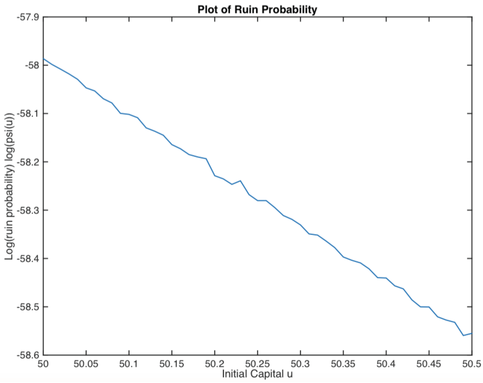
Example 2. 

Assume that Y, τ and $\tilde{\tau }$ have exponential distributions with parameters $\beta =3$, ${\lambda }_1=1$ and ${\lambda }_2=2$, respectively. The smallest positive real root of Equation (25) is calculated for $\kappa =1.1439$, and its corresponding right eigenvector is ${\mathbf{v}}^{(\mathbf{k})}={[\mathbf{0}.\mathbf{5790},\mathbf{0}.\mathbf{8153}]}^{\prime }$. Then, the ruin probability is plotted in Figure 4. It displays an exponential decay, as we expected.

4.3. Case Study

In this subsection, we derive a few results via a crude Monte Carlo simulation method. The key idea is to simulate the process according to the model setting and simply count the number of paths that get to ruin. Due to the nature of this approach, a ‘maximum’ time should be set beforehand, which means we are in fact simulating a finite time ruin probability. However, this drawback may be ignored as long as we are not getting a lot of zeros.

Our task is to compare the simulated results with a classical analytical ruin function when exponential claims are considered.

$${\psi }_C(u)=\frac{\lambda }{\beta }{\mathrm{e}}^{-(\beta -\lambda )u}$$

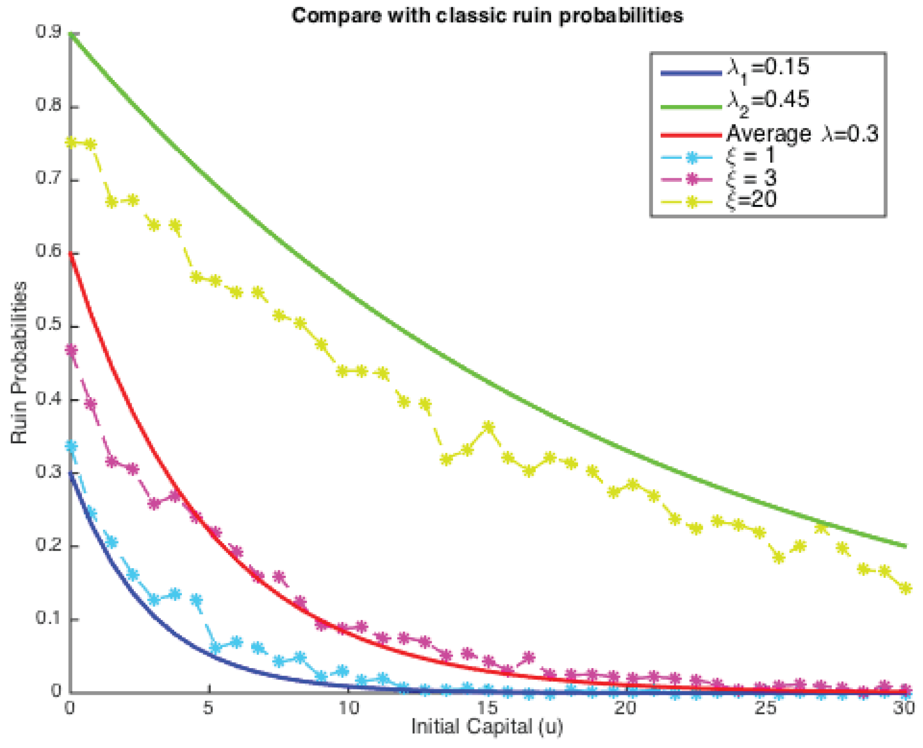
Hence, for the simplest case of exponentially-distributed claim costs, we plotted both the classic ruin probabilities and our simulated ones on the same graph, as shown below (see Figure 5).

It could be concluded that under two given parameters for Poisson intensity, simulated finite ruin probabilities in our model lie between two extremes, but have many possibilities in between. The comparison depends extensively on the value of ξ. These results also confirmed Theorem 4 that the tail of the ruin function in our case still has an exponential decay, and ξ is strongly related to the solution for κ. In other words, when the dependence is introduced, it is not clear that ruin probabilities would see an improvement.

More precisely, solid lines show classical ruin probabilities (infinite time) as a function of the initial reserve u, and each of them denotes an individual choice of Poisson parameters (${\lambda }_1=0.15$, ${\lambda }_2=0.45$) with the middle one being the average of the other two ($\lambda =0.3$). It is clear that the larger the Poisson parameter, the higher is the ruin probability. On the other hand, those dotted lines are the simulated results from our risk model with dependence for the same given pair of Poisson parameters ${\lambda }_1=0.15$ and ${\lambda }_2=0.45$. The four layers here correspond to four different choices of values for ξ, i.e., $\xi =1,\xi =3,\xi =4.44,\xi =20$. If $\xi \to 0$, the simulated ruin probability (in fact finite-time) tends to a classical case with the lower claim arrival intensities (${\lambda }_1$ here), which explains the blue dotted line lying around the dark blue solid line. On the contrary, when $\xi \to \infty$, the simulated ruin probabilities approach the other end. This then triggered us to search for a ξ, such that the simulated ruin probability coincides with a classical one. Let us see an example here, if:

$$\xi =\frac{\frac{1}{{\lambda }_1}+\frac{1}{{\lambda }_2}}{2}=4.44$$

based on the parameters we chose in Figure 5. That implies the choice of our fixed window is the average length of these two kinds of inter-arrival times. However, as can be seen from Figure 5, the dotted line with $\xi =3$ lies closer than the one with $\xi =4.44$ to the red solid line. This suggests that the choice of ξ will influence the simulated ruin probabilities and, thus, the comparison with a classical one. It is also very likely that there exists a ξ, such that our simulated ruin probabilities concur with the classic ones.

While the first half of the Monte Carlo simulation looked at the influence of ξ on the simulated ruin probabilities, the second step is to see the effects of claim sizes. The typical representations of light-tailed and heavy-tailed distributions, exponential and Pareto, were assumed for claim severities. The inter-arrival times were switching between two different exponentially-distributed random variables with parameters ${\lambda }_1$ and ${\lambda }_2$. Two cases were simulated: either ${\lambda }_1>{\lambda }_2$ or ${\lambda }_1<{\lambda }_2$. It is expected that the effects from claim severity distributions on infinite time ruin probabilities would be tiny, as they normally affect more severely the deficit at ruin. Here, since we actually simulate finite-time ruin probabilities, we are curious whether the same conclusion can be drawn.

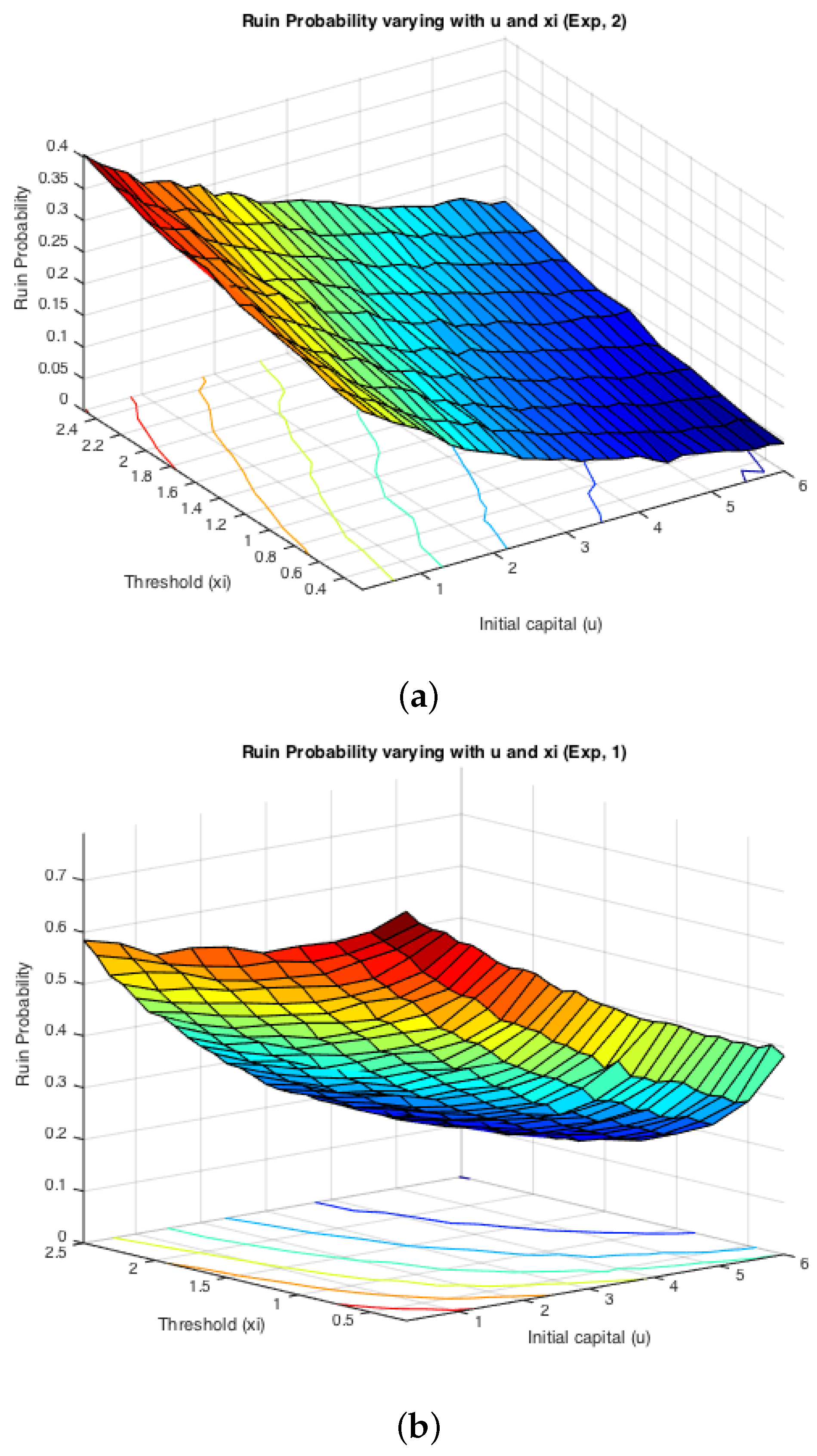
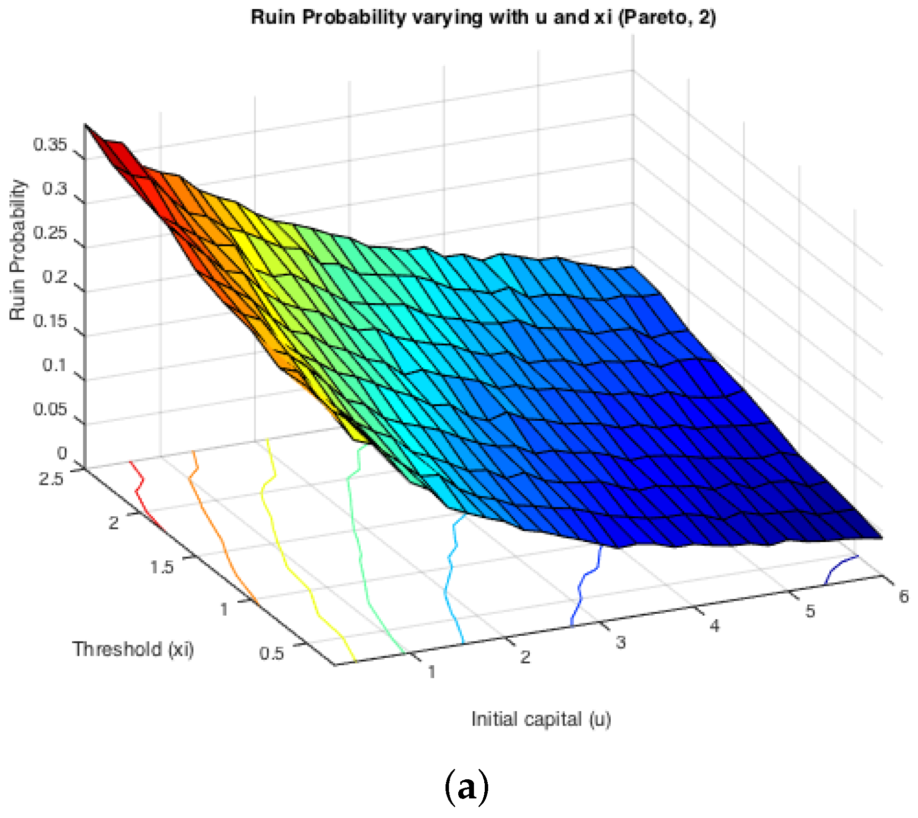
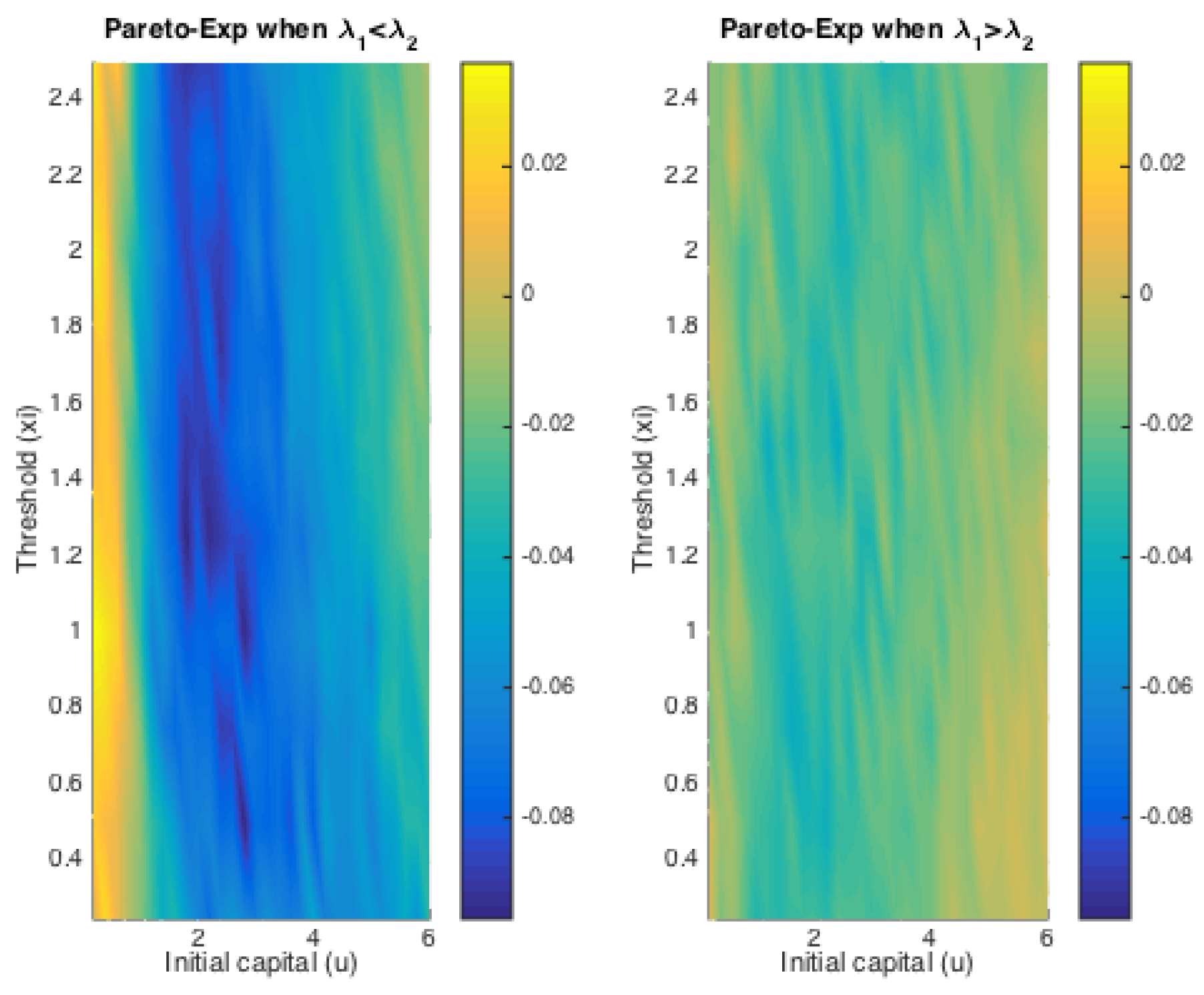
Figure 6 displays the two cases for exponential claims, while Figure 7 does that for Pareto claims. All of these four graphs demonstrate a decreasing trend for simulated finite-time ruin probabilities over the amount of initial surplus, which is as expected. In general, the differences between ruin probabilities for exponentially-distributed claim costs and those for Pareto ones are not significant. To be more precise, the exact values of these disparities are plotted in Figure 8. The color bar shows the scale of the graph, and yellow represents values around zero. Indeed, the differences are very small. Furthermore, it can be seen that the disparities behave differently when ${\lambda }_1<{\lambda }_2$ and when ${\lambda }_1>{\lambda }_2$. For the former case, ruin probabilities for Pareto claims tend to be smaller than those for exponential claims when the initial reserve is not little, whereas there seems to be no distinction between the two claim distributions in the latter case. One way to explain this is that claim distributions would have more impact on the deficit at ruin, because the claim frequency is not affected, as in an infinite-time ruin case. However, this is just a sample simulated result from which we cannot draw a general conclusion.

On the other hand, it can be seen from the projections on the $y-z$ plane that the magnitude of ${\lambda }_1$ and ${\lambda }_2$ causes different monotonicity of ruin probabilities with respect to the fixed window ξ. If ${\lambda }_1>{\lambda }_2$, the probability of ruin is monotonically increasing with the increase of ξ. 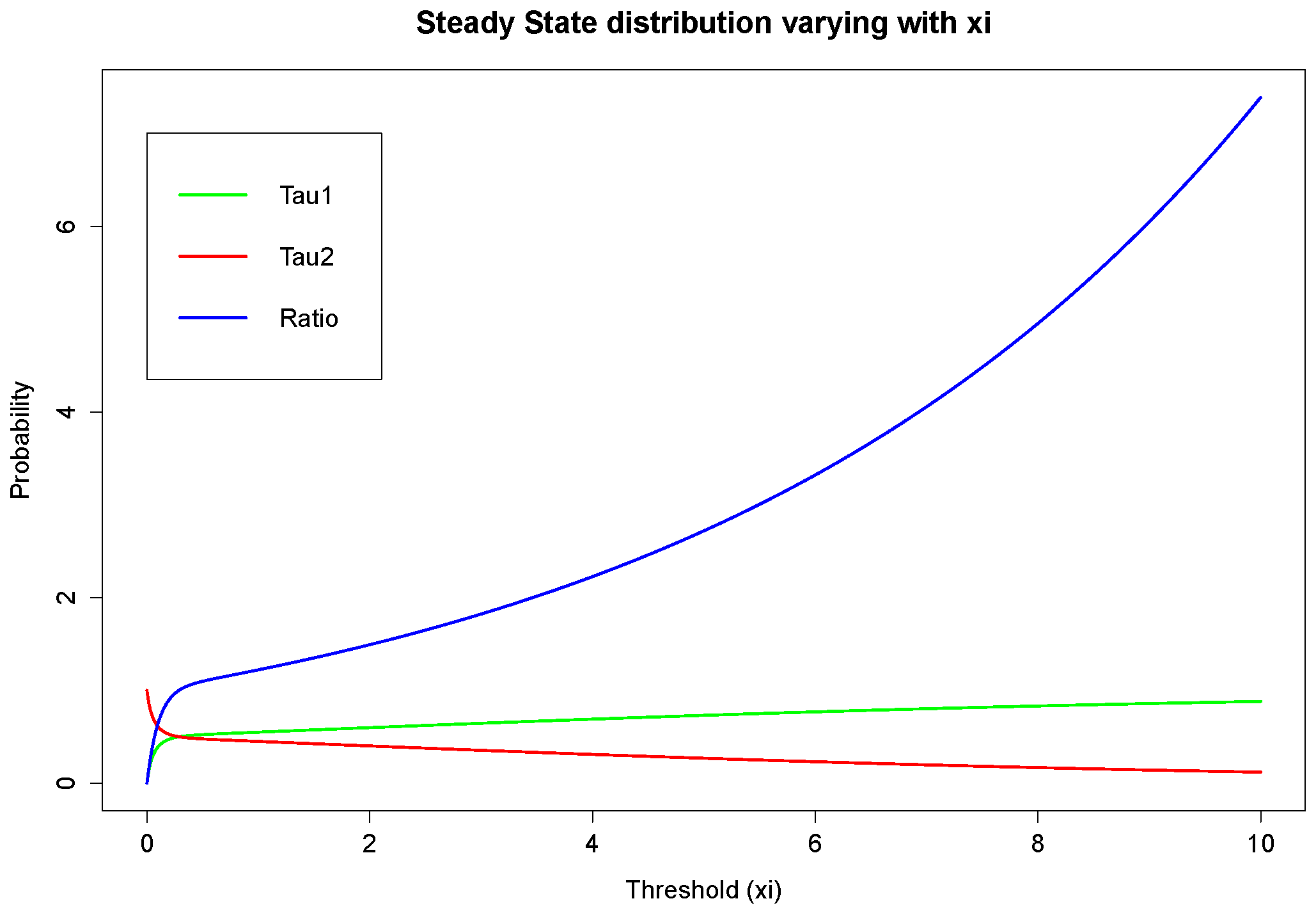If ${\lambda }_1<{\lambda }_2$, it appears to be monotonically decreasing with the rise of ξ. This conclusion for monotonicity is true for both models with heavy-tailed claims and those with light-tailed ones. Such behaviour could also be theoretically verified if we look at the stationary distribution of the Markov Chain created by the exchange of inter-claim times given by Equations (29) and (30). The increase of ξ will raise the probability of getting an inter-claim time smaller than ξ at steady state, i.e.,

$$\xi \uparrow \Rightarrow {\pi }_1\uparrow ,{\pi }_2\downarrow$$

Then, that directly leads to an increasing number of τ. Furthermore, the ruin probability is associated with:

$$S(T)=\sum _{k=1}^{N_1(T)+N_2(T)}{Y}_k-\sum _{i=1}^{N_1(T)}\tau -\sum _{j=1}^{N_2(T)}\tilde{\tau }$$

for any fixed time T, where $N_1(T)$ and $N_2(T)$ denote the number of times τ and $\tilde{\tau }$ appearing in the process. Notice that ${\sum }_{i=1}^{N_1(T)}\tau +{\sum }_{j=1}^{N_2(T)}\tilde{\tau }=T$ stays the same, even though the value of ξ alters. Therefore, now, the magnitude of $S_T$ depends only on $N_1(T)+N_2(T)$ and the distribution of i.i.d $Y_k$. The change of ξ alters only the former value. Intuitively, a rise in ${\pi }_1$ indicates an increase in $N_1(T)$ and a decrease in $N_2(T)$, whose amount is denoted by $\Delta N_1$ and $\Delta N_2$, respectively. Since the sum of τs and $\tilde{\tau }$s is kept constant, we have:

$$\begin{array}{ccc}\hfill |\Delta N_1|\mathbb{E}[\tau ]& =& |\Delta N_2|\mathbb{E}[\tilde{\tau }]\hfill \\ \hfill \left|\frac{\Delta N_1}{\Delta N_2}\right|& =& \frac{\mathbb{E}[\tilde{\tau }]}{\mathbb{E}[\tau ]}\hfill \end{array}$$

If ${\lambda }_1>{\lambda }_2$, then $\mathbb{E}[\tau ]<\mathbb{E}[\tilde{\tau }]$, which implies $\left|\frac{\Delta N_1}{\Delta N_2}\right|>1$. That is to say, the increase of $N_1(T)$ is more than the drop in $N_2(T)$, so that $N_1(T)+N_2(T)$ sees a rise in the end. Thus, it leads to a higher ruin probability. On the contrary, when ${\lambda }_1<{\lambda }_2$, i.e., $\mathbb{E}[\tau ]>\mathbb{E}[\tilde{\tau }]$, as ξ goes up, ruin probabilities would experience a monotone decay. This reasoning is visually reflected in Figure 6 and Figure 7 shown above, and it could also be noticed that the distribution of claims does not affect such monotonicity.

Therefore, by observation, these results suggest that when ${\lambda }_1<{\lambda }_2$, the larger the choice of the fixed window ξ, the smaller the ruin probability will be, and vice versa. On the contrary, when ${\lambda }_1>{\lambda }_2$, the larger the choice of the fixed window ξ, the larger the ruin probability will be, and vice versa. In fact, ${\lambda }_1<{\lambda }_2$ was mentioned in the Introduction (Figure 1) to be an assumption for a premium discount process, which resembles a bonus system. Such an observation suggests that if the insurer opts to investigate claims histories less frequently, i.e., choosing a larger ξ, the ruin probability tends to be smaller. This potentially implies a smaller ruin probability if no premium discount is offered to policyholders. It seems that to minimise an insurer’s probability of ruin probably relies more on premium incomes. The use of bonus systems may not help in decreasing such probabilities. The case of ${\lambda }_1>{\lambda }_2$ suggests an opposite conclusion for conservative insurers. This again addresses the significance of premium income to an insurer. In this situation, the ruin probability could be reduced if the insurer reviews the policyholders’ behaviours more frequently, indicating more premium incomes.

5. Conclusions

In this paper, we introduce a dependence structure within inter-arrival times into a classical insurance risk model. Precisely, the inter-arrival times switch between two random variables when compared to a fixed window ξ. Such an interchange could be equivalently converted to the change of premium rates based on recent claims, as shown by Figure 1. If the premium rates drop after a long wait, a resemblance could be drawn to a basic NCD system where there are only two classes: either a base or discounted level. Notice that the drop in premium rate is not the same as a discount for an individual in the actual NCD system, but their relation can be estimated based on a link from the individual to the collective level. However, the main goal of this paper is to study the ruin probability related to a risk model, as described in Section 2.

Several different approaches have been undertaken to study the ruin probability under the framework of a regenerative process. It is not surprising that under the Cramér assumption Equation (19), the ruin function still has an exponential tail. Since asymptotic results are not exact, we conducted numerical analyses based on different approaches. As a main contribution, we explained how we could construct a discrete Markov additive process from the model under consideration when everything is exponentially distributed. By a change of measure via exponential families, ruin probabilities were possible to simulate through a closed-form formulae Equation (47). Furthermore, we present a case study using Monte Carlo simulations. It has been shown that the underlying probability has the opposite monotonicity with respect to the fixed time window ξ when two random variables for the inter-claim times swap parameters. Additionally, it implies that the use of bonus systems may not be helpful for reducing ruin probabilities, as the premium incomes seem to be more important. However, bonus systems could still be used as a means of attracting market share, which is beneficial to the business in many ways.