
Survey on Log-Normally Distributed Market-Technical Trend Data


Institut für Mathematik, RWTH Aachen, Templergraben 55, D-52062 Aachen, Germany
*
Author to whom correspondence should be addressed.
†
These authors contributed equally to this work.
Risks 2016, 4(3), 20; https://doi.org/10.3390/risks4030020
Submission received: 5 May 2016
/
Revised: 20 June 2016
/
Accepted: 23 June 2016
/
Published: 4 July 2016
(This article belongs to the Special Issue Applying Stochastic Models in Practice: Empirics and Numerics)
Abstract
:In this survey, a short introduction of the recent discovery of log-normally-distributed market-technical trend data will be given. The results of the statistical evaluation of typical market-technical trend variables will be presented. It will be shown that the log-normal assumption fits better to empirical trend data than to daily returns of stock prices. This enables one to mathematically evaluate trading systems depending on such variables. In this manner, a basic approach to an anti-cyclic trading system will be given as an example.

1. Introduction
The concept of a trend has been fundamental in the field of technical analysis since Charles H. Dow introduced this term in the late 19th century. Following Rhea [1], Dow said, e.g., concerning the characterization of up-trends:
Successive rallies penetrating preceding high points, with ensuing declines terminating above preceding low points, offer a bullish indication.
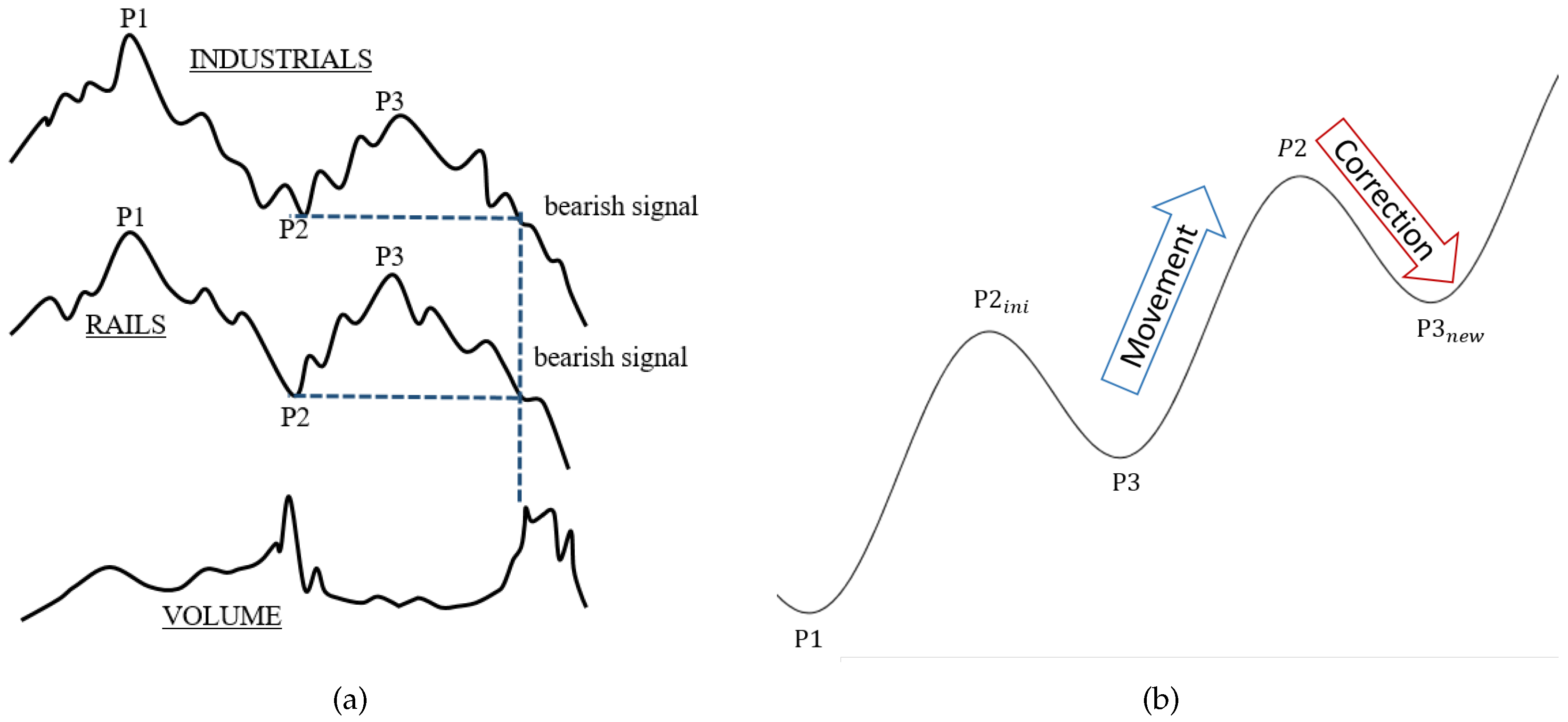
In Figure 1a, an example of the inverse situation, a down-trend, is given in a historical setup as Dow used it. Although this idea of a trend is so far “just” geometrical and clearly not precise at all, it is widely accepted among many market participants. Therefore, this geometric idea is fixed by the following market-technical definition of a Dow-trend, which is also employed in this article:
Definition 1
(market-technical trend or Dow-trend). A market is in an up-/down-trend if and only if (at least) the two last relevant lows (denoted by P1 and P3 in an up-trend) and highs (denoted by P2 in an up-trend) are monotonically increasing/decreasing (see Figure 1b). Otherwise, the market is temporarily trendless. In the case of an up-trend, the phase between a low and the next high is called the movement. In the same manner, the phase between a high and the following low is called the correction. In case of a down-trend, movement and correction are defined in the exact opposite way.
It is to analyze these Dow-trends as they occur in real-world markets within a statistical framework. In order to do so, however, a mathematical exact method on how to determine relevant lows and highs of price data is necessary.
While the task to detect the extreme points in the theoretical Figure 1b itself is trivial, it is not as easy when a real price chart is considered (see Figure 3). This can be explained by the continuous price fluctuations, and hence, the extreme points P1 − P3 are hard to detect. The issue of detection is rooted in the subjectivity of the distinction between usual fluctuations and new extreme points. This is to say: the significance of an extreme point has to be evaluated in an algorithmic way to make automatic detection possible. Therefore, referring to Maier-Paape, the framework that is necessary for automatic trend-detection will be reviewed in Section 2 [2]. The trend-detection, in turn, is rooted in the automatic recognition of relevant minima and maxima in charts. With that at hand, empirical studies of trend data can be conducted as seen in [3,4]. On the one hand, in [3], Hafizogullari, Maier-Paape and Platen collected several statistics on the performance of Dow-trends. On the other hand, in [4], Maier-Paape and Platen constructed a geometrical method on how to detect lead and lag when two markets are directly compared, also based on the automatic detection of relevant highs and lows.
In this article, however, we want to pursue a different path. We are interested in several specific trend data, such as the retracement and the relative movement and correction. Since these trend data are fundamental for the whole paper, a precise definition is given here.
The first random variable describing trend data, which will be important in the following, is the retracement denoted by X. The retracement is defined as the size-ratio of the correction and the previous movement, i.e.,
Hence, in the case of an up-trend, this is given by:
Another common random variable is the relative movement, which for an up-trend is defined by the ratio of the movement and the last low, i.e.,
and the relative correction, which for an up-trend is defined as the ratio of the correction and the last high, i.e.,
In case of a down-trend, all situations are mirrored, such that:
The main scope of this survey is to collect and extend results on how the earlier defined trend variables (plus several other related ones) can be statistically modeled. By doing this, the log-normal distribution occurs frequently. Evidently, the log-normal distribution is very well known in the field of finance. We start off, in Section 3, by giving a mathematical model of the retracement during Dow-trends and the delay of their recognition. Furthermore, the duration of the retracements and their joint distribution with the retracement will be evaluated. The results on relative movements and relative corrections during trends will be presented in Section 4. In Section 5, it will be demonstrated how the gained distributions of trend variables may be used to model trading systems mathematically.
It will be evident that the described trend data mostly fit very well to the log-normal distribution model, although there are significant aberrations for the duration of retracements (see Subsection 3.2). In the past, there have been several attempts to match the log-normal distribution model to the evolution of stock prices. It already started in 1900 with Louis Bachelier’s PhD thesis [6,7] and the approach to use the geometric Brownian motion to describe the evolution of stock prices. This yields log-normally-distributed daily returns of stock prices. Nowadays, the geometric Brownian motion is widely used to model stock prices (see [8]) especially as a part of the Black–Scholes model [9]. Nevertheless, it has to be noted that empirical studies have shown that the log-normal distribution model does not fit perfectly to daily returns (e.g., see Fama [10,11], who refers to Mandelbrot [12]).
Overall, we conclude that most of the trend data we describe fit better to the log-normal distribution model than daily returns of stock prices, although it is beyond the scope of this paper to do a formal comparison. In any case, the observed empirical facts of trend data contribute to a completely new understanding of financial markets. Furthermore, with the relatively easy calculations, which are based on the link of the log-normal distribution model to the normal distribution, complex market processes can now be discussed mathematically (e.g., with the truncated bivariate moments; see Lemma 1.21 in [13] 1).
2. Detection of Dow-Trends
The issue of automatic trend-detection has been addressed by Maier-Paape [2]. Clearly, the detection of relevant extreme points is a necessary step to detect Dow-trends. Fortunately, the algorithm introduced by Maier-Paape allows automatic detection of relevant extreme points in any market since it constructs, the so-called MinMax-processes.
Definition 2
(MinMax-process, Definition 2.6 in [2]). An alternating series of (relevant) highs and lows in a given chart is called a MinMax-process.
In Figure 3, two automatically-constructed MinMax-processes are visualized by the corresponding indicator line. The construction is based on SAR-processes (stop and reverseplease check the use of underlining throughout ).
Definition 3
(SAR-process). An indicator is called a SAR-process if it can only take two values (e.g., −1 and one, which are considered to indicate a down and an up move of the market, respectively).
Generally speaking, Maier-Paape’s algorithm looks for relevant highs when the SAR-process indicates an up move and searches for relevant lows when the SAR-process indicates a down move. Thus, the relevant extrema are “fixed” when the SAR-process changes sign. By choosing a specific SAR-process, one can affect the sensitivity of the detection while the actual detection algorithm works objectively without the need for any further parameter. For more information, see [2]. Maier-Paape also explains how to handle specific exceptional situations, for instance when a new significant low suddenly appears although the SAR-process is still indicating an up move.
It is shown by Theorem 2.13 in [2] that for any combination of SAR-process and market, there exists such a MinMax-process, which can be calculated “in real time” by the algorithm of Maier-Paape. Based on any MinMax-process in turn, it is easy to detect market-technical trends as defined in Definition 1 and then to use this information for automatic trading systems as outlined in Figure 2.
Calculating the MinMax-process “in real time” means that as time passes and the chart gets more and more candles, the extrema of the MinMax-process are constructed one by another. Besides the most recent extremum that is being searched for, all extrema found earlier are fixed from the moment of their detection, i.e., when the SAR-process changed sign.
Thus, applying the algorithm in real time also reveals some time delay in detection. Obviously, the algorithm cannot predict the future progress of the chart to which it is applied. Consequently, some delay is needed to evaluate the significance of a possible new extreme value. This circumstance is crucial when considering automatic trading systems based on market-technical trends. Therefore, it also has to affect any mathematical model of such a trading system. An approach to this issue can be made by considering the delay as an inevitable slippage. This means, not the time aspect of the delay, but more likely, the effect it has on the entry or exit price in any market-technical trading system will be evaluated. In particular, the absolute value of the delay dabs is given by:
with P[0] indicating the last detected extreme value and C[0] the close value of the current bar when this extreme value got detected.
For this article, the MinMax-process together with the integral MACD SAR-process (moving average convergence divergence; see p. 166 in [14]) was used. The integral MACD SAR (Definition 2.2 in [2]) basically is a normal MACD SAR, which in turn indicates an up move if the so-called MACD line is above the so-called signal line. Otherwise, it indicates a down move. The MACD line is given by the difference of a fast and a slow (exponential) moving average. The signal line then is an (exponential) moving average of the MACD line.
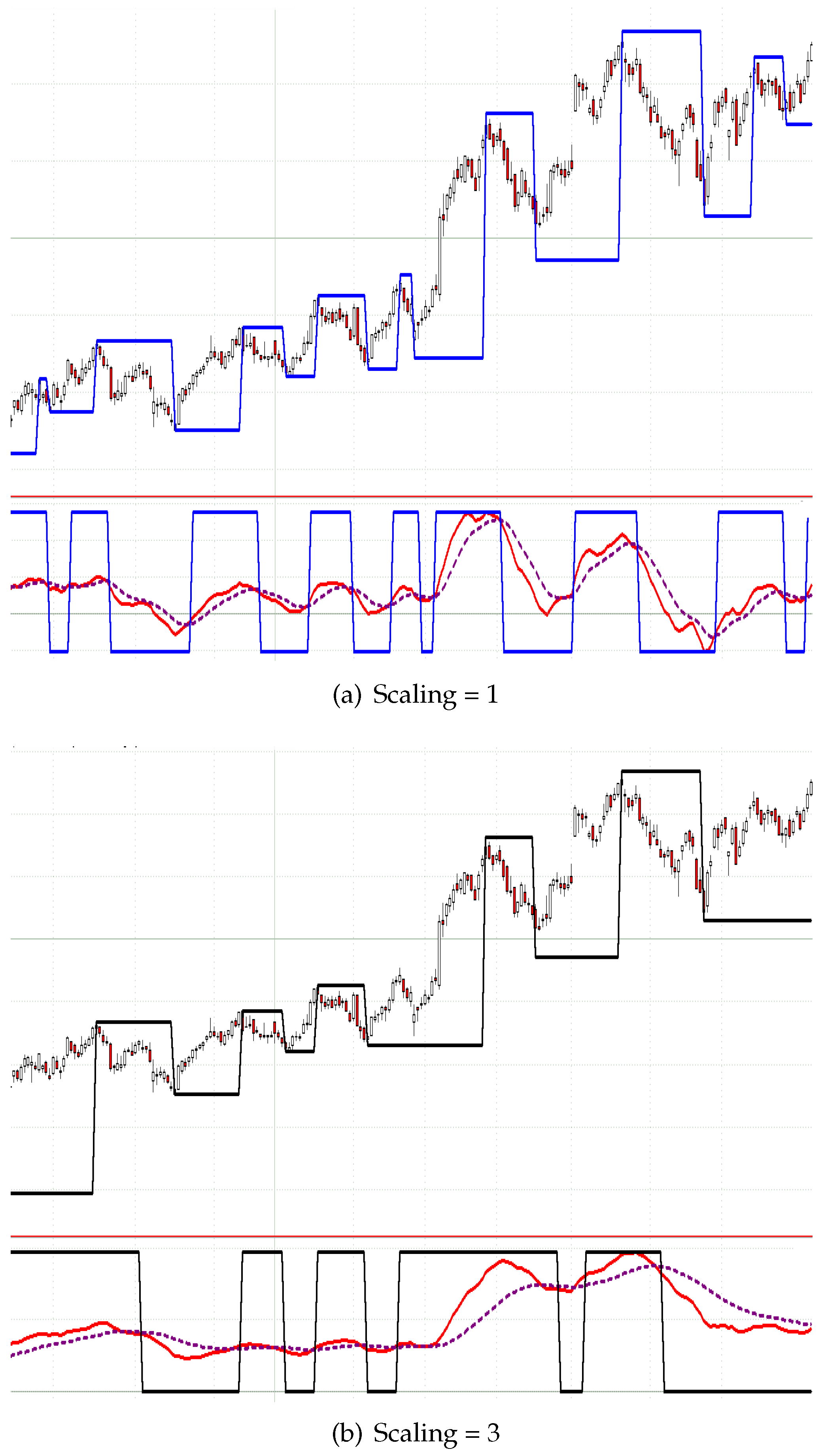
Consequently, the MACD usually takes three parameters for the fast, slow and signal line (standard values are: fast = 12, slow = 26, signal = 9). To reduce the number of needed parameters from three to one scaling parameter only, the ratios of the standard parameters are fixed and consequently scaled by the scaling parameter. In particular, an MACD with scaling parameter two denotes a usual MACD with the parameters (24/52/18). Therefore, the sensitivity of the MinMax-process solely corresponds to one scaling parameter (see Figure 3).
For a given MinMax-process, it is obvious to decide the starting and ending candle of a market-technical trend. The computation of several trend variables, such as the retracement, is therefore obvious.
The automatic detection of Dow-trends and in particular the possibility to deduce a MinMax-process out of any market given by candle data enables one to create a large dataset of empirical trend variables. The model will be based on empirical data acquired by the MinMax-process based on the integral MACD with scaling variables 1, 1.2, 1.5, 2 and 3 applied on all stocks of the current S&P100 and Eurostoxx50 in the period from January 1989 until January 2016.
3. Retracements
3.1. Distribution of the Retracement
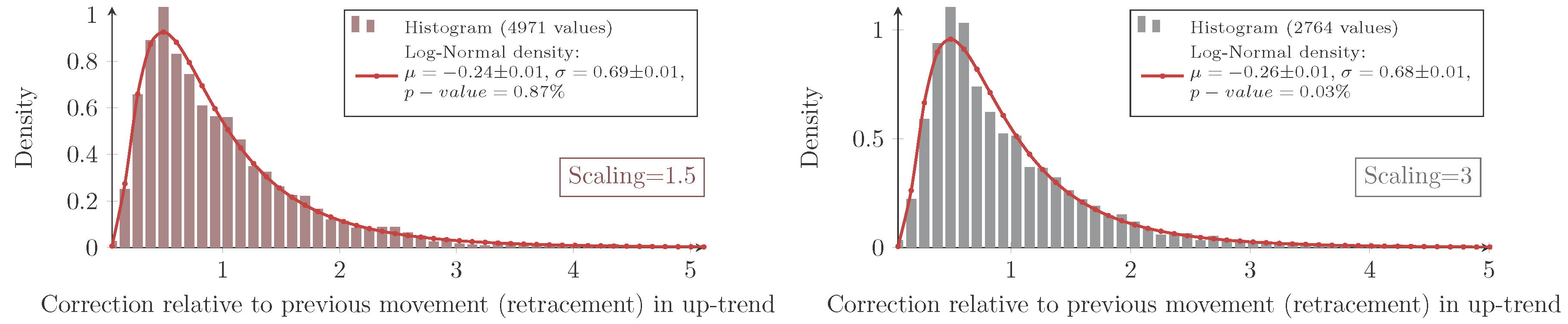
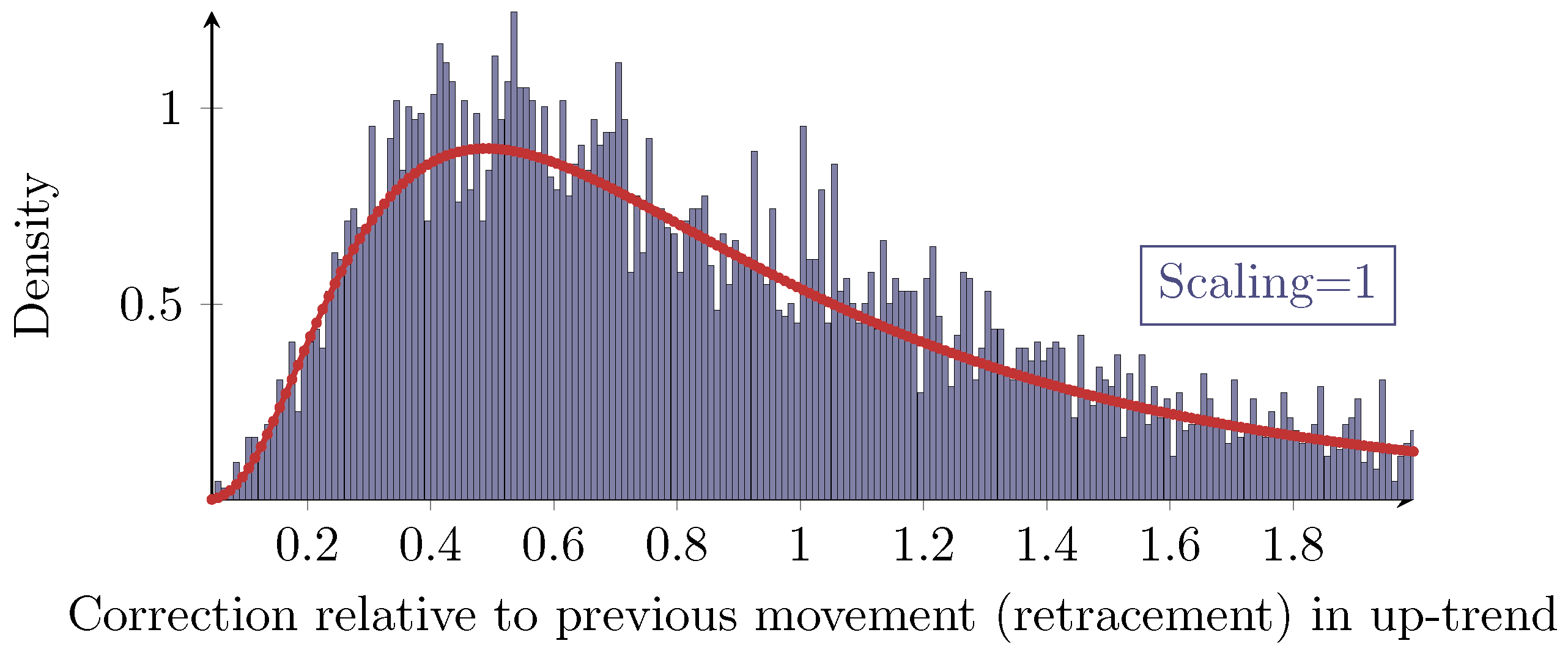
For all combinations of the regarded scalings and markets, the measured retracement data show the same characteristic distribution as seen in Figure 4 and Figure 5. Indeed, they show the typical asymmetric characteristic of a log-normal distribution, the density of which is given by:
for the retracement X and with the (true) parameters μ and σ. It is well known how to calculate moments of log-normally-distributed random variables. In this particular context, the median of the distribution X equals eμ, and the mean is given by:
To evaluate this distribution assumption, the maximum-likelihood-estimators (MLE) denoted by for the log-normal distribution are computed:
with xi denoting the n measured retracements. Furthermore, the p-value calculated with the Anderson–Darling test (recommended test by Stephens in [15], Chapter “Test based on EDF statistics”) being applied to the logarithmic transformed data is checked. The so-obtained values are summarized in Table 1.
The inconsistency of the p-values reveals that the log-normal model does not fit perfectly to the measured retracement data. In fact, all histograms show a slightly sharper density for the measured data with different intensities. Hence, for higher retracement values, the log-normal model predicts slightly fewer values than actually observed. Besides these small systematical aberrations, the log-normal model maps the measurement very well; especially for the Eurostoxx50. In addition, the log-normal model obviously fits much better to the retracement distribution than to for instance daily returns of stock prices (see Fama [10]).
To conclude the evaluation of the retracement alone, a fundamental observation about the retracement can be made (based on the log-normal assumption and the fit values derived from the data).
Observation 4
(Log-normal model for the retracement). The parameters μ and σ of the log-normal distribution are more or less scale invariant for the retracement. In the case of an up-trend, the parameters are also market invariant.
Furthermore, the parameter μ is affected by the trend direction. It is larger for down-trends, i.e., the retracements in down-trends are overall more likely to be larger than in up-trends. In spite of that, the parameter σ is more or less invariant for the trend direction.
3.2. Delay after a Retracement
As already mentioned, the delay of the MinMax-process is inevitable. Therefore, it will be evaluated in the same way as the retracement. In order to be able to compare the delay dabs after a retracement is recognized (as defined in (4)) with the retracement X itself, both must have the same unit. Therefore, the delay will also be considered in units of the last movement. It will be denoted as random variable DX:
It should be noted that (at this point), there is no statement made on whether or not DX may somehow depend on the preceding retracement X. The notation with subscript X is only used to denote the delay after a retracement and to distinguish it from other delays to come.
Again, the measured delay data show the characteristic of a log-normal distribution for each combination of scaling and market as exemplarily shown in Figure 6.
However, as expressed by the significant p-values in Table 2, the log-normal assumption lags verification.
The histograms show a systematical deviation in regard to skewness. The measured delays have a less positive skewness than predicted by the model.
Besides this systematical aberration, the log-normal model maps the characteristics precisely enough. Hence, it will be used for the following analysis.
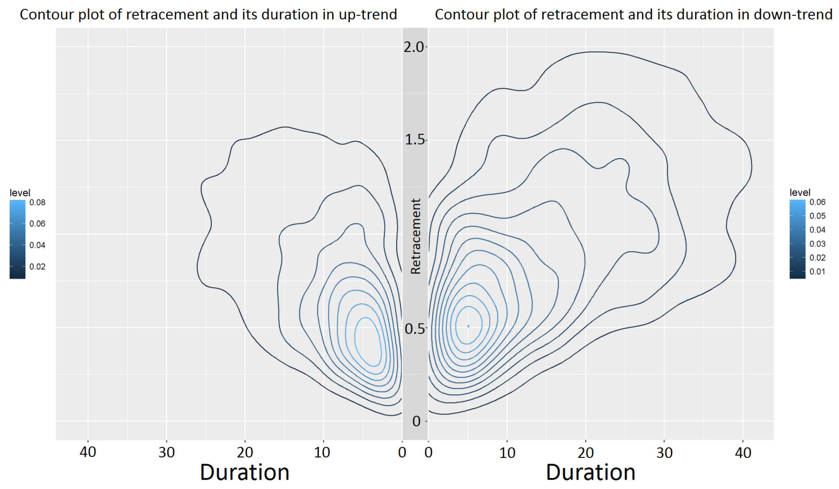
The retracement and the delay can be considered as one sequence. We therefore look for a combined log-normal distribution of retracement and delay. In this context, it is important to evaluate the estimator of the correlation ρ between the logarithm of the two variables, i.e.,
for measured values . The estimated values of are given in Table 3.
This shows that the retracement and the following delay are indeed positively correlated (regarded in the same units). This way, it is possible to give a joint bivariate log-normal distribution for the retracement X and the delay D (both in units of the preceding movement) by virtue of its density function.
For calculations based on this distribution, the (true) parameters and must be replaced by their estimators.
Finally, the concluding observation regarding the retracement can be expanded by the delay part.
Observation 5
(Log-normal model for the retracement and delay). The parameters μ and σ of the log-normal distribution are more or less scale invariant for the retracement and the delay. In the case of an up-trend, the parameters are also market invariant.
Furthermore, the parameter μ is affected by the trend direction. In the case of the retracement, it is larger for down-trends, whereas it is smaller for down-trends in the case of the delay. In spite of that, the parameter σ is more or less invariant of the trend direction.
Finally, the correlation between the logarithms of the retracement and the delay is close to scale and market invariant, while the correlation in up-trends is significantly larger than in down-trends.
3.3. Fibonacci Retracements
A propagated idea in the field of technical analysis for dealing with retracements is the concept of so-called Fibonacci retracements. Based on specific retracement levels derived from several powers of the inverse of the golden ratio, a priori predictions for future retracements shall be made. Obviously, this assumes that there are such significant retracement values. However, the evaluation of the retracement above reveals that there are no levels with a great statistical significance, but the retracements follow a continuous distribution overall. Even a finer histogram as shown in Figure 7 does not reveal any significant retracements.
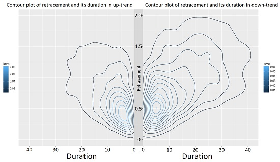
3.4. Duration of the Retracement
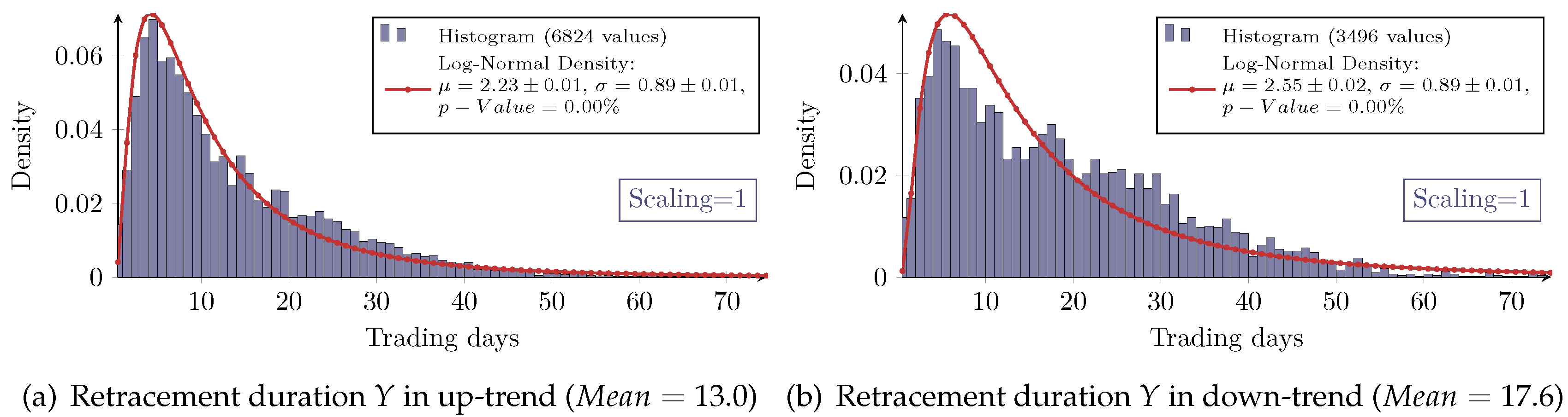
Beside the retracement, the duration of a trend correction denoted by Y is also of interest. It is given by the difference in trading days between the last P2 and the new P3 (see Figure 1b). The distributions of the retracement duration overall show the asymmetric log-normal-like behavior, as exemplarily shown in Figure 8. However, the goodness of the log-normal assumption is obviously worse as in the case of the retracement itself. In particular, the measured densities of the retracement duration in a down-trend all show significant aberrations from the log-normal model.
4. Movement and Correction
4.1. Distribution of Relative Movements and Corrections
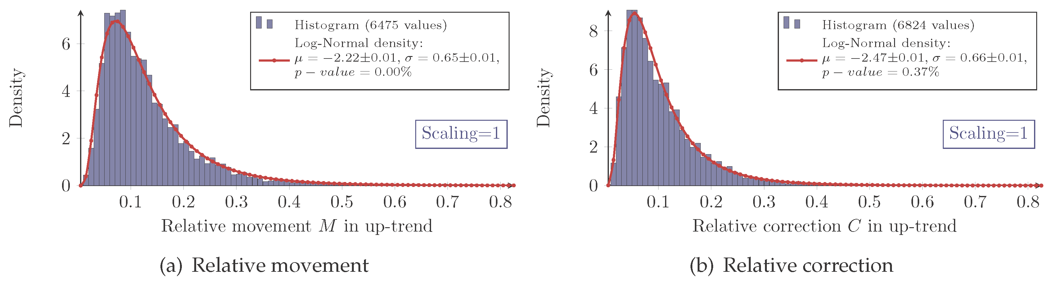
As before, all of the measurements show the same characteristic distribution, whether relative movement (2) or relative correction (3). Furthermore, the histograms conclude the log-normal assumption (see Figure 10).
Again, the log-normal model does not match the measured data perfectly. It moreover fails to map the sharp peaks and fat tails. This observation is confirmed by the fluctuating p-values (see Table 6 and Table 7).
As a consequence, based on the results of Table 6 and Table 7, a fundamental observation can be made, which differs from the retracement’s.
Observation 6
(Log-normal model for the relative movement/correction). The parameters of the log-normal distribution μ and σ are market invariant for the relative movement and correction. Furthermore, the σ parameter is more or less scale invariant while μ increases for increasing scaling for the relative movement and correction, i.e., the relative movement and correction are more likely to be larger for a higher scaling parameter.
The parameters μ and σ are also more or less trend direction invariant for the relative movement. In the case of a relative correction, however, the direction of a trend affects these parameters: both are larger in the case of a down-trend.
The dependency between the σ parameter and the scaling has already been expected as outlined above. Obviously, higher scalings yield more significant movements and corrections. Therefore, to reflect this, the x-position of the density peak has to increase when the scaling increases. The dependency of the μ parameter on the trend direction has already been observed for the retracement (see Observation 4).
4.2. Delay after Relative Movements and Corrections
As before, the delay d also has to be taken into account. Its absolute value is given by:
as defined in (4). Here, the unit for the delay is the last extreme value. This means for up-trends, the delay after the relative movement is given by:
while the delay after the relative correction is given by:
In both cases, it is sometimes abbreviated as the relative delay and has the same unit as the relative movement (2) and relative correction (3), respectively.
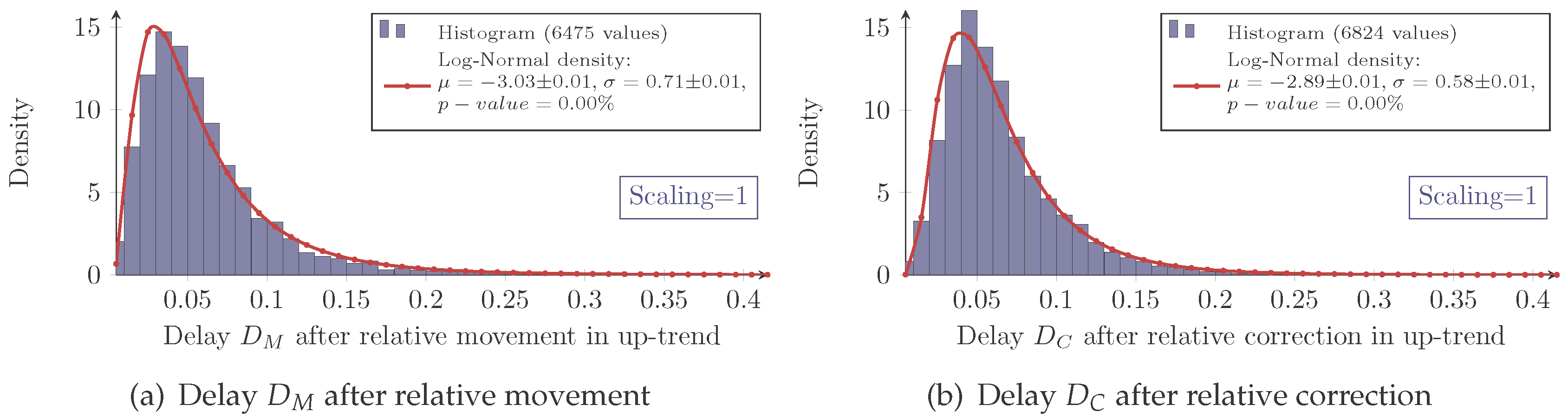
Eventually, as shown in Figure 11, the relative delay inherits the same characteristics as known from the delay for the retracement.
As before, the model’s skewness is slightly too positive. As a consequence, the same conclusion can be drawn. The model matches the measurements well enough to be the base for further analysis.
The evaluation results for the relative delay are shown in Table 8, Table 9, Table 10 and Table 11. These reveal the same behavior of the model parameters as already seen for the relative movement and correction. Furthermore, the knowledge of the correlations (Table 10 and Table 11) enables joint considerations of the relative movement/correction and the relative delay with the joint distribution (5). In sum, this leads to the following expansion of Observation 6.
Observation 7
(Log-normal model for the rel. movement/correction with delay). The parameters of the log-normal distribution μ and σ are market invariant for the relative movement and correction, as well as their corresponding relative delays. Additionally, for these trend variables, the σ parameter is more or less scale invariant while μ increases for increasing scaling.
The parameters μ and σ are also more or less trend direction invariant for the relative movement (Table 6). In the case of the relative correction, however, the direction of a trend affects these parameters: both are larger in the case of a down-trend (Table 7). This is also true for the relative delay after a correction (Table 9). For the relative delay after a movement, μ is also larger, whereas σ is smaller for down-trends (Table 8).
Finally, the correlation between the logarithms of the relative movement/correction and the corresponding relative delay is close to scale invariant.
4.3. Period of Movements and Corrections
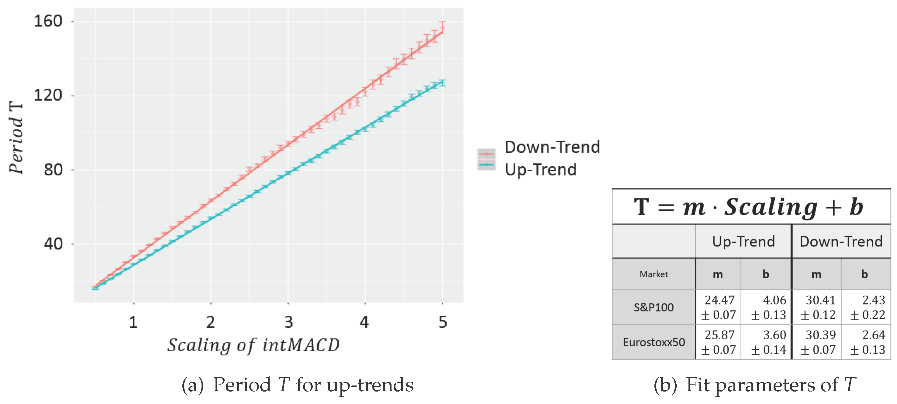
The dependency between μ and the scaling parameter has already been explained with their connection to the level of trend significance (Observation 6). One attribute of trend significance is the duration of a single trend period. Hence, the time difference between two lows and two highs within the up- and down-trend, respectively, is called the period T of a trend. Figure 12a shows the evolution of T regarding different scaling parameters. For any scaling, the T value is the arithmetical mean of all time differences between two consecutive lows and highs within up- and down-trends, respectively.
The period T shows a linear behavior, which has already been observed in [3] for EUR-USD charts. The fit parameters are similar for both evaluated markets, but differ in regard to the type of trend (see Figure 12b). Due to the linear model, it is evident how to set the scaling parameter in order to emphasize a specific period. Consequently, it is also obvious to map any of the three different trend classes introduced by Dow; namely the primary, secondary and tertiary trend (see Murphy, chapter “Dow Theory” in [17]).
5. Mathematical Model of Trading Systems
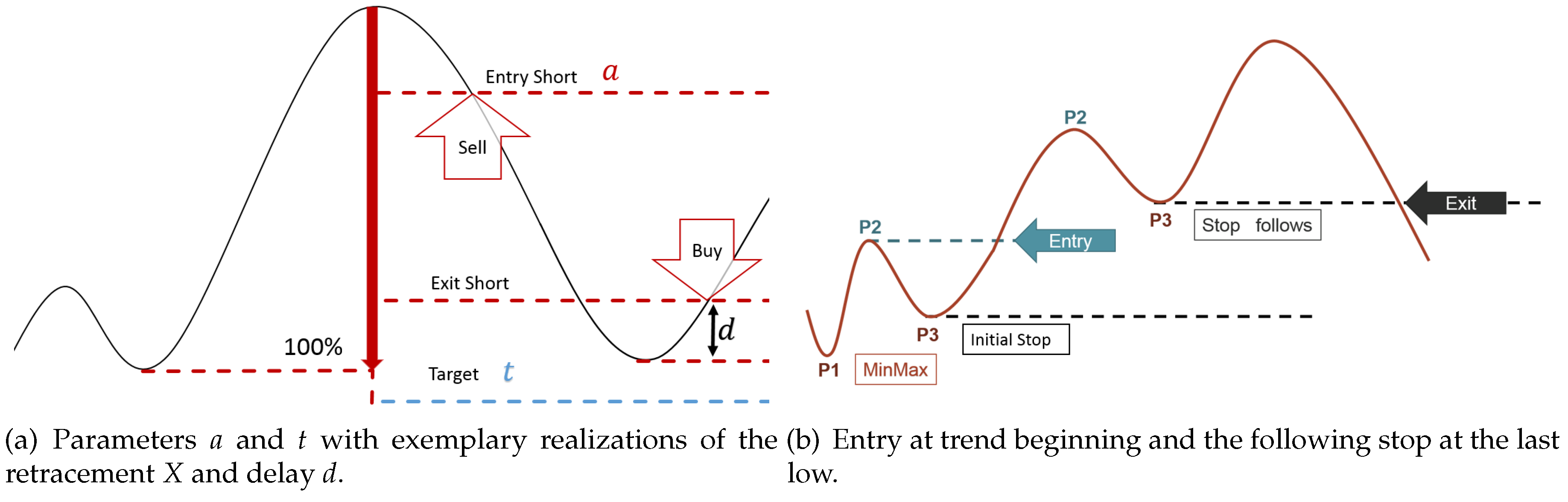
Based on the log-normal distribution model of the retracement, an anti-cyclic trading system can be modeled, for instance. With the joint density of the retracement and delay, the return of a basic anti-cyclic trading system as shown in Figure 13 can be calculated:
Lemma 8
(Expected return). Let an anti-cyclic trading system as shown in Figure 13a with entry in the correction at retracement level a, target t, be given. As soon as the end of the correction is recognized, the position is closed with delay d. Furthermore, the return (in units of the last movement) for a trade with retracement x and delay d denoted by is given by:
Moreover, the distribution of the random variable for the retracement X and for the delay after the the retracement are known from Section 3. That is the reason why the expected value of this return, considering only retracements where the trade is opened (condition ), is given by:
with denoting the distribution function of the retracement X (see Section 3).
It should be noted that a and t are parameters that have to be given in the same units as the retracement, i.e., units of the last movement.
In the same manner, several other key figures, such as the variance of the return, can be calculated analytically when assuming the empirically-observed distributions as real. In this way, an unfavorable chance to the risk ratio for the anti-cyclic trading model has been revealed (see [13]3). This is, however, in accordance with the empirical observations of the strategy’s backtests.
6. Conclusions and Outlook
In this survey, the applications of the log-normal distribution model on market-technical trend data is introduced. On the one hand, it is remarkable that the log-normal model fits better to the trend data presented than to daily returns of stock prices. In contrast to the approach on the latter, however, there has not been found any explanation for this observation yet. In particular, it has not yet been clarified whether the log-normal distribution is a result of a limit process or can be explained with the log-normal model for the daily returns of stock prices. As far as applications in the direction of modeling of trading systems are concerned, we introduced a simple model for an anti-cyclic trading setup based on log-normally distributed data.
On the other hand, trend following, i.e., pro-cyclic trading systems, are more widely used than anti-cyclic ones. In fact, empirical backtests have already shown the profitability of such trading systems. Consequently, there is a need for a mathematical model. Unfortunately, pro-cyclic trading usually implies holding a position over several iterations of movement and correction as outlined in Figure 13b.
This makes the problem far more complicated in mathematical terms since the joint distribution of a random number of relative movements and corrections, with possible correlations, has to be considered. Nevertheless, the log-normal model for the trend data represents a promising approach to this issue, as well.
Author Contributions
R. Brenner and S. Maier-Paape contributed equally to this work.
Conflicts of Interest
The authors declare no conflict of interest.
References
- R. Rhea. The Dow Theory. Flint Hill, VA, USA: Fraser Publishing Company, 1993. [Google Scholar]
- S. Maier-Paape. “Automatic one two three.” Quant. Finance 15 (2015): 247–260. [Google Scholar] [CrossRef]
- Y. Hafizogullari, S. Maier-Paape, and A. Platen. Empirical Study of the 1-2-3 Trend Indicator. Report No. 61; Nordrhein-Westfalen, Geramny: Institute for Mathematics, RWTH Aachen, 2013, p. 21. [Google Scholar]
- S. Maier-Paape, and A. Platen. Lead-Lag Relationship Using a Stop-and-Reverse-MinMax Process. Report No. 79; Nordrhein-Westfalen, Geramny: Institute for Mathematics, RWTH Aachen, 2015, p. 22. [Google Scholar]
- R. Russell. Dow Theory Today. Thousand Oaks, CA, USA: Snowball Publishing, 1961. [Google Scholar]
- L. Bachelier. “Theorie de la Speculation.” Ph.D. Thesis, University of Paris, Paris, France, 1900. [Google Scholar]
- P.H. Cootner, ed. The Random Character of Stock Market Prices. Cambridge, MA, USA: MIT Press, 1964, pp. 17–75.
- J. Hull. Options, Futures, and other Derivatives, 7th ed. Upper Saddle River, NJ, USA: Prentice Hall, 2009. [Google Scholar]
- F. Black, and M. Scholes. “The pricing of options and corporate liabilities.” J. Polit. Econ. 81 (1973): 637–654. [Google Scholar] [CrossRef]
- E.F. Fama. “Mandelbrot and the stable paretian hypothesis.” J. Bus. 36 (1963): 420–429. [Google Scholar] [CrossRef]
- E.F. Fama. “The behavior of stock-market prices.” J. Bus. 38 (1965): 34–105. [Google Scholar] [CrossRef]
- B. Mandelbrot. “The variation of certain speculative prices.” J. Bus. 36 (1963): 394–419. [Google Scholar] [CrossRef]
- R. Kempen. “Mathematical Modeling of Movement and Correction Trading with Log-Normal Distribution Ansatz.” Master’s Thesis, RWTH Aachen University, Nordrhein-Westfalen, Geramny, 2015. [Google Scholar]
- G. Appel. Technical Analysis: Power Tools for Active Investors. Harlow Essex, UK: Financial Times Prentice Hall, 2005. [Google Scholar]
- R.B. D’Agostino, and M.A. Stephens. Goodness-of-Fit Techniques. New York, NY, USA: Marcel Dekker, 1986. [Google Scholar]
- R. Kempen. “Fibonaccis are human (made).” IFTA J., 2016, 4–9. [Google Scholar]
- J.J. Murphy. Technical Analysis of the Financial Markets. New York, NY, USA: New York Institute of Finance, 1999. [Google Scholar]
- 1.Published under R. Brenner’s birth name Kempen.
- 2.Published under R. Brenner’s birth name Kempen.
- 3.Published under R. Brenner’s birth name Kempen.
Figure 1.
(a) Example of a down-trend in a historical setup as Dow used it (freely adapted from Russel [5]); (b) sketch of an up-trend in the sense of Dow.
Figure 1.
(a) Example of a down-trend in a historical setup as Dow used it (freely adapted from Russel [5]); (b) sketch of an up-trend in the sense of Dow.

Figure 2.
General concept of the automatic detection of Dow-trends.
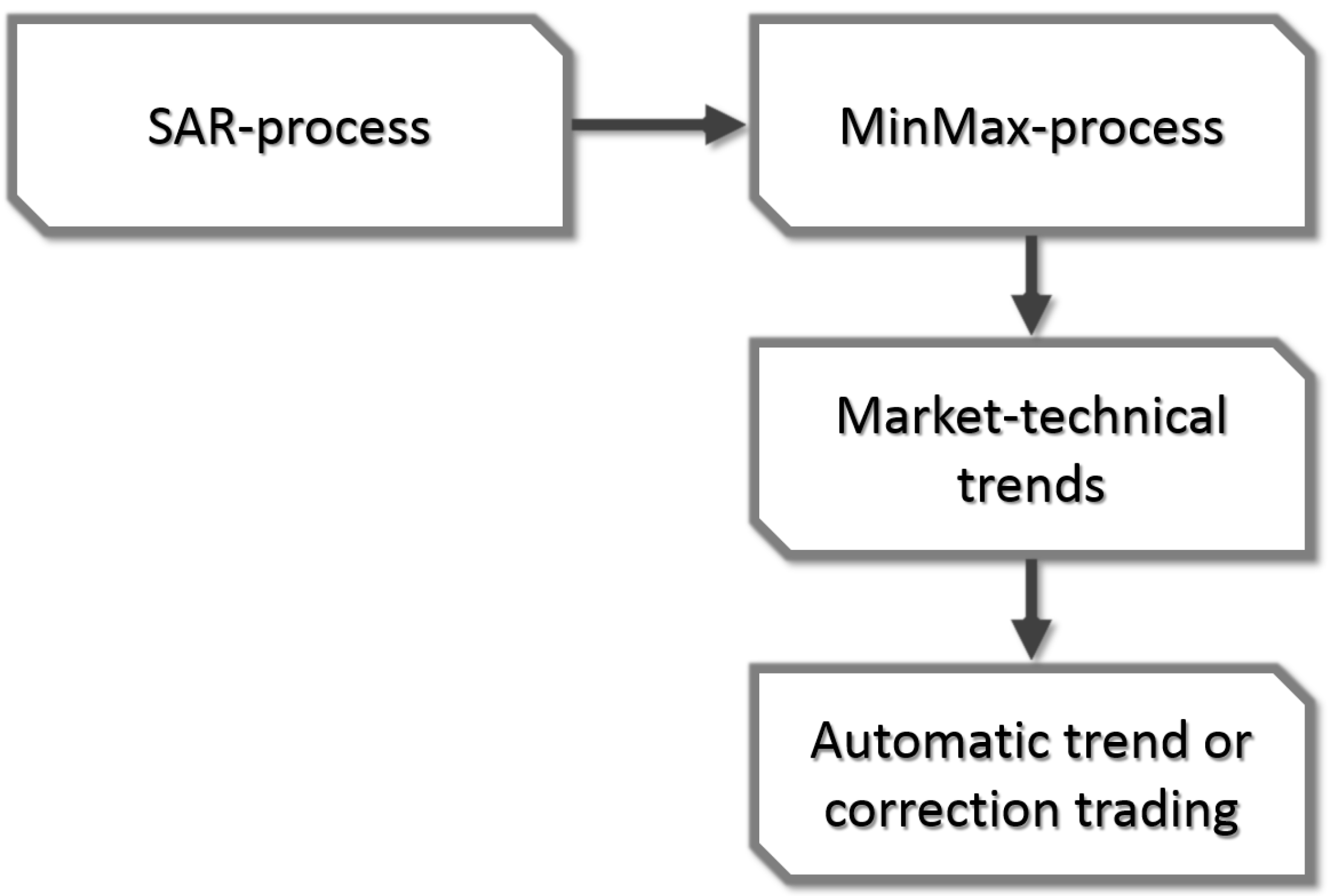
Figure 3.
Daily chart of the Adidas stock between September 2012 and August 2013 with the MinMax-process by Maier-Paape (a) based on the integral moving average convergence divergence (MACD) stop and reverse (SAR)-process (b) with two different scalings: one and three. The lines in the charts indicate the last detected extremum.

Figure 4.
Measured and log-normal fit density of the retracement X in an up-trend and down-trend with scaling one for S&P100 stocks. Each dataset is visualized with a histogram from zero to five with a bin size of 0.11.
Figure 4.
Measured and log-normal fit density of the retracement X in an up-trend and down-trend with scaling one for S&P100 stocks. Each dataset is visualized with a histogram from zero to five with a bin size of 0.11.
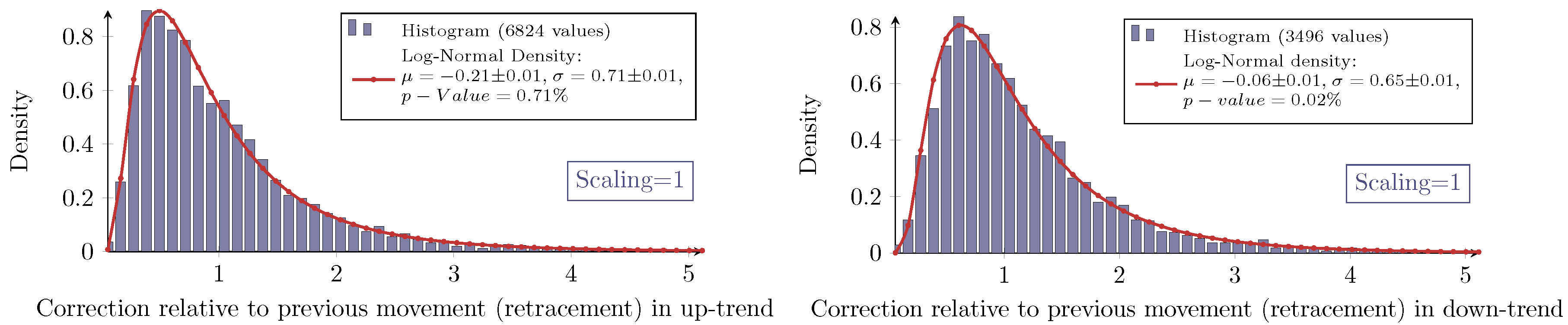
Figure 5.
Measured and log-normal fit density of the retracement X in an up-trend with scaling 1.5 and three for S&P100 stocks. Each dataset is visualized with a histogram from zero to five with a bin size of 0.11.
Figure 5.
Measured and log-normal fit density of the retracement X in an up-trend with scaling 1.5 and three for S&P100 stocks. Each dataset is visualized with a histogram from zero to five with a bin size of 0.11.

Figure 6.
Measured and log-normal fit density of the delay in an up-trend with scaling one for S&P100 stocks. The data are visualized with a histogram from zero to five with a bin size of 0.11.
Figure 6.
Measured and log-normal fit density of the delay in an up-trend with scaling one for S&P100 stocks. The data are visualized with a histogram from zero to five with a bin size of 0.11.
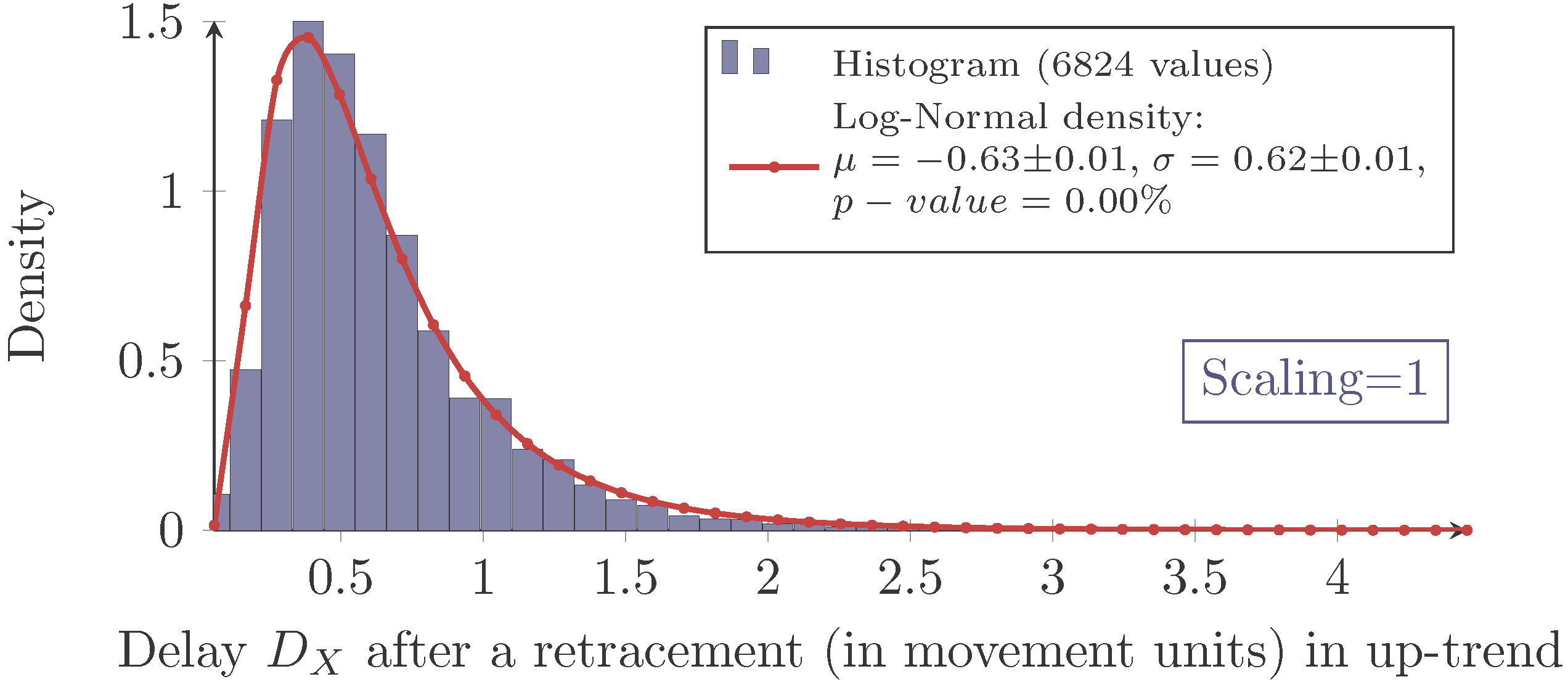
Figure 7.
More detailed (finer) histogram of Figure 4 with scaling one from zero to two with a bin size of 0.01.
Figure 7.
More detailed (finer) histogram of Figure 4 with scaling one from zero to two with a bin size of 0.01.

Figure 8.
Measured and log-normal fit density of the retracement duration in up- and down-trends (a and b respectively) with scaling one for S&P100 stocks. The data are visualized with a histogram with a bin size of one.
Figure 8.
Measured and log-normal fit density of the retracement duration in up- and down-trends (a and b respectively) with scaling one for S&P100 stocks. The data are visualized with a histogram with a bin size of one.

Figure 9.
Contour plot of the joint density of the retracement value and its duration in up- and down-trends (left and right resp.) with scaling one for S&P100 stocks.
Figure 9.
Contour plot of the joint density of the retracement value and its duration in up- and down-trends (left and right resp.) with scaling one for S&P100 stocks.

Figure 10.
Measured and log-normal fit density of the relative movement (a) and relative correction (b) in an up-trend with scaling one for S&P100 stocks. The data are visualized via histogram from zero to one with a bin size of 0.01.
Figure 10.
Measured and log-normal fit density of the relative movement (a) and relative correction (b) in an up-trend with scaling one for S&P100 stocks. The data are visualized via histogram from zero to one with a bin size of 0.01.

Figure 11.
(a) Measured and log-normal fit density of the relative delay after a relative movement M (see 2) and (b) after a relative correction C (see 3) in an up-trend with scaling one for S&P100 stocks. The data are visualized with a histogram from zero to one with a bin size of 0.01.
Figure 11.
(a) Measured and log-normal fit density of the relative delay after a relative movement M (see 2) and (b) after a relative correction C (see 3) in an up-trend with scaling one for S&P100 stocks. The data are visualized with a histogram from zero to one with a bin size of 0.01.

Figure 12.
Evolution of the period T for scalings between 0.5 and five with a step size of 0.1 for S&P100 stocks. (a) period T for up-trends. (b) Fit parameters of T.
Figure 12.
Evolution of the period T for scalings between 0.5 and five with a step size of 0.1 for S&P100 stocks. (a) period T for up-trends. (b) Fit parameters of T.

Figure 13.
Setup of a basic anti- and pro-cyclic trading system for up-trends (a and b, respectively).
Figure 13.
Setup of a basic anti- and pro-cyclic trading system for up-trends (a and b, respectively).

Table 1.
Parameters of the log-normal fit for the retracement X in up- and down-trends. (a) S&P100 data. (b) Eurostoxx50 data.
Table 1.
Parameters of the log-normal fit for the retracement X in up- and down-trends. (a) S&P100 data. (b) Eurostoxx50 data.

Table 2.
Parameters of the log-normal fit for the delay DX in up- and down-trends. (a) S&P100 data. (b) Eurostoxx50 data.
Table 2.
Parameters of the log-normal fit for the delay DX in up- and down-trends. (a) S&P100 data. (b) Eurostoxx50 data.

Table 3.
Correlation between the logarithms of the retracement X (retr.) and delay DX (after retr.) in up- and down-trends. (a) S&P100 data. (b) Eurostoxx50 data.
Table 3.
Correlation between the logarithms of the retracement X (retr.) and delay DX (after retr.) in up- and down-trends. (a) S&P100 data. (b) Eurostoxx50 data.

Table 4.
Parameters of the log-normal fit for the retracement duration in up- and down-trends. (a) S&P100 data. (b) Eurostoxx50 data.
Table 4.
Parameters of the log-normal fit for the retracement duration in up- and down-trends. (a) S&P100 data. (b) Eurostoxx50 data.

Table 5.
Correlation between the logarithms of the retracement X (retr.) and its duration Y in up- and down-trends. (a) S&P100 data. (b) Eurostoxx50 data.
Table 5.
Correlation between the logarithms of the retracement X (retr.) and its duration Y in up- and down-trends. (a) S&P100 data. (b) Eurostoxx50 data.

Table 6.
Parameters of the log-normal fit for the relative movement in up- and down-trends. (a) S&P100 data. (b) Eurostoxx50 data.
Table 6.
Parameters of the log-normal fit for the relative movement in up- and down-trends. (a) S&P100 data. (b) Eurostoxx50 data.

Table 7.
Parameters of the log-normal fit for the relative correction in up- and down-trends. (a) S&P100 data. (b) Eurostoxx50 data.
Table 7.
Parameters of the log-normal fit for the relative correction in up- and down-trends. (a) S&P100 data. (b) Eurostoxx50 data.

Table 8.
Parameters of the log-normal fit for the relative delay DM after a movement in up- and down-trends. (a) S&P100 data. (b) Eurostoxx50 data.
Table 8.
Parameters of the log-normal fit for the relative delay DM after a movement in up- and down-trends. (a) S&P100 data. (b) Eurostoxx50 data.

Table 9.
Parameters of the log-normal fit for the relative delay DC after a correction in up- and down-trends. (a) S&P100 data. (b) Eurostoxx50 data.
Table 9.
Parameters of the log-normal fit for the relative delay DC after a correction in up- and down-trends. (a) S&P100 data. (b) Eurostoxx50 data.

Table 10.
Correlation between the logarithms of the relative (rel.) movement M and relative delay DM in up- and down-trends. (a) S&P100 data. (b) Eurostoxx50 data.
Table 10.
Correlation between the logarithms of the relative (rel.) movement M and relative delay DM in up- and down-trends. (a) S&P100 data. (b) Eurostoxx50 data.

Table 11.
Correlation between the logarithms of the relative (rel.) correction C and relative delay DC in up- and down-trends. (a) S&P100 data. (b) Eurostoxx50 data.
Table 11.
Correlation between the logarithms of the relative (rel.) correction C and relative delay DC in up- and down-trends. (a) S&P100 data. (b) Eurostoxx50 data.

© 2016 by the authors; licensee MDPI, Basel, Switzerland. This article is an open access article distributed under the terms and conditions of the Creative Commons Attribution (CC-BY) license (http://creativecommons.org/licenses/by/4.0/).
Share and Cite
MDPI and ACS Style
Brenner, R.; Maier-Paape, S. Survey on Log-Normally Distributed Market-Technical Trend Data. Risks 2016, 4, 20. https://doi.org/10.3390/risks4030020
AMA Style
Brenner R, Maier-Paape S. Survey on Log-Normally Distributed Market-Technical Trend Data. Risks. 2016; 4(3):20. https://doi.org/10.3390/risks4030020
Chicago/Turabian StyleBrenner, René, and Stanislaus Maier-Paape. 2016. "Survey on Log-Normally Distributed Market-Technical Trend Data" Risks 4, no. 3: 20. https://doi.org/10.3390/risks4030020
Note that from the first issue of 2016, this journal uses article numbers instead of page numbers. See further details here.