
A Note on the Impact of Parameter Uncertainty on Barrier Derivatives


1
Western University, London, ON N6A 3K7, Canada
2
Chair of e-Finance, Goethe University Frankfurt, D-60323 Frankfurt am Main, Germany
*
Author to whom correspondence should be addressed.
Risks 2016, 4(4), 35; https://doi.org/10.3390/risks4040035
Submission received: 31 August 2016
/
Revised: 31 August 2016
/
Accepted: 21 September 2016
/
Published: 29 September 2016
Abstract
:This paper presents a comprehensive extension of pricing two-dimensional derivatives depending on two barrier constraints. We assume randomness on the covariance matrix as a way of generalizing. We analyse common barrier derivatives, enabling us to study parameter uncertainty and the risk related to the estimation procedure (estimation risk). In particular, we use the distribution of empirical parameters from IBM and EURO STOXX50. The evidence suggests that estimation risk should not be neglected in the context of multidimensional barrier derivatives, as it could cause price differences of up to 70%.
1. Introduction
It is a well-established fact that both volatility and correlation play significant roles in modelling financial markets. For instance, volatility is crucially important in asset pricing models and dynamic hedging strategies, as well as in the determination of option prices. Besides financial derivative specifications, such as maturity and the strike price, volatility is the most influential parameter and the most difficult to quantify. Similarly, correlations play a vital role in the market and its derivatives. However, since the correlation meltdown during the financial crisis in 2008, where all correlations were moving close to one altogether, people have been more aware of the importance of correlation and vanishing diversification effects, not only for risk management, but also for multi-asset derivatives.
Consequently, and unlike the other specifications, volatility, as well as correlation have to be modelled as time-dependent processes. The best solution to this challenge is a stochastic covariance model, as those stochastic matrices tackle both features, volatility and correlation, simultaneously (see [1,2,3]). In such a context, when it comes to the actual pricing of products, practitioners either determine model parameters from option prices (usually called calibration) or obtain the parameters from historical observations of the underlying (estimation methodology). The first approach has plenty of limitations; for instance, the correlation can not be ‘implied’ due to a lack of freely-tradable multivariate derivatives; hence, one has to incorporate hidden processes into the calibration methodology, leading to high non-linearity. This makes the calibration unstable numerically. On the other hand, the second approach requires plenty of data points even though these parameters may not remain constant for long periods. Moreover, stochastic covariance models suffer from higher complexity, which is particularly problematic for path-dependent products like barrier options. The pricing of these products is nowadays unfeasible in stochastic covariance models. In a nutshell, stochastic covariance models do not lead to an analytical solution or numerically-feasible methods for the pricing of path-dependent derivatives (see [4] for a discussion).
This takes us back to the constant covariance case, the Black–Scholes framework. Although we have seen already that this assumption does not capture empirical observations, it also fails to incorporate a second fact: the parameters are unknown. In other words, when using sample data, one deals with point estimates instead of the true value of the parameters. A rigorous approach should work with the point estimator instead of the actual estimate. Point estimators are random variables that would account for the uncertainty related to the estimation procedure. In most cases, point estimates are extremely sensitive to small changes in the estimation procedure (maximum likelihood versus a Bayesian approach), the number of data observations (large versus small sample sizes) or the type of parameter (e.g., mean versus variance); and in general, the distribution of the point estimator is not known in closed form (i.e., it does not belong to a known family of distributions). This analysis is called estimation risk, as it describes the risk or the inaccuracy related to substituting the sample estimate for the true unknown parameters.
Estimation risk was considered very early in the seminal work of [5], which finds little impact on simple European-type option prices. On the other hand, Lence, S.H. et al. [6] detected a significant impact on portfolio allocation. More recently, Jacquier, E. et al. [7] shows the importance of estimation risk in model assessment for general contingency claims in a one-dimensional setting using a Bayesian approach. The work in [8] deals with non-path-dependent one-dimensional option prices to assess the estimation risk with similar findings. Nevertheless very little has been done to assess estimation risk for path-dependent products, in particular the most popular barrier options. One possible reason for this lack of analysis in the literature is the difficulties in finding closed-form solutions for barrier products. The work of [9] pioneered closed-form expressions in the presence of one barrier, while [1] provided the framework to price analytically options with two barriers. More recently, the limitations on analytical expressions for more than two barriers were highlighted in the work of [10] (three barriers) and [11] (more than three). All previous findings were in a constant covariance setting. There is no analytical solution available for more than one barrier in the presence of stochastic covariance (see [4] for a discussion).
In this paper, we work with random covariance and study the effect of this randomness in pricing barrier products. By doing so, we extend the existing literature of pricing path-dependent products beyond the constant covariance case to a richer, more realistic, random covariance setting. As there are many potential barrier products, we have decided to work with one and two barrier cases in two dimensions. The closed form pricing of the chosen products can be seen as particular cases of the framework of [1]. This paper contributes to the existing literature in the following way:
- We present a framework to price different derivatives whose payoff involves two separate barriers and two underlyings.
- We present an empirical analysis where the distribution of the covariance is studied. We examine their goodness of fit and run the corresponding statistical hypothesis test on real data. The selected distributions are used to price two exemplary derivatives.
- A numerical analysis of the sensitivities with respect to theoretical distribution parameters is performed on the same exemplary derivatives. This analysis highlights a large impact of estimation risk on barrier option prices.
This paper is organized as follows. In the next subsection, we give a short overview of the framework and discuss requirements for modelling random correlation and volatility. Section 2.1 deals with the products of interest and presents the market model, where the covariance is modelled explicitly. Next, we highlight the effect of uncertainty in the covariance on a numerical analysis of a variety of different European options. We find that there are cases where the option price differs significantly from those that would be obtained via a traditional procedure disregarding the estimation risk.
1.1. Overview of Models for a Random Covariance ()
The randomness in covariances can be modelled in various ways. In this paper, we cover explicit and implicit frameworks. The randomness in the explicit case is modelled with two additional sources of randomness, one for variance () and one for correlation (). In the implicit approach, we add randomness to the eigenvalues () of the covariance matrix, which subsequently leads to random variances and correlations.
To discuss possible distributions for these frameworks, we consider distributions from two different approaches: The first approach is an empirical analysis, where we propose distributions based on previous studies. The second approach derives possible distributions from theoretical considerations on the estimators.
By reviewing the relevant literature for the first (so-called empirical) approach, we follow [12,13], who found that the distribution of the logarithms of the standard deviations, as well as the correlation of daily returns are close to Gaussian. To ensure that the boundary condition of the correlation remains in the interval , we truncate the distribution outside this interval.
In deriving possible distributions within the second (so-called theoretical) approach, the most obvious choice of distributions to model the randomness in covariances is the Wishart distribution. This distribution is the distribution of the sample covariance matrix of a multivariate Gaussian vector ([14]). In other words, the Wishart distribution can be understood as drawing a sum of squares from a multivariate normal distribution. Unfortunately, the Wishart is too complex and highly dimensional; hence, it does not ensure a numerically-tractable analytical solution; hence, we could not consider it for our analysis. This observation led us to impose three requirements when choosing a workable distribution. First, we want to control the mean and the variance of the distribution and, therefore, the mean and the variance of the randomness; hence, the preferred distribution should be based on two parameters at least. Second, the distribution has to ensure a positive definite covariance matrix for the underlyings. Thirdly, we should use, whenever possible, distributions derived from prevalent frameworks.
For instance, if a variance is as in [15], Lepage, T. et al. [16] have shown that the stationary distribution of the stochastic process of this variance is a gamma distribution. The gamma distribution can be justified in several ways. First, it fulfils all of the requirements, such as a relation to a stochastic volatility model, positive support and a sufficient number of convenient parameters. Second, it is a special case of the Wishart distribution (in the case of non-integral degrees of freedom). Therefore, we can understand it as a simplification of our most obvious and initial guess. Third, the gamma distribution is a generalization of the chi-squared distribution, the latter arising as the conditional distribution of a CIR process. We also used the lognormal distribution for the variance, which has been a standard choice for decades, becoming recently popular via SABRmodels [17].
To sum up, we assume the following two possible distributions for the random variance parameter (explicit framework) , as well as for the randomness in the eigenvalues (implicit framework) :
- Gamma distribution: α (shape) , β (scale) :
- Log-normal distribution: μ (mean) σ (standard deviation) :
Similar to the requirements on distributions for variance and eigenvalues, we demand additionally that possible distributions for modelling the correlation (explicit framework) shall be concentrated on . The following bounded distributions remain in the interval and ensure therefore the boundary condition of the correlation, which is modelled with the random variable :
- Linear transformation of the beta distribution (note the beta distribution becomes the uniform distribution when , ): , where X follows a beta distribution in , α, β (shape) .
- Truncated normal distribution in , with standard normal probability density function and Φ standard normal cumulative density function, μ (mean) σ (standard deviation) , a (minimum value) , b (maximum value) :(We take and . There is no need to truncate the distribution (in numerical/practical terms) because the probability of values outside the interval is negligible.)
These choices for the correlation can be traced back to transformations in the work of [18,19,20]. It should be pointed out that we could have also used the sampling distributions for variance and correlation (in a Gaussian setting). It is known that the distribution of the variance estimator follows a scaled chi-squared distribution ([21]), whereas the maximum likelihood estimation of the correlation coefficient can be found in [22]. These choices did not perform well in the empirical section; this is why they are not considered in more detail.
2. Results: Mathematical and Financial Framework
In this section, we first describe the financial products of interest (Section 2.1) followed by their pricing under a random covariance framework (Section 2.2). Section 2.3 specifies the implicit and explicit models to be used for the covariance.
2.1. Products of Interest
The numerical part of this paper focuses on the pricing of two-dimensional derivatives with either one or two barriers. For example, we assume two underlyings and and the following payoff structures:
where denotes the non-path-dependent payoff and is defined as the stopping time, where the underlying crosses the barrier for the first time:
In this framework, we allow for either a constant () or a time-dependent barrier (). These are the financially meaningful barriers; other types of barriers may be possible, but there is very little literature on multidimensional non-constant barriers.
The presented formulas are also valid for other cases than double down-and-out constraints, because all other cases can be expressed as down-and-out indicators, if the case requires, by reflecting the underlying and the barrier and adjusting their drifts (see [1]). The formulas can also handle less than two barrier constraints by simply assigning a very small value to the according barrier (i.e., ). Within the empirical and numerical analysis in Section 3, we will consider the following two exemplary functions:
and can be seen as any arbitrary underlying, e.g., market indices, stocks, foreign exchanges or even prices of commodities. The events and represent the crossing times of the corresponding barriers , which can either be constant or time dependent, e.g., if they take into account default risk.
These two considered ‘g’ functions have been already studied in [23] and without the barrier constraints in [24], as well as in [25]. The payoff of the double digital option becomes due in the cases where the underlying stocks exceed the predetermined strike prices at maturity. The payoff of this option is determined at the onset of the contract, and unlike plain vanilla calls, the payoff does not depend on how much the option expires in the money. Therefore, the investor only needs the sense of direction and not additionally the magnitude of the further developments of the underlying. Similarly, the payoff of correlation options is only paid when both underlyings expire in the money. In the case of correlation options, the payoff heavily depends on how much the underlyings exceed their strike prices, as it represents the product of two European calls. Moreover, these options can be used to hedge the risk of changing correlation because the value of correlation options depends on the difference between the product and the sum of all considered options.
2.2. General Theorem with
In this section, closed-form expressions for the price of the financial derivatives of interest are introduced. First, we present the theorem for random covariance in a two-dimensional setting with two barriers. Following this, we set up different models to model the random covariance specifically. The system of processes or market variables is defined on a filtered probability space , where contains all subsets of the null sets of and is right-continuous. We change the constant covariance model (see [1]) where and are constants by introducing randomness to , hence changing the notation for random covariance to . The processes under the risk-neutral measure Q are defined as follows:
The following result is about the pricing of a product at time under random covariance. In general, the price of an option at arbitrary initial time , denoted as , is determined via risk-neutral valuation, where we use for convenience , for backward and S, t for forward variables. We will assume that the threshold M is time dependent for the underlying in group A ( with ) and time independent for all others ( with ), and the domain of integration for is denoted by Ω.
Theorem 1.
The random covariance theorem:
where is the probability density function of and is denoted by and by . The variables and parameters are defined as follows:
(similar with the forward variables, ). All of the parameters depend indirectly or directly on .
where:
J is the lower triangular matrix of the Cholesky decomposition of the covariance matrix and is the Bessel function of the first kind.
Proof.
See the Appendix A for a sketch of the proof. ☐
It should be emphasized that the inner expectation is w.r.t the risk-neutral measure, while the outer expectation is w.r.t the historical measure. The rationale for this is that the σ-algebra generated by the random covariance is not forward looking, as it contains information available today ().
2.3. Particular Models and Simplifications
2.3.1. Implicit Modelling Framework: Eigenvalue Model 1 (Source of Randomness , ,, )
For the first model, we use the eigenvalue decomposition of the covariance matrix, which is a popular technique for analysing multivariate data and dimensionality reduction. By modelling eigenvalues through appropriate random variables, variance and correlation become implicitly modelled.
In the constant covariance model where and are constants, the covariance matrix can be written as: , , where D is the diagonal matrix of eigenvalues and P the corresponding eigenvector matrix. Next, we add randomness to Σ by modelling the k-largest eigenvalues in the diagonal matrix D using random variables . The remaining eigenvalues are constants. Therefore, the covariance matrix is modelled in the following way:
where and is the probability density function for . This setting implies:
(Please note that the tilde (~) implies that the corresponding parameters depend on the random variables and are therefore also random variables.)
As one can see in the derived correlation, a single common source of randomness for all eigenvalues would result in constant correlation.
Corollary 1.
Random covariance, Eigenvalue Model 1: Given the following market model:
The payoff function is as defined in Section 2.1, and is an arbitrary initial time. The price of the option is determined via:
where the function and all parameters and variables are defined as in Theorem 1.
2.3.2. Implicit Modelling Framework: Eigenvalue Model 2 ( Source of Randomness )
If one sets in the previous model, only the first and largest eigenvalue is scaled by a random variable . By modelling only the largest eigenvalue, it is often possible to retain most of the variability in the original variables. The following model has just one more dimension compared to the pricing formulas with constant covariance (Model (1)), but the variance and correlation are not modelled explicitly. The remaining eigenvalues are constants from D. Therefore, the covariance matrix is modelled in the following way:
Corollary 2.
Random covariance, Eigenvalue Model 2: Given the following market model:
The payoff function is as defined in Section 2.1, and is an arbitrary initial time. The price of the option is determined via:
where the function and all parameters and variables are defined as in Theorem 1.
As is evident from the corollary, there is only one extra integral to the constant covariance setting, making this the simplest closed-form generalization that keeps random both volatilities and correlations.
2.3.3. Explicit Modelling Framework: One-Factor Model (Source of Randomness , )
After introducing an implicit way of modelling the covariance, we present an explicit way of modelling randomness, which is based on [26]. In the explicit case, we use a one-factor model to relax the restrictive assumption of constant covariance. We model the correlation and volatility explicitly; therefore, the covariance matrix can be written in the following way:
where the i-th variance is modelled through . The variables are constants, and is a random variable with a suitable distribution. Moreover, we assume that the source of randomness for the correlation is the same for all S, but still a random variable with an appropriate distribution. The correlation between and is , where and are constant scaling factors.
Corollary 3.
Random covariance, one-factor model: Given the following market model:
where and are independent Brownian motions. The payoff function is as defined in Section 2.1, and is an arbitrary initial time. The price of the option is determined via:
where the function and all parameters and variables are defined as in Theorem 1.
In this and the following corollary, there are only two extra integrations compared to the constant covariance setting, making this the simplest closed-form generalization that models random volatilities and correlations explicitly.
2.3.4. Explicit Modelling Framework: Special Case in Two Dimensions with More Flexibility (Source of Randomness , )
In the two-dimensional case, there is no advantage of the one-factor model (Model (5)) over the following, more flexible model based on [23]:
Corollary 4.
Random covariance, special case two dimensions: Given the following market model:
where and are correlated Brownian motions. The payoff function is as defined in Section 2.1, and is an arbitrary initial time. The price of the option is determined via:
where the function and all parameters and variables are defined as in Theorem 1.
3. Empirical and Numerical Analysis
In this section, we demonstrate the applicability of the introduced random covariance models. To do so, we select historical financial market data and analyse empirical distributions for the parameters and . We introduce two different measures of fit and run the according statistical hypothesis tests. Second, we define and compare the prices of certain financial products in a constant covariance framework to the prices derived by random covariance models. In the last step, we move from empirical parameters and distributions to theoretical scenarios and analyse further effects of the modelled random variables.
The end purpose of this section is to provide a better understanding of the effects of random covariance and, therefore, failing to take into account estimation risk. Whereas the standard and naive approach (Model (1)) assumes that covariance is constant and is based directly on historical log returns, our generalized approaches (Models (2) and (5)) of random volatility and correlation replace these parameters with a suitable random variable and capture the risk of inaccurate prices caused by the failure of taking into account estimation risk.
We quantify the effects and differences between the constant covariance and the random covariance models by analysing a double-digital barrier option , its sub-product , a double-barrier correlation option and its one-barrier sub-product .
The parameters and are determined in the empirical section. Next, we motivate the choice of the mentioned derivatives.
Two assets’ double-barrier digital options are similar to standard digital options, with the exception that they possess two strike prices and and the additional consideration of two down-and-out barriers. If the spot prices at expiry and of the underlying fall above their strike prices and if their barriers and are not crossed during the lifetime, the payoff returns one, else it returns zero. The additional consideration of (down-and-out) barriers reduces the price of the options ([27]) in such a way that the investor profits from a positive trend of the underlyings. The usefulness of these options is based on the fact that investors are able to earn a fixed amount of money in a short period of time. Unlike other exotic options, the payout of multi-asset digital options is constant, regardless of the price of the stock at maturity. Moreover, these options provide a good hedge for investors to protect their portfolios against changes in the stock market such as the fluctuation of the underlyings due to volatility in the international market. Furthermore, these cash-or-nothing options can be used to hedge against jump risks where the underlying may be illiquid and suddenly jump to another level. The double-digital options are easier to trade because investors require just the sense of direction of the price movement of the underlying asset and not additionally the magnitude of this movement.
As a second two-dimensional barrier product, we analyse a double-barrier correlation option. From a mathematical perspective, this derivative can be understood as a geometric basket of a call or put option with additional consideration of barrier constraints. The payoff of these options is only paid in the cases where all included options expire in the money and the barrier related underlyings did not cross their barriers. As the name implies, the value of these derivatives depends on the correlation: the higher the correlation of the underlyings, the higher the probability that the investor receives the payoff (in the case that either calls or puts are included). From an economic perspective, correlation options are of particular interest because they are able to cover the risk of changing correlations. The value of correlation options mirrors the difference between the geometric basket and the sum of all considered options. Therefore, Bakshi, G. et al. [24,28] state correlation options offer a convenient way of hedging cross market, cross currency or cross commodity risks.
3.1. Empirical Analysis of Historical Data
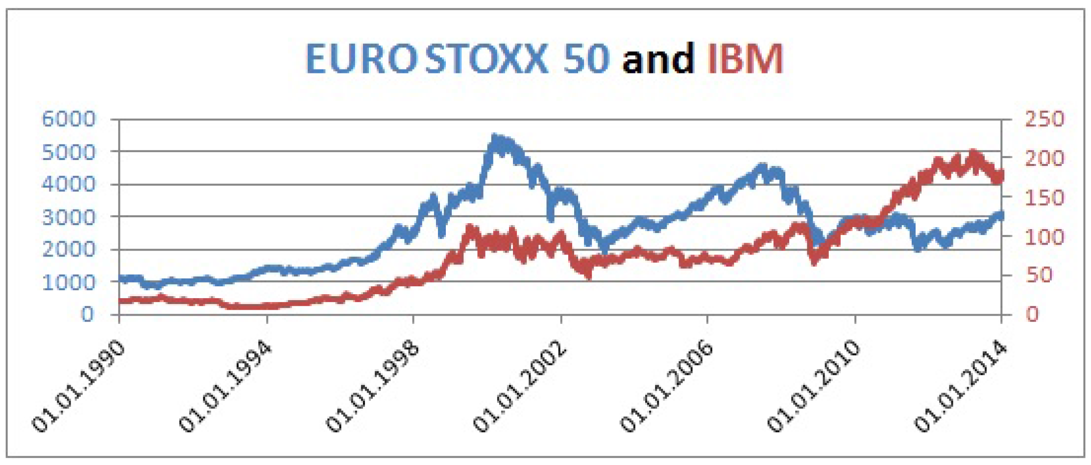
To derive empirical parameters from real stock market data, we created a dataset consisting of daily log returns of IBM (WKN: 851399 ISIN: US4592001014) and EURO STOXX50 (WKN 965814 ISIN EU0009658145) over the period from 1 January 1990 to 31 December 2013 (Figure 1). We take log returns into account, which are available for both time series. For the mentioned period of 24 years this approach results in 5998 log returns. The log returns are computed from the daily adjusted close prices (adjusted close prices are the stock or indices prices adjusted for all applicable splits and dividend distributions), which can be found at http://finance.yahoo.com/. As suggested by [29], we annualize the daily volatility by multiplying by the square root of 250 , which is the number of trading days instead of the number of calendar days.
Summary statistics:
| Log Returns | ||||
| EURO STOXX 50 | 4.33% | 21.84% | 0.3071 | |
| IBM | 10.22% | 28.81% |
In the next step, we compute the needed parameters for the explicit model (6), as well as for the implicit model (2). Hence, we use a moving window approach to compute the parameters and λ based on different non-overlapping samples of a window size k. Always starting from 31 December 2013 and going backwards in time, this approach results in a sample of size . The computed parameters , and , for each window of size k are used to compute the empirical cumulative distribution function and to derive the maximum likelihood estimates for the theoretical distributions. While the procedure for determining the correlation for both time series is straight forward, the common driver of randomness in volatility and eigenvalues needs some more investigations. After computing the parameters , , and for each of the time series separately, the samples (, and ) for the common randomness drivers are derived by:
In the explicit case, random volatility is modelled by , where the constant is already derived as 21.84% for EURO STOXX 50 and 28.81% for IBM. For the random driver in volatility, as well as for the random driver in eigenvalues, we divide the samples by their mean, ensuring that the parameters c and vary around one.
Measures of Goodness
Next, we evaluate the goodness of approximation of each of the suggested distributions in Section 1.1 by performing a test on the distributions of their variances, eigenvalues and correlations. By reviewing the literature for different measures of goodness of fit, it turns out that the number of statistical hypothesis tests for testing non-normal distributions is very limited (whereas there is a wide variety for testing normality). Nevertheless, the Kolmogorov–Smirnov (KS) test appears to be the standard nonparametric method as a goodness of fit test. To provide more substantiated results, we also take the Cramér–von Mises criterion as an alternative to the KS test into account ( Kuiper’s test and the Anderson–Darling test are also reasonable alternatives to the selected test, but these tests are only available for certain distributions):
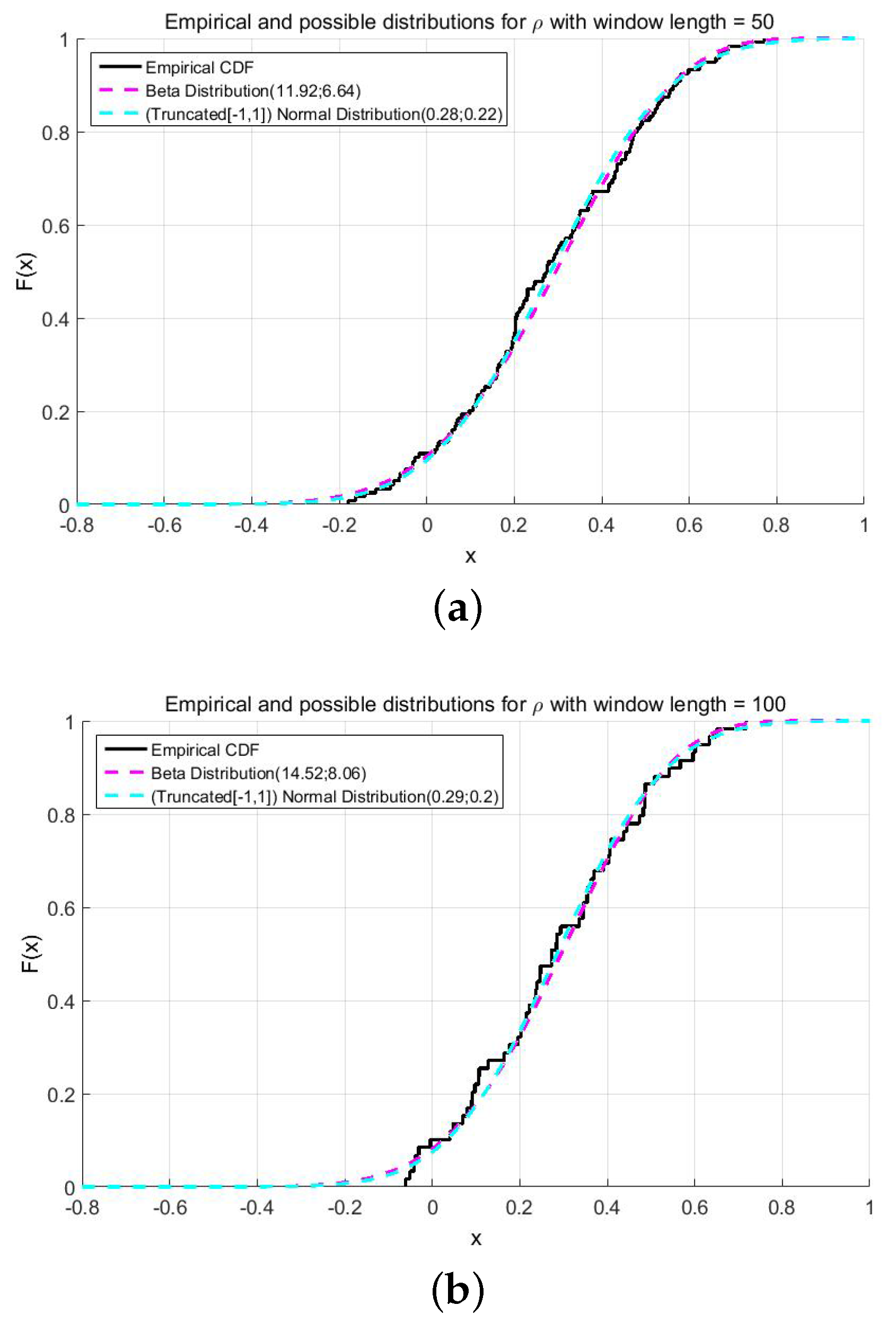
where is the empirical and the theoretical cumulative distribution function. While the Kolmogorov–Smirnov test is just based on the biggest distance between the empirical and the theoretical cumulative distribution function, the Cramér–von Mises criterion considers all of the deviations of the empirical distributionfrom the theoretical cumulative distribution function. After introducing two different measures of goodness, we study the different empirical cumulative distribution functions of c, ρ, and . We choose two different moving window sizes: and ; we obtain the resulting distribution, compute the maximum likelihood estimates (MLE) and provide the results from the statistical tests.
As one can infer from Figure 2 and Table 1, the obtained p-values from both test statistics (Equations (8) and (9)) hint that the transformed beta distribution and the truncated normal distribution are good choices to approximate the empirical distribution of ρ.
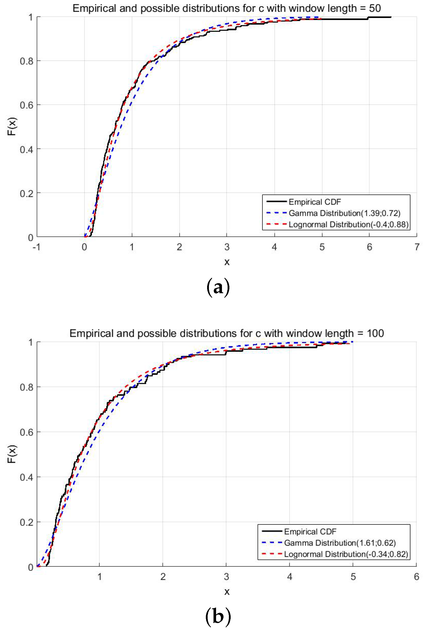
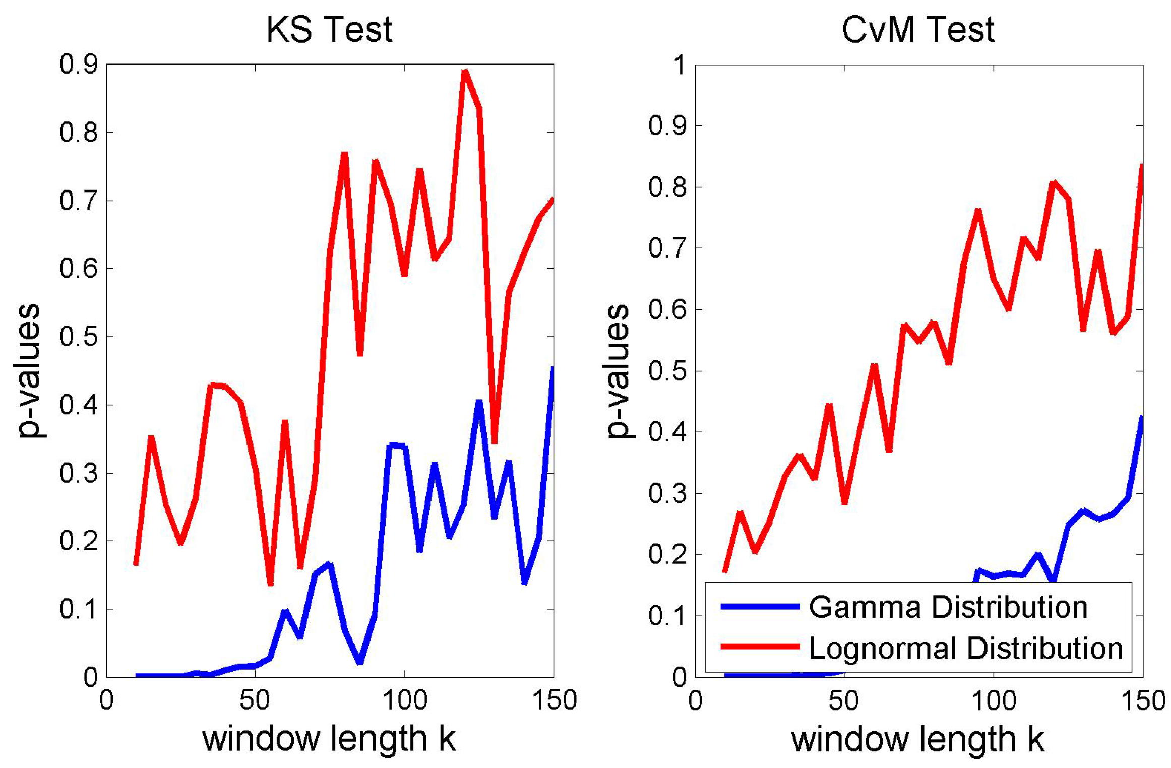
The p-values of Table 2, as well as Figure 3 show that the lognormal distribution approximates the empirical distribution of c. The small p-values from both hypothesis tests give evidence that the gamma distribution can be rejected as a suitable distribution of the empirical volatility driver.
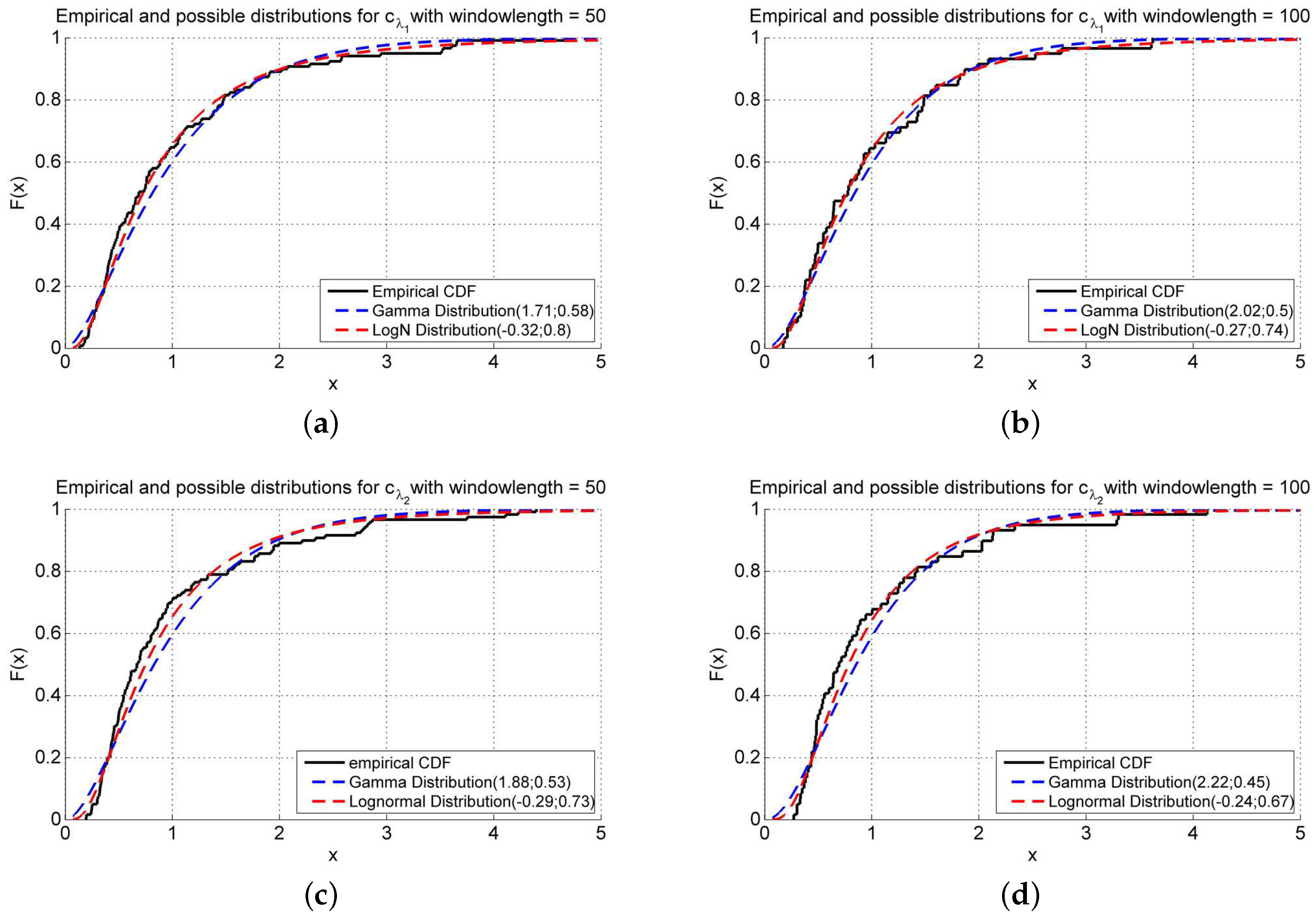
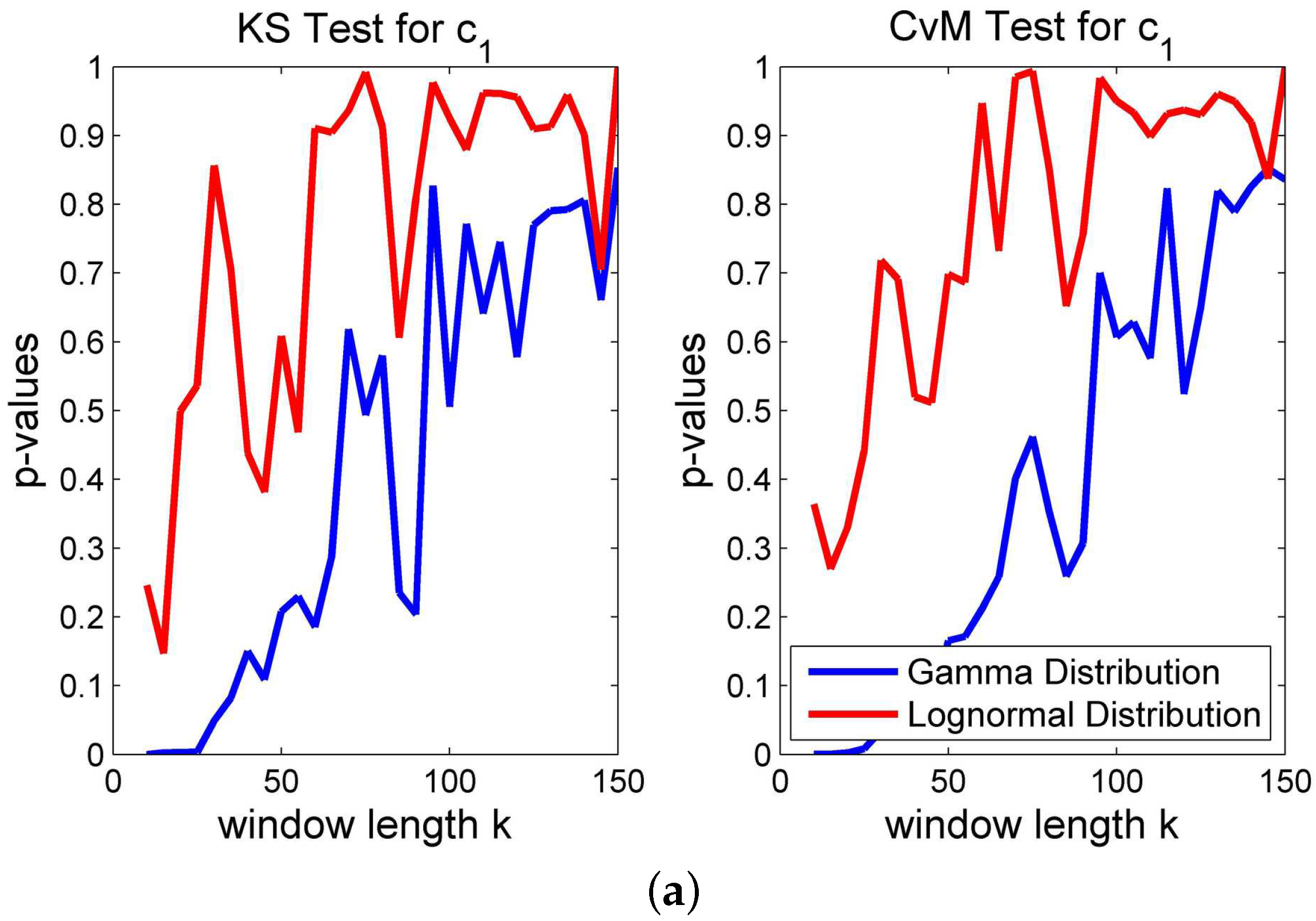
Figure 4 and Table 3 illustrate that the distribution of the first eigenvalue can be better approximated than the empirical distribution of the second eigenvalue. Furthermore, the lognormal distribution performs consistently better than the gamma distribution. This observation holds under both measures of goodness, for both moving window sizes and for both eigenvalues. In some cases (KS test and CvM-test for a moving window size of ), the gamma distribution can even be rejected.
After studying the distribution for exemplary moving window sizes and , we present the test results for moving window sizes for to obtain more general and consistent results. Afterwards, we summarize the main findings.
While higher p-values in Figure 5, Figure 6 and Figure 7 just support the assumption that the theoretical distribution matches the empirical one, small p-values of one of the tests provide very strong evidence against this assumption (the null hypothesis). The following can be inferred from Figure 5, Figure 6 and Figure 7:
• The truncated normal distribution, as well as the transformed beta distributions are good choices to approximate the empirical distribution with an acceptable degree of deviation, except for very small and unreliable moving window sizes. The works of [12,13] confirm that the (truncated) normal distribution is a good choice.
• In our setting, the lognormal distribution approximates the empirical distribution of consistently better than does the gamma distribution. This finding is consistent with [12,13], who found that the distribution of logarithmic standard deviations of daily returns is close to Gaussian.
• As one can infer from Figure 7, the approximations of the empirical distributions of the volatility driver of the two eigenvalues differ in a reasonable manner. The volatility of the first eigenvalue can be better approximated with the proposed theoretical distribution than can the volatility of the second. Nevertheless, under both measures of fit, the lognormal distribution approximates the empirical distribution of and consistently better than does the gamma distribution.
3.2. Pricing Derivatives with Empirical Parameters
Here, we use standard numerical integral functions of MATLAB (besseli to compute and trapz for double integrals) to generalize the constant covariance case in [1] to the random frameworks. We used a discretization of , integration limits of and limits of the infinite sum of 27, which ensure sufficient accuracy. The parameters from Table 2 and Table 3 are used to analyse the actual effect of random covariance. Therefore, we investigate the effects of the modelled random parameters , and on the prices of the mentioned double-digital option, its sub-product and on the correlation option with its less dimensional sub-product. This is done within our toy scenario of moving window sizes of and . For this toy scenario, we assume that and follow a lognormal distribution, while follows a truncated normal distribution. The parameters of these distributions can be inferred from Table 2 and Table 3.
As one can infer from Table 4, the difference in prices between the constant covariance and the random covariance could be very large. While the prices of with random covariance are at least 11% higher than the constant covariance prices, the prices of the correlation option are at most 11% lower by taking the random covariance into account. Therefore, random covariance could either lead to higher or to lower option prices, depending on the product at hand. In other words, failing to take into account estimation risk can lead to situations where the sell side underestimates the price of product by 26% or the investor of is charged 11% more. By comparing the explicit model with the implicit model, it can be observed that the explicit model consistently leads to higher price deviations from the constant covariance framework than the implicit model. Table 4 also highlights the differences between the double-barrier products and the single-barrier products. Both products and are more sensitive to the random covariance than the less dimensional barrier products and . Just by adding another barrier constraint, the impact of random covariance can be up to 6.9 percentage points higher ( explicit model, ). In other words, the impact of uncertainty increases when we deal with double-barrier products.
3.3. Analysis of Derivatives with Theoretical Parameters
In the final step, we move from the empirical parameters and distributions to theoretical scenarios and analyse further effects of the modelled random variables, as well as the impact of the sample size to highlight the price differences caused by parameter uncertainty (estimation errors). For reasons of simplicity, we slightly change the following parameters:
To investigate the separate effects of varying distributions of , and , we assume that follows a transformed beta distribution, while and follow again a lognormal distribution.
We start by analysing the explicit effect of varying the distribution parameters of correlation and volatility , followed by an analysis of the implicit effect on the covariance through random eigenvalues, where we distinguish between modelling just one eigenvalue and all eigenvalues.
3.3.1. Explicit Model
First, we investigate the separate effects of increasing uncertainty about rho:
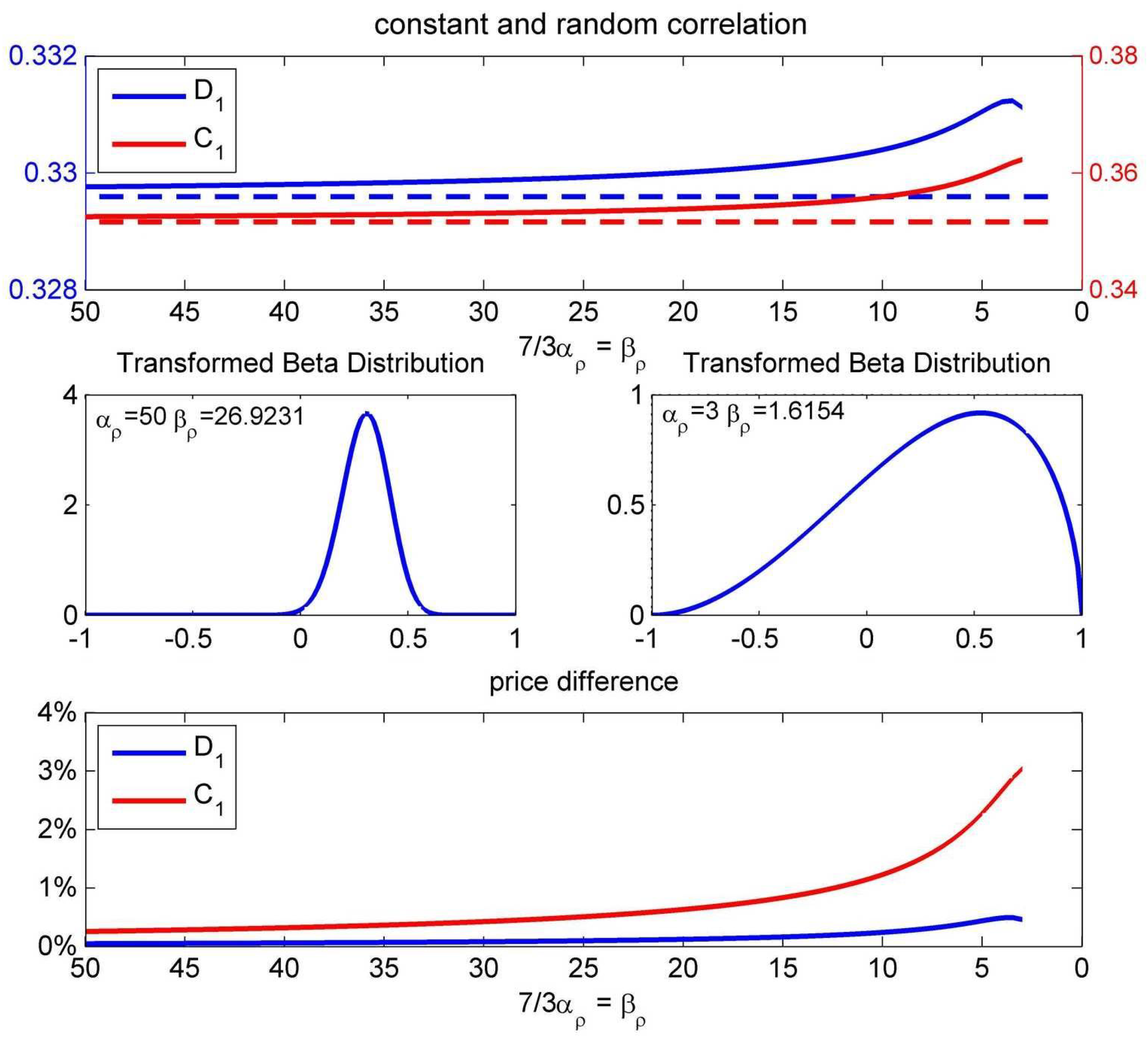
To measure theoretical price impacts resulting from uncertainty about correlation, we assume that follows a transformed beta distribution. We force the transformed beta distribution to vary around the mean of . As one can observe from Figure 8, with decreasing variation of the beta distribution, the prices of , as well as with random correlation converge to the price obtained with constant covariances. The increasing uncertainty about the correlation leads to slightly higher product prices of and .
While a very high uncertainty about the correlation leads to an increase of 3% in the product price of , the impact (about 0.5%) on the double-digital is even smaller. One of the reasons for the increase in prices is that higher correlation coefficients lead to higher probabilities of getting a payoff, whereas lower correlations lead to lower prices because the probability of crossing one of the barriers increases. Nevertheless, the impact of randomness in correlation is minimal although significant, because the correlation itself has a low impact on the prices of and . Next, we examine the separate effect of increasing uncertainty about volatility:
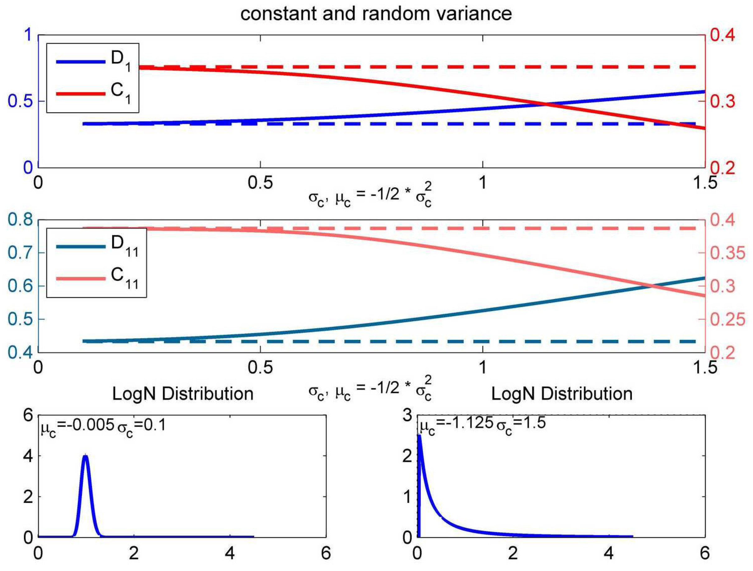
The impact of increasing uncertainty about volatility is quite significant for all of the considered products and . Again, we assume that follows a lognormal distribution with a forced mean to one. As already observed in the empirical section, the considered randomness leads to an increase in the double-digital options and to a decrease of the prices of the correlation options. Therefore, the seller of double-digital options should be aware of the fact that whenever he or she does not know volatility with a reasonable certainty, he or she might sell his or her option with a higher premium. Analogously, the investor in a correlation option should consider that he or she might claim a lower option price if there is a high degree of uncertainty about volatility.
In the case of the double-digital option , lower volatility leads to higher product prices, because the probability of expiring in the money increases, as well as not crossing any barrier. The effect of decreasing volatility for is ambiguous. On the one hand, the probability that one of the barriers will be crossed decreases, and this raises the price. However, on the other hand, the vanilla call options suffer from decreasing volatility (positive vega), because the probability of ending up in the money decreases. Due to the fact that the payoff structure of correlation options includes the product of two vanilla call options, here decreasing volatility leads to decreasing product prices. As one can infer from Figure 9, the considered lognormal distribution with and attaches much weight to prices obtained with low volatility; therefore, the random price of is lower than the constant price.
By separating the uncertainty about rho and volatility, as shown in Figure 8 and Figure 9, we can observe that the main driver for the price difference in Table 4 is the randomness in volatility. Increasing uncertainty about volatility can lead to a 74% higher product price of and to a 26% lower product price of . In the analysis of increasing uncertainty about volatility, we also consider the sub-products. Due to the fact that the sub-products and consider just one barrier constraint, they are less sensitive to changes in volatility. Therefore, uncertainty about volatility can lead to a price difference of −26% for and 44% for . Due to the payoff structure, the difference between and can be around 30 percentage points, whereas the highest price differences of and is around two percentage points.
3.3.2. Implicit Model
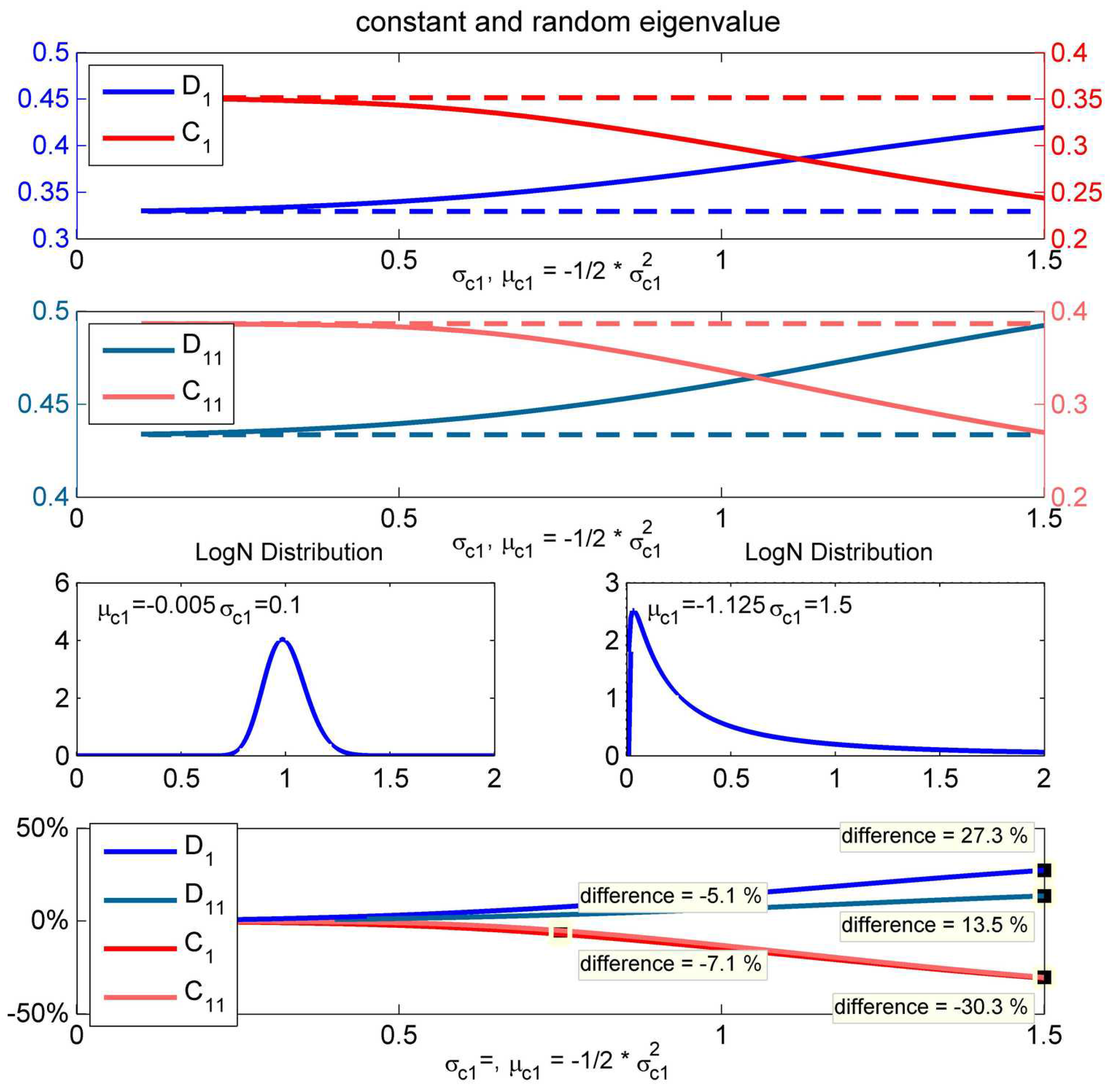
Next, we switch the explicit modelling to an implicit framework, which has the advantage that we are able to model the covariance with just one source of randomness in the respective eigenvalue. We start by analysing the effect of an increasing uncertainty about the first and largest eigenvalue .
As one can infer from the computed price differences in Figure 10, the modelled randomness in the largest eigenvalue of the covariance matrix leads to lower price differences than in Figure 9. Modelling only the first eigenvalue implies certainty about the second eigenvalue. This certainty is also reflected in the resulting volatilities. According to Model (2), our toy scenario results in the following matrix decomposition:
Therefore, we can compute the lowest possible values for volatility and correlation:
While modelling only the first eigenvalue to add randomness to the covariance, one can observe that is free to assume all possible values. Due to the fact that the lognormal distribution has a positive support, and always stay above their lowest possible value of 0.1716, respectively, 0.0568. Thus, restricting the number of modelled eigenvalues to one implies on the other hand that the practitioner is sure about the fact that and will not be lower than 0.1716 and 0.0568.
While the impact of these conditions leads to the highest possible price difference for of 27.3% and for of 13.5%, the impact on the correlation options and is very similar. Both prices of and can differ up to 30% compared to the constant price. As already observed, while the randomness has the same effect on the products and (around two percentage points), the effect on , can increase to a difference of 14 percentage points.
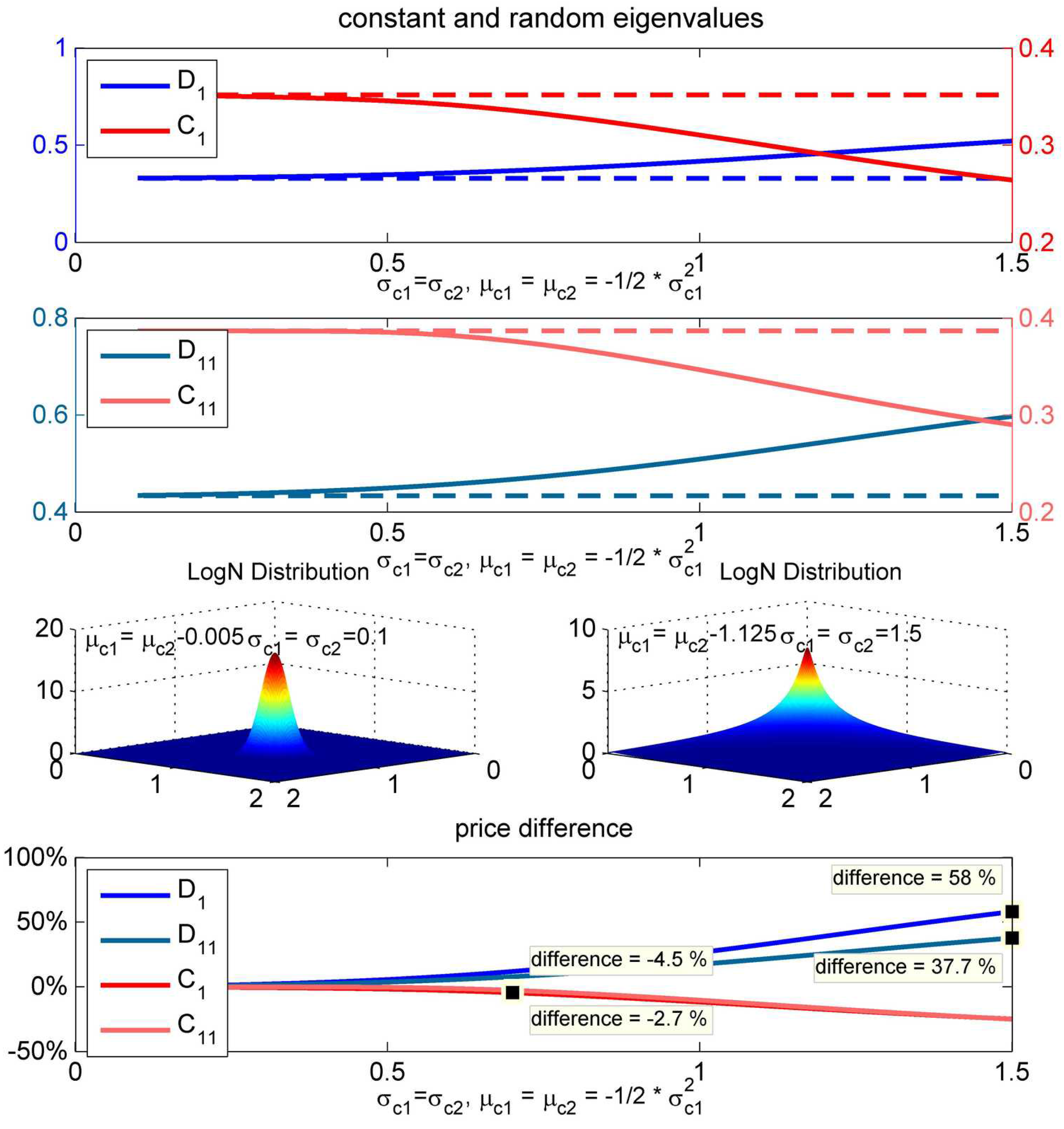
Alternatively to the previous analysis where we only modelled the first and largest eigenvalue, in the next analysis, we add randomness to both eigenvalues with a lognormal distribution (Figure 11).
Volatilities are now able to take all possible values, which results in more extreme scenarios, which on the other hand can lead to a price difference of 58% of , 38% of and −25% for and . While there are high price differences between and , the effect on and are at a comparable range.
To sum up, in the numerical section with theoretical parameters, the high differences between prices derived with constant and random covariance leads us to conclude that the distribution of point estimates should not be neglected. Furthermore, we detected that the additional consideration of a second barrier always magnifies the effect of random covariances.
4. Conclusions
This paper showed that closed-form formulas for pricing derivatives in a constant covariance framework from [1] can easily be generalized to introduce randomness in covariances. Therefore, we presented two different kinds of random covariance models, where the randomness in volatility and correlation is either explicitly or implicitly modelled. The introduced models are well suited to capture the discussed estimation risk, which originates from assuming the point estimate as the true value instead of considering theoretical or empirical distributions. In the numerical part of this paper, we derived empirical distributions of real data and highlighted the differences between the prices of well-known derivatives determined with constant and random covariances.
The price differences in some scenarios increased to 74% for a double-digital double-barrier option and could be in the range of for a double-barrier correlation option. The impact with regard to single-barrier options is lesser. Furthermore, we mainly point out two findings. First, randomness in volatility is the major driver for price differences. Second, derivatives with a larger number of barriers are more sensitive to random covariance and, therefore, have a higher estimation risk.
Author Contributions
The work was equally shared.
Conflicts of Interest
The authors declare no conflict of interest.
Appendix A. Proof of Theorem 1
The proof of this theorem is fully based on [1] with the simple addition of an iterative expectation.
The cited paper provides the solution to the inner expectation . Once this inner piece is known, then we integrated the covariance out numerically.
First, we find the inner expectation via risk-neutral valuation:
with:
By using the Feynman–Kac theorem, the Kolmogorov backward equation is obtained:
with conditions:
Next, we perform the following transformations:
with . This leads to:
with:
Next, the first order derivatives are removed by setting:
with:
The choice for α eliminates the first order derivatives with respect to the underlying while the choice of b eliminates the term Z:
with boundary and terminal conditions:
Using Feynman–Kac representation, the function Z can be written as:
with and
Next, we find the transition probability density function , which in the backward variables satisfies the following PDE:
with , and initial and boundary conditions:
This is the system of equations solved in [1], Theorem 2.2, page 222.
Recall the following relation between Z and q holds:
These are the steps in He et al.’s (1998) proof:
First, the second order mixed term derivatives are eliminated using a Cholesky decomposition of the covariance matrix .
where h satisfies the heat equation.
Second, a transformation to polar coordinates on is performed.
and are found exactly as in [1], pages 223 to 224, leading to solutions:
where and is the fundamental solution of the first kind for the Bessel equation. Substituting the expressions for R, Θ into the heat equation leads to a general solution of the form:
where are constants.
Third, this general solution has to satisfy the initial value condition for . Integrating with respect to λ leads to:
We conclude that the price (inner integral) is:
References
- H. He, W.P. Keirstead, and J. Rebholz. “Double Lookbacks.” Math. Financ. 8 (1998): 201–228. [Google Scholar] [CrossRef]
- J.D. Fonseca, M. Grasselli, and C. Tebaldi. “Option pricing when correlations are stochastic: An analytical framework.” Rev. Deriv. Res. 10 (2007): 151–180. [Google Scholar] [CrossRef]
- M. Escobar, and P. Olivares. “Pricing of mountain range derivatives under a principal component stochastic volatility model.” Appl. Stoch. Models Bus. Ind. 29 (2013): 31–44. [Google Scholar] [CrossRef]
- M. Escobar, B. Götz, D. Neykova, and R. Zagst. “Pricing two-assets Barrier Options under stochastic 519 correlation via perturbation theory.” Int. J. Theor. Appl. Financ. 18 (2015): 1550018. [Google Scholar] [CrossRef]
- P.P. Boyle, and A.L. Ananthanarayanan. “The impact of variance estimation in option valuation models.” J. Financ. Econ. 5 (1977): 375–387. [Google Scholar] [CrossRef]
- S.H. Lence, and D.J. Hayes. “Parameter-based Decision Making under Estimation Risk: An Application to Futures Trading.” J. Financ. 49 (1994): 345–357. [Google Scholar] [CrossRef]
- E. Jacquier, and R. Jarrow. “Bayesian analysis of contingent claim model error.” J. Econom. 94 (2000): 145–180. [Google Scholar] [CrossRef]
- R. Popovic, and D. Goldsman. “On valuing and hedging European options when volatility is estimated directly.” Eur. J. Oper. Res. 218 (2012): 124–131. [Google Scholar] [CrossRef]
- M. Rubinstein, and E. Reiner. “Breaking down the barriers.” Risk 4 (1991): 28–35. [Google Scholar]
- M. Escobar, S. Ferrando, and X. Wen. “Three dimensional distribution of Brownian motion extrema.” Stochastics 85 (2013): 807–832. [Google Scholar] [CrossRef]
- M. Escobar, and J. Hernandez. “A Note on the Distribution of Multivariate Brownian Extrema.” Int. J. Stoch. Anal. 2014 (2014): 1–6. [Google Scholar] [CrossRef]
- T.G. Andersen, T. Bollerslev, F.X. Diebold, and H. Ebens. “The distribution of realized stock return volatility.” J. Financ. Econ. 61 (2001): 43–76. [Google Scholar] [CrossRef]
- K.R. French, G. Schwert, and R.F. Stambaugh. “Expected stock returns and volatility.” J. Financ. Econ. 19 (1987): 3–29. [Google Scholar] [CrossRef]
- G. Letac, and H. Massam. “All Invariant Moments of the Wishart Distribution.” Scand. J. Stat. 31 (2004): 295–318. [Google Scholar] [CrossRef]
- S.L. Heston. “A closed-form solution for options with stochastic volatility with applications to bond and currency options.” Rev. Financ. Stud. 6 (1993): 327–343. [Google Scholar] [CrossRef]
- T. Lepage, S. Lawi, P. Tupper, and D. Bryant. Modelling the Rate of Evolution Using the CIR Process. Working Paper; Montreal, QC, Canada: McGill University, 2006. [Google Scholar]
- B. Chen, L.A. Grzelak, and C.W. Oosterlee. “Calibration and Monte Carlo Pricing of the SABR-Hull-White Model for Long-Maturity Equity Derivatives.” J. Comput. Financ. 15 (2011): 79–113. [Google Scholar] [CrossRef]
- C. Van Emmerich. Modeling Correlation as a Stochastic Process. Wuppertal, Germany: University of Wuppertal, 2006, Volume 6. [Google Scholar]
- L. Teng, C. van Emmerich, M. Ehrhardt, and M. Günther. “A versatile approach for stochastic correlation using hyperbolic functions.” Int. J. Comput. Math. 93 (2015): 524–539. [Google Scholar] [CrossRef]
- M. Escobar, B. Götz, L. Seco, and R. Zagst. “Pricing of spread options on stochastically correlated underlyings.” J. Comput. Financ. 12 (2009): 31–61. [Google Scholar] [CrossRef]
- W.G. Cochran, and J. Wishart. “The distribution of quadratic forms in a normal system, with applications to the analysis of covariance.” Math. Proc. Camb. Philos. Soc. 30 (1934): 178–191. [Google Scholar] [CrossRef]
- R.A. Fisher. “Frequency distribution of the values of the correlation coefficient in samples from an indefinitely large population.” Biometrika 10 (1915): 507–521. [Google Scholar] [CrossRef]
- B. Götz, M. Escobar, and R. Zagst. “Closed-Form Pricing of Two-Asset Barrier Options with Stochastic Covariance.” Appl. Math. Financ. 21 (2014): 363–397. [Google Scholar] [CrossRef]
- G. Bakshi, and D. Madan. “Spanning and derivative-security valuation.” J. Financ. Econ. 55 (2000): 205–238. [Google Scholar] [CrossRef]
- M. Dempster, A. Howarth, and G.S. Hong. “Spread Options Valuation and the Fast Fourier Transform.” In Mathematical Finance—Bachelier Congress 2000. Berlin/Heidelberg, Germany: Springer, 2002. [Google Scholar]
- X. Burtschell, J. Gregory, and J.P. Laurent. “A Comparative Analysis of CDO Pricing Models under the Factor Copula Framework.” J. Deriv. 16 (2009): 9–37. [Google Scholar] [CrossRef]
- D.M. Pooley, P.A. Forsyth, K.R. Vetzal, and R.B. Simpson. “Unstructured meshing for two asset barrier options.” Appl. Math. Financ. 7 (2000): 33–60. [Google Scholar] [CrossRef]
- P.G. Zhang. Exotic Options: A Guide to Second Generation Options, 2nd ed. Singapore: World Scientific Publushing Co. Pte. Ltd., 2006. [Google Scholar]
- D.W. French. “The weekend effect on the distribution of stock prices.” J. Financ. Econ. 13 (1984): 547–559. [Google Scholar] [CrossRef]
- B.G. Manjunath, and S. Wilhelm. “Moments Calculation for the Double Truncated Multivariate Normal Density, 2009.” Available online: https://arxiv.org/abs/1206.5387 (accessed on 23 June 2012).
Figure 1.
Historical series of EURO STOXX50 (primary axis) and IBM (secondary axis).

Figure 2.
Possible and empirical distributions of ρ. (a) ; (b) .

Figure 3.
Possible and empirical distributions of c. (a) ; (b) .

Figure 4.
Possible and empirical distributions of and . (a) ; (b) ; (c) ; (d) .

Figure 5.
Different measures of fit for correlation.
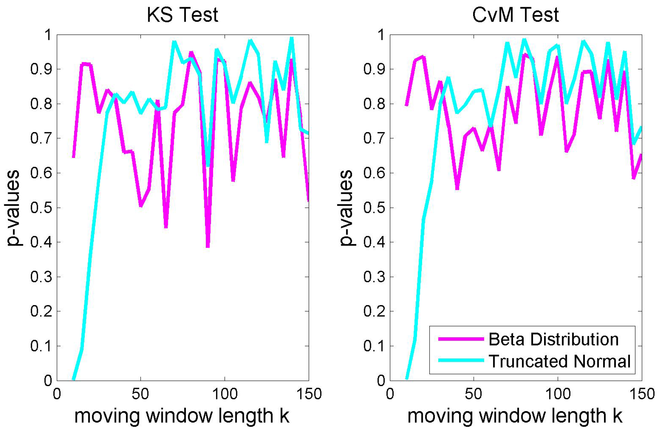
Figure 6.
Different measures of fit for volatility.

Figure 7.
Different measures of fit for eigenvalues resp. . (a) ; (b) .


Figure 8.
Effect of increasing uncertainty about and price differences between random and constant correlation.
Figure 8.
Effect of increasing uncertainty about and price differences between random and constant correlation.

Figure 9.
Effect of increasing uncertainty about and price differences between random and constant volatility.
Figure 9.
Effect of increasing uncertainty about and price differences between random and constant volatility.

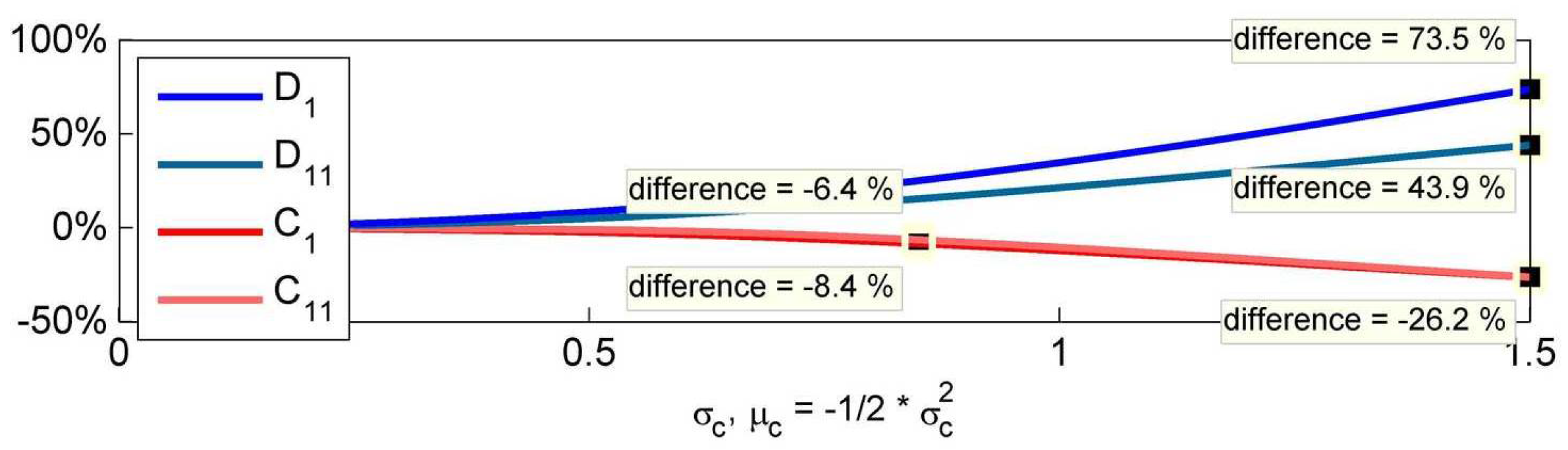
Figure 10.
Effect of increasing uncertainty about one eigenvalue () and price differences between random and constant covariance.
Figure 10.
Effect of increasing uncertainty about one eigenvalue () and price differences between random and constant covariance.

Figure 11.
Effect of increasing uncertainty about both eigenvalues () and price differences between random and constant covariance.
Figure 11.
Effect of increasing uncertainty about both eigenvalues () and price differences between random and constant covariance.


| ρ | p-Values | MLE | ||||||||
|---|---|---|---|---|---|---|---|---|---|---|
| KS-Test | CvM-Test | |||||||||
| Beta Dist. | 0.502 | 0.924 | 0.730 | 0.937 | 11.92 | 14.52 | 6.64 | 8.06 | ||
| Normal Dist. | 0.771 | 0.912 | 0.835 | 0.970 | 0.28 | 0.29 | 0.22 | 0.20 | ||
The parameters for the truncated normal distribution for ρ are estimated from the non-truncated distribution. The correct and more complex approach (see [30]) is negligible because the probability of values outside the interval is very small and the impact of the truncation is very small.
| c | p-Values | MLE | ||||||||
|---|---|---|---|---|---|---|---|---|---|---|
| KS-Test | CvM-Test | |||||||||
| Gamma Dist. | 0.015 | 0.339 | 0.011 | 0.164 | 1.39 | 1.61 | 0.72 | 0.62 | ||
| Lognormal Dist. | 0.304 | 0.589 | 0.282 | 0.649 | −0.4 | −0.34 | 0.88 | 0.82 | ||
| p-Values | MLE | ||||||||||
|---|---|---|---|---|---|---|---|---|---|---|---|
| KS-Test | CvM-Test | ||||||||||
| Gamma Dist. | 0.208 | 0.505 | 0.165 | 0.607 | 1.71 | 2.02 | 0.58 | 0.50 | |||
| Lognormal Dist. | 0.608 | 0.925 | 0.698 | 0.950 | −0.32 | −0.27 | 0.80 | 0.74 | |||
| Gamma Dist. | 0.046 | 0.320 | 0.022 | 0.157 | 1.88 | 2.22 | 0.53 | 0.45 | |||
| Lognormal Dist. | 0.319 | 0.545 | 0.239 | 0.458 | −0.29 | −0.24 | 0.73 | 0.67 | |||
| Constant | Random | ||||||||
|---|---|---|---|---|---|---|---|---|---|
| Covariance | Explicit Model (6) | Implicit Model(2) | |||||||
| Price | Rel.Diff | Price | Rel. Diff | ||||||
| Price | |||||||||
| 0.3331 | 0.4192 | 0.4062 | 25.8% | 21.9% | 0.3777 | 0.3693 | 13.4% | 10.9% | |
| 0.4284 | 0.5098 | 0.4957 | 18.9% | 15.6% | 0.4676 | 0.4604 | 9.1% | 7.4% | |
| 0.3639 | 0.3235 | 0.3299 | −11.1% | −9.3% | 0.3415 | 0.3476 | −6.1% | −4.5% | |
| 0.3952 | 0.3587 | 0.3661 | −9.2% | −7.4% | 0.3783 | 0.3854 | −4.3% | −2.5% | |
© 2016 by the authors; licensee MDPI, Basel, Switzerland. This article is an open access article distributed under the terms and conditions of the Creative Commons Attribution (CC-BY) license (http://creativecommons.org/licenses/by/4.0/).
Share and Cite
MDPI and ACS Style
Escobar, M.; Panz, S. A Note on the Impact of Parameter Uncertainty on Barrier Derivatives. Risks 2016, 4, 35. https://doi.org/10.3390/risks4040035
AMA Style
Escobar M, Panz S. A Note on the Impact of Parameter Uncertainty on Barrier Derivatives. Risks. 2016; 4(4):35. https://doi.org/10.3390/risks4040035
Chicago/Turabian StyleEscobar, Marcos, and Sven Panz. 2016. "A Note on the Impact of Parameter Uncertainty on Barrier Derivatives" Risks 4, no. 4: 35. https://doi.org/10.3390/risks4040035
Note that from the first issue of 2016, this journal uses article numbers instead of page numbers. See further details here.