Optimal Premium as a Function of the Deductible: Customer Analysis and Portfolio Characteristics

Abstract

An insurance company offers an insurance contract $(p,K)$, consisting of a premium p and a deductible K. In this paper, we consider the problem of choosing the premium optimally as a function of the deductible. The insurance company is facing a market of N customers, each characterized by their personal claim frequency, α, and risk aversion, β. When a customer is offered an insurance contract, she/he will, based on these characteristics, choose whether or not to insure. The decision process of the customer is analyzed in detail. Since the customer characteristics are unknown to the company, it models them as i.i.d. random variables; $A_1,\dots ,A_N$ for the claim frequencies and $B_1,\dots ,B_N$ for the risk aversions. Depending on the distributions of $A_i$ and $B_i$, expressions for the portfolio size $n(p;K)\in [0,N]$ and average claim frequency $\alpha (p;K)$ in the portfolio are obtained. Knowing these, the company can choose the premium optimally, mainly by minimizing the ruin probability.

1. Introduction

An insurance company has several instruments for stochastic control at its disposal. Much studied are dividends, reinsurance and investment; see, e.g., [1]. The present paper concentrates on premiums and deductibles. These are also obvious instruments, but have been somewhat less studied in the literature as such.

The standard model for the risk reserve $R_t$ at time t is the Cramer–Lundberg process:

$$R_t=r_0+ct-A_t,$$

where $r_0$ is the initial reserve, c is the gross premium rate and ${\left(A_t\right)}_{t\ge 0}$ is a compound Poisson process with parameters λ and F. More explicitly, $A_t={\sum }_{i=1}^{N_t}{Z}_i$ where ${\left(N_t\right)}_{t\ge 0}$ is a Poisson process with parameter λ counting the number of claims until time t, and the $Z_i$’s represent the (positive) claim sizes assumed to be i.i.d. and independent of ${\left(N_t\right)}_{t\ge 0}$, with common distribution F on $(0,\infty )$. Let $\overline{z}=\mathbb{E}\left[Z_i\right]$ and $\overline{z^2}=\mathbb{E}\left[Z_i^2\right]$. The Cramer–Lundberg process can, due to the arguments in [2], be approximated by the diffusion process:

$$\mathrm{d}{x}_t=\mu \mathrm{d}t+\sigma \mathrm{d}{W}_t,x_0=r_0$$

(1)

with $\mu =c-\lambda \overline{z}$ and ${\sigma }^2=\lambda \overline{z^2}$. To put it briefly, this diffusion process is the Brownian motion with drift that matches the mean and variance of the Cramer–Lundberg process at any given point in time.

We will describe an insurance contract by a premium p and a deductible K. The purpose, besides loss prevention and retention, of adding a deductible to a contract is to avoid administrating the numerous number of small claims. The deductible is therefore chosen to serve this purpose, and the premium will then be considered as a function of the chosen deductible. We will consider the methods of how to find the premium optimally in a given market. For simplicity, we assume that all (potential) customers are offered the same insurance contract $(p,K)$. We will also neglect the market effects by assuming that only one company supplies insurance.

A possible extension is to allow the insurance company to offer different deductibles and let the premium in the contract be regulated accordingly. A simple way of doing so is to say that the entire market can be divided into disjoint sub-markets, for example; one where there is a customer demand for a low deductible $K_l$, one for a medium deductible $K_m$ and one for a high deductible $K_h$. Therefore, the offered values of the deductibles will be $\{K_l,K_m,K_h\}$, where there is a separate market for each. It will then be possible to apply the same approach as considered here to each of the sub-markets.

There are several types of deductibles. We will consider the classical fixed amount deductible where the claims are truncated, so the loss for the insurance company in relation to a claim $Z_i$ can be described by the random variable:

$$\begin{array}{c}\hfill X_i^{\left(K\right)}={(Z_i-K)}^{+}=\left\{\begin{array}{cc}0,\hfill & \mathrm{if}{Z}_i<K,\hfill \\ Z_i-K,\hfill & \mathrm{if}{Z}_i\ge K.\hfill \end{array}\right.\end{array}$$

The risk reserve must therefore be modified:

$$R_t=r_0+ct-A_t^{\left(K\right)},$$

where $A_t^{\left(K\right)}$ is the compound Poisson process with losses $X_i^{\left(K\right)}$. Let $\overline{x^{n,\left(K\right)}}$ denote the n’th moment of $X_i^{\left(K\right)}$. Notice that $\overline{z}=\overline{x^{\left(0\right)}}$ and $\overline{z^2}=\overline{x^{2,\left(0\right)}}$, since the claims are assumed to be positive. The results here thus contain the no-deductible case.

Assume that the insurance company is facing a market consisting of N potential customers. Let $n(p;K)\in [0,N]$ denote the number of customers the insurance company attracts on the market when offering the contract $(p,K)$. Obviously, increasing the premium should lead to a loss of customers; therefore, it must be that $\frac{\partial n(p;K)}{\partial p}\le 0$. Furthermore, the average customer claim frequency in the portfolio will be denoted as $\alpha (p;K)$. Raising the premium will make it less attractive to insure for customers having low claim frequencies, and so, the average claim frequency of the portfolio increases, i.e., $\frac{\partial \alpha (p;K)}{\partial p}\ge 0$. This is commonly known as adverse selection. The gross premium c and the aggregate claim frequency λ will then depend on the premium, p, and the chosen deductible, K, as follows:

$$c(p;K)=n(p;K)p\mathrm{and}\lambda (p;K)=n(p;K)\alpha (p;K).$$

The drift and variance of the diffusion process (1) are modified accordingly:

$$\begin{array}{cc}\hfill \mu (p;K)& =n(p;K)p-\lambda (p;K)\overline{x^{\left(K\right)}}-L=n(p;K)\left(p-\alpha (p;K)\overline{x^{\left(K\right)}}\right)-L,\hfill \\ \hfill {\sigma }^2(p;K)& =\lambda (p;K)\overline{x^{2,\left(K\right)}}=n(p;K)\alpha (p;K)\overline{x^{2,\left(K\right)}}.\hfill \end{array}$$

In order to avoid trivialities, when minimizing the ruin probability at a later stage, a fixed liability payment rate L is introduced in the drift. Otherwise, the insurance company can choose p to be infinitely large such that no customer will insure, and the reserve will remain constantly at $r_0$, yielding a ruin probability of zero. The term liability is used in a broad sense. It covers any type of costs the insurance company might have. Let $\phi \left(r_0\right)$ denote the ruin probability as a function of the initial reserve when the reserve is modeled by the diffusion process. For more background on ruin theory, we refer to [3]. In this reference, it is also stated that when the drift $\mu (p;K)$ in the diffusion approximation is positive, then $\phi \left(r_0\right)=exp(-r_0\mu (p;K)/{\sigma }^2(p;K))$, and when the drift is negative, then ruin will be certain, i.e., $\phi \left(r_0\right)=1$ for any initial reserve $r_0$.

For a given deductible, changing the premium will have a double-sided effect on the drift (and profit) of the insurance company. Raising the premium will increase the earnings per customer, but will also reduce the size of the portfolio and increase the average claim rate due to adverse selection, and vice versa for decreasing the premium. In order to say which effect is dominating, a specification of the portfolio characteristics is needed.

First of all, we need to gain insight into the decision process of a customer. In this context, we introduce a risk aversion parameter β and motivate a method for incorporating risk aversion. See [4] for a microeconomic perspective of insurance.

In a naive setting, the customers would have the same claim rate, implying the average claim frequency to be constant, $\alpha (p;K)=\alpha$, and $n(p;K)$ could be chosen on some ad hoc form. In a more realistic setting, a market of potential customers is non-homogeneous in the sense that they have different characteristics, namely different α’s and β’s. A customer knows her/his own claim rate, but the insurer does not possess this information about the customers. The claim rates are therefore modeled as i.i.d. random variables $A_1,\dots ,A_N$ over the portfolio. Likewise for the risk aversion parameter, which will be considered as the outcomes of the i.i.d. random variables $B_1,\dots ,B_N$. This results in some less ad hoc forms for the functions $\alpha (p;K)$ and $n(p;K)$ to characterize the portfolio. Once the portfolio characteristics are known, the insurance company can use these to choose the premium optimally. The main optimization problem considered is minimizing the ruin probability, but this only makes sense in case of a positive drift in the diffusion (1). In the case of a negative drift ruin is certain, so the premium will be chosen to maximize the time to ruin.

The ideas here are very similar to the ones considered in [5]. The present paper takes however a different approach to risk aversion and, as said, incorporates deductibles. The work in [6] also finds the price of insurance as a function of the deductible for different types of deductibles, though not exploiting the aspects of risk aversion. The work in [7] also controls the gross premium indirectly by controlling the safety loading. All in all, the contributions of this paper are three-fold; analyzing the customer’s behavior in Section 2, finding portfolio characteristics in Section 3 and choosing the optimal premium for the insurance company in Section 4. For examples and illustrations, see Section 5.

2. Customer’s Problem

A potential customer has to make a decision on whether to insure or not, given that she/he is offered an insurance contract $(p,K)$. If the customer chooses to insure, she/he must pay a premium p at constant rate, but the customer can then report claims and get the amount above the threshold K covered. More specifically, if the customer experience a loss $Z_i$, she/he will only report it to the insurance company if $Z_i\ge K$ in which case she/he has to pay K herself/himself; otherwise, if $Z_i<K$, there is no purpose of reporting it, and she/he will have to cover the entire loss $Z_i$. On the other hand, if the customer chooses not to insure, she/he no longer has to pay p continuously. She/he will instead have to cover all of the uninsured losses by herself/himself.

For the moment, risk aversion is ignored, and the decision is made solely by comparing the present values of the wealth generated by the two options. Later risk aversion will be incorporated by pricing the excess uncertainty when not insuring using the variance premium principle. Let $V_I$ denote the present value of insuring and $V_{NI}$ of not insuring.

The customer is assumed to have a subjective discount rate d and access to a risk-free asset with interest rate r in which all her/his wealth is assumed to be invested. Furthermore, it is assumed that $d>r$ to ensure finite asset valuation. The customer is characterized by initial wealth $w_0$ and claim frequency α. The customer is furthermore assumed to have infinite life length. Remark 1 comments on this assumption. The problem of the customer will then be identical every period, and the decision will therefore not change over time.

We start by finding the present value of not insuring. As said, if the customer chooses not to insure, she/he will have to cover every loss herself/himself. Therefore, her/his wealth will develop according to:

$$\mathrm{d}{w}_t=r{w}_t\mathrm{d}t-\mathrm{d}{A}_t^{\alpha },$$

(2)

where ${\left(A_t^{\alpha }\right)}_{t\ge 0}$ is a compound Poisson process with parameters α and F, representing the total loss until time t for the potential customer when not insuring. Hence, $A_t^{\alpha }={\sum }_{i=1}^{N_t^{\alpha }}{Z}_i$ where ${\left(N_t^{\alpha }\right)}_{t\ge 0}$ is a Poisson process with parameter α assumed to be independent of the $Z_i$’s. Let ${\left(T_i\right)}_{i\in \mathbb{N}}$ denote the arrival times of the Poisson process ${\left(N_t^{\alpha }\right)}_{t\ge 0}$. Notice that (2) is an Ornstein–Uhlenbeck process driven by a Levy process (namely, the compound Poisson process), and the solution is therefore explicitly known as:

$$w_t=exp\left(rt\right)\left(w_0-{\int }_0^{t}exp(-rs)\mathrm{d}{A}_s^{\alpha }\right)=exp\left(rt\right)\left(w_0-\sum _{i=1}^{N_t^{\alpha }}exp(-r{T}_i)Z_i\right).$$

The present value of the wealth when not insuring is evaluated as:

$$V_{NI}=\mathbb{E}\left[{\int }_0^{\infty }exp(-dt)\mathrm{d}{w}_t\right].$$

Calculations given in Appendix A show that this can be reduced to:

$$V_{NI}=\frac{r{w}_0}{d-r}-\frac{\overline{z}\alpha }{d-r}.$$

On the other hand, if the customer chooses to insure, she/he will have to pay a premium continuously and cover the parts of the claims below the deductible. Her/his wealth will then have the following dynamics,

$$\mathrm{d}{w}_t=(r{w}_t-p)\mathrm{d}t-\mathrm{d}{A}_t^{\alpha ,K},$$

(3)

where ${\left(A_t^{\alpha ,K}\right)}_{t\ge 0}$ is the compound Poisson process representing the total loss associated with claims until time t for the customer when insuring, that is:

$$A_t^{\alpha ,K}=\sum _{i=1}^{N_t^{\alpha }}min\{Z_i,K\}=\sum _{i=1}^{N_t^{\alpha }}\left(K{\mathrm{𝟙}}_{\{Z_i\ge K\}}+Z_i{\mathrm{𝟙}}_{\{Z_i<K\}}\right).$$

Once again, we are looking at an Ornstein–Uhlenbeck process driven by a Levy process. This can be solved in the same way as seen previously,

$$\begin{array}{cc}\hfill w_t& =exp\left(rt\right)\left(w_0-{\int }_0^{t}exp(-rs)p\mathrm{d}t-{\int }_0^{t}exp(-rs)\mathrm{d}{A}_s^{\alpha ,K}\right)\hfill \\ & =exp\left(rt\right)\left(w_0-\frac{p}{r}\right)+\frac{p}{r}-exp\left(rt\right)\sum _{i=1}^{N_t^{\alpha }}exp(-r{T}_i)(K{\mathrm{𝟙}}_{\{Z_i\ge K\}}+Z_i{\mathrm{𝟙}}_{\{Z_i<K\}}).\hfill \end{array}$$

The present value of the wealth when insuring will therefore be:

$$V_I=\mathbb{E}\left[{\int }_0^{\infty }exp(-dt)\mathrm{d}{w}_t\right]=\frac{r{w}_0-p}{d-r}-\frac{\alpha }{d-r}\mathbb{E}[K{\mathrm{𝟙}}_{\{Z_i\ge K\}}+Z_i{\mathrm{𝟙}}_{\{Z_i<K\}}].$$

Since the approach and calculations are very similar to the ones used when finding $V_{NI}$, the details are skipped. We can now state the following.

Corollary 1.

Disregarding risk aversion, the customer will insure if and only if $V_I\ge V_{NI}$, which is equivalent to:

$$p\le \alpha \mathbb{E}\left[(Z_i-K){\mathrm{𝟙}}_{\{Z_i\ge K\}}\right]=\alpha \mathbb{E}[X_i^{\left(K\right)}]=\alpha \overline{x^{\left(K\right)}}$$

Hence, a risk-neutral customer will insure if the net premium (taking deductibles into account) exceeds the premium. She/he has no incentive to pay a loading in order to avoid the risk.

Remark 1.

The customer is assumed to have an infinite life length. This is obviously not realistic, but it is convenient for the analysis and not uncommon in other areas of non-life insurance. For example, it the basis for the standard use of the stationary distribution in bonus-malus systems; see the discussion in [8].

It would be more realistic with a random life length τ. In this case, the discount factor $exp(-dt)$ has to be replaced by $\mathbb{P}(\tau >t)exp(-dt)$ in the above formulas for the present values, $V_{NI}$ and $V_I$. This will in general change the analytic expressions. Though note that in the case where τ is exponential with rate, say, ρ, the same expressions appears with d replaced by $d+\rho$. Due to the forgetfulness property of the exponential distribution, the customer is still facing an identical problem every period. This leads to obvious reinterpretations of the analysis of this section. ☐

In order for insurance to make sense, the customer must of course have some degree of risk aversion. We want to find which excess risk the customer is exposed to when not insuring and how to price this risk when risk aversion is essential.

The first step is to notice that $V_{NI}$ also could have been derived in a more intuitive way. Recall that all wealth is assumed to be invested in the risk-free asset. Therefore, wealth itself has the dynamics $\mathrm{d}{w}_t=r{w}_t\mathrm{d}t$ of a bank account. When accumulating interest, this has present value:

$${\int }_0^{\infty }exp(-dt)\mathrm{d}{w}_t={\int }_0^{\infty }exp(-(d-r)t)r{w}_{0}dt=\frac{r{w}_0}{d-r}.$$

(4)

When a non-insured customer has to pay a loss $Z_i$ at time $T_i$, she/he also loses a possible interest rate income. Therefore, the total loss of paying $Z_i$ at time $T_i$ can be calculated using the formula (4) with the discounted loss $exp(-r{T}_i)Z_i$ as $w_0$. Hence,

$$V_{NI}=\frac{r{w}_0}{d-r}-\frac{r}{d-r}\mathbb{E}\left[\sum _{i=1}^{\infty }exp(-r{T}_i)Z_i\right].$$

Note that due to Campbell–Mecke’s formula (see, e.g., [9] for further details), this is in fact equal to the expression for $V_{NI}$ found previously. Furthermore, we have the following alternative characterization of $V_I$,

$$V_I=\frac{r{w}_0-p}{d-r}-\frac{r}{d-r}\mathbb{E}\left[\sum _{i=1}^{\infty }exp(-r{T}_i)(K{\mathrm{𝟙}}_{\{Z_i\ge K\}}+Z_i{\mathrm{𝟙}}_{\{Z_i<K\}})\right]$$

which could have been explained with a similar intuitive approach using truncated losses.

The criteria of insuring in Corollary 1 when disregarding risk aversion can then be expressed as the inequality:

$$p\le \mathbb{E}\left[r\sum _{i=1}^{\infty }exp(-r{T}_i)(Z_i-K){\mathrm{𝟙}}_{\{Z_i\ge K\}}\right].$$

The additional risk the customer is exposed to when not insuring can therefore be captured by the random variable:

$$S^{\left(K\right)}=r\sum _{i=1}^{\infty }exp(-r{T}_i)(Z_i-K){\mathrm{𝟙}}_{\{Z_i\ge K\}}=r\sum _{i=1}^{\infty }exp(-r{T}_i)X_i^{\left(K\right)}.$$

The next step is to find the maximum premium the risk averse customer is willing to pay, also called her/his reservation price for this risk. Inspired by microeconomics, one can let the customer’s preferences be represented by a concave utility function $u\left(·\right)$. Assume that the only risk the customer is concerned about when pricing is the additional risk $S^{\left(K\right)}$ she/he is carrying when not insuring. The losses less than or equal to the deductible is a risk that the customer is also facing, but cannot be insured against; see Remark 3 for further details. Inspired by [10], the maximal premium $P\left(K\right)$ the customer is willing to pay for an insurance of a risk $S^{\left(K\right)}$ is the solution to the equation:

$$\mathbb{E}[u(w-S^{\left(K\right)})]=u(w-P\left(K\right)).$$

(5)

Therefore, the customer’s reservation price satisfies that she/he is indifferent between carrying the risk $S^{\left(K\right)}$ and paying the premium $P\left(K\right)$.

A possible choice is to let the customer’s preferences be represented by an exponential utility function,

$$u_{\gamma }\left(x\right)=\frac{1}{\gamma }(1-exp(-\gamma x)),$$

where γ is a risk aversion parameter. The premium in (5) can then be solved explicitly as:

$$P_{\exp }\left(K\right)=\frac{1}{\gamma }log(\mathbb{E}[exp(\gamma S^{\left(K\right)})]).$$

(6)

This is the same premium as found in [11], where it is the insurer, not the insured, pricing a risk. It is commonly known as the exponential premium principle and is mostly used by the insurer in the literature.

The object is to obtain an analytic expression for the premium, and this is extremely complicated (if not impossible without having to make a lot of simplifying assumptions) to get for $P_{\exp }\left(K\right)$. This is mainly due to $S^{\left(K\right)}$ being a sum of dependent random variables caused by the dependence structure in the $T_i$’s. Thus, the additivity property that [11] proves the exponential premium principle possesses cannot be used. To illustrate this complexity, a simple case example is presented in Appendix C. In order to obtain a more simple expression, a second order Taylor approximation of the logarithm in (6) around $\gamma =0$ is considered,

$$P_{\exp }\left(K\right)\approx \mathbb{E}[S^{\left(K\right)}]+\frac{\gamma }{2}\mathbb{V}\mathrm{ar}[S^{\left(K\right)}].$$

Assessments about the premium will be based on the right-hand side hereinafter. Let $\beta =\gamma /2$ and introduce the notation:

$$P_{\mathrm{var}}\left(K\right)=\mathbb{E}[S^{\left(K\right)}]+\beta \mathbb{V}\mathrm{ar}[S^{\left(K\right)}].$$

(7)

This the well-known variance premium principle. It expands the net premium principle by adding a risk loading that is proportional by a factor $\beta >0$ to the variance of the risk. Therefore, the customer is now further characterized by the risk aversion coefficient β. Approximating the exponential premium principle by the variance premium principle is a common approach; see, for example, [10].

It is indeed possible to find an analytic expression for (7). Applying Campbell–Mecke’s formula, it appears that the expectation term simply is:

$$\mathbb{E}[S^{\left(K\right)}]=\alpha \overline{x^{\left(K\right)}}.$$

The variance term in (7) is calculated using the total law of variance in Appendix B, giving the result:

$$\mathbb{V}\mathrm{ar}[S^{\left(K\right)}]=\frac{r\overline{x^{2,\left(K\right)}}\alpha }{2}.$$

The concluding premium is summarized below.

Corollary 2.

Given a deductible K, the customer is facing the excess risk $S^{\left(K\right)}=r{\sum }_{i=1}^{\infty }exp(-r{T}_i)X_i^{\left(K\right)}$ when not insuring and is willing to pay the following price for an insurance:

$$\begin{array}{c}\hfill P_{var}\left(K\right)=\alpha \overline{x^{\left(K\right)}}+\beta \left(\frac{r\overline{x^{2,\left(K\right)}}\alpha }{2}\right)=\left(1+\beta \frac{r\overline{x^{2,\left(K\right)}}}{2\overline{x^{\left(K\right)}}}\right)\alpha \overline{x^{\left(K\right)}}.\end{array}$$

(8)

In Example 1, the premium (8) is calculated explicitly for log-normally-distributed claim sizes.

Remark 2.

The approach leads to a fairly classical premium calculation principle, which in the literature is mostly seen from the insurer’s perspective. This motivates the use of other already developed premium calculation principles applied from the the customer’s point of view. An example of such is the standard deviation principle, where the premium depends on the mean and the standard deviation of the risk in a linear structure,

$$P_{\mathrm{std}}\left(K\right)=\mathbb{E}[S^{\left(K\right)}]+\beta \sqrt{\mathbb{V}\mathrm{ar}[S^{\left(K\right)}]}.$$

Since we already have expressions for the mean and the variance, we can write this more explicitly as:

$$P_{\mathrm{std}}\left(K\right)=\alpha \overline{x^{\left(K\right)}}+\beta \sqrt{\left(\frac{r\overline{x^{2,\left(K\right)}}\alpha }{2}\right)}.$$

Another could simply be the expected value premium principle with a safety loading depending on the individual’s risk aversion:

$$P_{\mathrm{ev}}\left(K\right)=(1+\omega \left(\beta \right))\mathbb{E}\left[S\right]=(1+\omega \left(\beta \right))\alpha \overline{x^{\left(K\right)}}.$$

(9)

The latter gives a simple expression, even though it still has a nice intuitive interpretation. All evaluations in the following will be based on the variance premium principle. However, do note that a similar approach can be used with other premium calculation principles.  ☐

Remark 3.

The risk the customer is facing can be split into two. First of these is the risk the customer cannot insure. This is the (part of the) losses that the customer must pay regardless of insuring or not and is the uncertainty that appears in both $V_n$ and $V_i$. The monetary value at Time 0 of this risk can be deduced to:

$$S^{\le K}=r\sum _{i=1}^{\infty }exp(-r{T}_i)(Z_i{\mathrm{𝟙}}_{\{Z_i<K\}}+K{\mathrm{𝟙}}_{\{Z_i\ge K\}}).$$

Second of these is the additional risk $S^{\left(K\right)}$ the customer can buy insurance to cover. The maximum premium that the customer is willing to pay in (5) will be altered as follows if she/he takes $S^{\le K}$ into consideration,

$$\mathbb{E}[u(w_0-S^{\le K}-S^{\left(K\right)})]=\mathbb{E}[u(w_0-S^{\le K}-P\left(K\right))].$$

Using the exponential utility and solving yields:

$$P\left(K\right)=\frac{1}{\gamma }log\left(\frac{\mathbb{E}[exp(\gamma S^{\le K}+\gamma S^{\left(K\right)})]}{\mathbb{E}[exp\left(\gamma S^{\le K}\right)]}\right).$$

Proceeding to a similar second order Taylor approximation as seen previously,

$$P_{exp}\left(K\right)\approx \mathbb{E}[S^{\left(K\right)}]+\frac{\gamma }{2}\mathbb{V}\mathrm{ar}[S^{\left(K\right)}]-\gamma \mathbb{C}\mathrm{ov}(S^{\le K},S^{\left(K\right)}),$$

it appears that in the final pricing formula, the assumption about the customer only caring about pricing the excess risk $S^{\left(K\right)}$ regardless of $S^{\le K}$ corresponds mathematically to assuming that $\mathbb{C}\mathrm{ov}(S^{\le K},S^{\left(K\right)})\approx 0$. A similar comment is also made in [10].  ☐

3. Portfolio Characteristics

A customer is characterized by her/his claim frequency α and risk aversion β. As previously commented, these characteristics are most likely customer-dependent. The insurance company therefore considers them as random variables being i.i.d. on the market. The claim frequencies are represented by $A_1,\dots ,A_N$, and the risk aversions by $B_1,\dots ,B_N$. First, we will consider the claim frequency as being random and the risk aversion as constant. Next, we will reverse it, by modeling the risk aversion as random and letting the claim frequency be constant. A third, more advanced, possibility is of course to let the customer characteristics $(\alpha ,\beta )$ be represented by random vectors $(A_1,B_1),\dots ,(A_N,B_N)$. This complicates the evaluations considerably and is therefore left open by this paper.

In each case, we derive an expression for the portfolio size and for the average claim frequency in the portfolio. These expressions will become explicit functions when assuming a concrete distribution.

3.1. Stochastic Claim Frequencies

Consider the first case mentioned above, where the risk aversion is constant, and the claim frequency of the customer is unknown to the insurance company and, therefore, modeled by a random variable denoted by A. As said, we want to find the expected size of the portfolio and the average claim rate in it.

From the reservation price in (8), it follows that a customer with characteristics $(\alpha ,\beta )$ will insure if the offered insurance contract $(p,K)$ satisfies the inequality:

$$p\le \alpha \overline{x^{\left(K\right)}}+\frac{\beta \alpha r}{2}\overline{x^{2,\left(K\right)}}.$$

Since the claim frequency is modeled by a random variable, A, to the insurer, this translates to the relation:

$$A\ge \frac{2p}{2\overline{x^{\left(K\right)}}+\beta r\overline{x^{2,\left(K\right)}}}.$$

The expected portfolio size will then be the probability of this event happening multiplied by the size of the market, namely:

$$n(p;K)=\mathbb{P}\left(A\ge \frac{2p}{2\overline{x^{\left(K\right)}}+\beta r\overline{x^{2,\left(K\right)}}}\right)N.$$

This is the mean demand curve as a function of the premium and deductible. In the following, it is assumed that N is large and that there is a continuum of customers, such that the deviation from the actual demand curve is negligible.

The average claim frequency rate in the portfolio is the expected claim frequency given that the customer chooses to insure, i.e.,

$$\alpha (p;K)=\mathbb{E}\left[A|A\ge \frac{2p}{2\overline{x^{\left(K\right)}}+\beta r\overline{x^{2,\left(K\right)}}}\right].$$

Exponentially-Distributed Claim Frequencies

When accounting for unobserved heterogeneity in the Bayesian claim experience rating setting, the claim frequency is frequently assumed to be $\Gamma (s,b)$ distributed, for example, as in [12]. In some cases there are empirical evidence of s being close to one. See [13] for more discussion. This motivates the assumption of an exponential distribution with parameter b of the claim frequency A. Offering the contract $(p,K)$, the customer will insure with probability:

$$\mathbb{P}\left(A\ge \frac{2p}{2\overline{x^{\left(K\right)}}+\beta r\overline{x^{2,\left(K\right)}}}\right)=exp\left(-b\frac{2p}{2\overline{x^{\left(K\right)}}+\beta r\overline{x^{2,\left(K\right)}}}\right).$$

This yields a portfolio size of:

$$n(p,K)=exp\left(-b\frac{2p}{2\overline{x^{\left(K\right)}}+\beta r\overline{x^{2,\left(K\right)}}}\right)N.$$

The exponential distribution has a memoryless property, which implies $\mathbb{E}\left[A\right|A\ge a]=1/b+a$. The expected claim frequency of an insured customer will therefore be :

$$\alpha (p,K)=\frac{2p}{2\overline{x^{\left(K\right)}}+\beta r\overline{x^{2,\left(K\right)}}}+\frac{1}{b}.$$

This equation reflects adverse selection very clearly, since $\alpha (p,K)$ is linearly increasing in p.

Remark 4.

If the customer’s reservation price was defined by the expected value premium principle (9), the portfolio characteristics would be:

$$n(p;K)=\mathbb{P}\left(A\le \frac{p}{(1+\omega \left(\beta \right))\overline{x^{\left(K\right)}}}\right)N,\alpha (p;K)=\mathbb{E}\left[A|A\le \frac{p}{(1+\omega \left(\beta \right))\overline{x^{\left(K\right)}}}\right].$$

Assuming an exponentially-distributed claim frequency, the characteristics become:

$$n(p;K)=exp\left(-b\frac{p}{(1+\omega \left(\beta \right))\overline{x^{\left(K\right)}}}\right)N,\alpha (p;K)=\frac{p}{(1+\omega \left(\beta \right))\overline{x^{\left(K\right)}}}+\frac{1}{b}.$$

This is slightly easier to work with and has the advantage that $\omega \left(\beta \right)$ can be chosen on a simple form.☐

3.2. Stochastic Risk Aversions

Instead of letting a customer being represented by a stochastic claim frequency and constant risk aversion, we now turn it around. Assume that the customer now has a constant claim frequency α. This is indeed relevant to consider. For example, everyone could be equally disposed to disaster caused by nature. Furthermore, assume that the risk aversion is represented by a random variable B. The criterion (8) of insuring for a given contract $(p,K)$ can then be stated as:

$$B\ge \frac{2p-2\alpha \overline{x^{\left(K\right)}}}{r\overline{x^{2,\left(K\right)}}\alpha }.$$

Therefore, the portfolio size will be characterized by:

$$n\left(p\right)=\mathbb{P}\left(B\ge \frac{2p-2\alpha \overline{x^{\left(K\right)}}}{r\overline{x^{2,\left(K\right)}}\alpha }\right)N.$$

Gamma Distributed Risk Aversions

Risk aversion is somewhat an abstract concept. It is therefore difficult to suggest a distribution since there is limited literature available. Since the Gammadistribution is a popular choice for the claim frequency, we choose to consider the same distribution for the risk aversion. Assuming that the risk aversion has an $\Gamma (w,\nu )$ distribution, the demand curve will have the form:

$$n\left(p\right)=\frac{\Gamma (w,\nu (2p-2\alpha \overline{x^{\left(K\right)}})/\left(r\overline{x^{2,\left(K\right)}}\alpha \right))}{\Gamma \left(w\right)}N.$$

In the case $w\approx 1$, the distribution approximately reduces to an exponential distribution with parameter ν, and the portfolio size will then simply be:

$$n\left(p\right)=exp\left(-\nu \frac{2p-2\alpha \overline{x^{\left(K\right)}}}{r\overline{x^{2,\left(K\right)}}\alpha }\right)N.$$

4. Ruin Probability

In this section, we consider the optimization problem of the insurance company. It mainly wants to minimize the ruin probability, but as this only makes sense for a positive drift, the expected time to ruin is considered in the case of a negative drift. The overall aim is to find the optimal premium as a function of the deductible.

When the controlled reserve develops according to a Brownian motion with positive drift, [14] shows that minimizing the ruin probability is equivalent to maximizing the following ratio $\mu /\sigma$ between the drift and volatility. In our setting, this means maximizing:

$$\frac{\mu (p;K)}{{\sigma }^2(p;K)}=\frac{p-\alpha (p;K)\overline{x^{\left(K\right)}}}{\alpha (p;K)\overline{x^{2,\left(K\right)}}}-\frac{L}{n(p;K)\alpha (p;K)\overline{x^{2,\left(K\right)}}}.$$

(10)

This also follows from the relation $\phi \left(r_0\right)=exp(-2r_0\mu (p;K)/{\sigma }^2(p;K))$. Recall that if the drift is negative, then $\phi \left(r_0\right)=1$.

As previously implied, if the market consists of risk-neutral customers, then the drift of the diffusion process will be negative, making ruin certain. In order to avoid this, it is assumed in the following that there is a sufficiently large degree of risk aversion among the (potential) customers to satisfy the net profit condition $p>\alpha (p;K)\overline{x^{\left(K\right)}}$ for some p. Otherwise, there will be no motivation for selling insurance.

Notice that if $p=0$, the insurance company will offer insurance for free, and so, $\mu (0;K)<0$ for any given K. Furthermore, due to the liability rate, L, the diffusion will also have a negative drift when the premium becomes very high, since no customer will then be interested in insuring, hence ${lim}_{p\to \infty }\mu (p;K)<0$. Thus, ruin will be certain for both $p=0$ and $p\to \infty$.

Now, assume for some K that the premium is zero. What will then happen if the premium was raised marginally? The insurance company will have nearly the same amount of customers and, therefore, also the same amount of claims, but the firm will get a small revenue when collecting premiums. Hence, $\mu (p,K)$ will increase. Note, that this is under the assumption that the effect from portfolio size decrease and adverse selection is smaller than the effect of raising the premium. Conversely, what if the premium was so high that no customer would be interested in insuring? Recall that there are N customers on the market and that each customer has a reservation price for insurance (depending on the customer characteristics). Therefore, if the insurance company sets the premium so high that it is above the reservation price of all N customers, then no customer will insure. Though if the company lowers the premium enough for it to become below the reservation price of the most risky/risk adverse potential customers on the market, then under the condition of $p>\alpha (p,K)\overline{x^{\left(K\right)}}$, the insurance company will obtain some revenue to cover at least some of the liability cost. Hence, $\mu (p,K)$ will also increase when lowering the premium for very large values. This tells us intuitively that if there is an optimal premium, then it is not obtained for $p=0$, nor in the limit $p\to \infty$, and we thereby avoid trivialities when finding the optimal premium.

Abbreviate notation by ${\mu }_p(p,K)=\frac{\partial \mu (p;K)}{\partial p}$ and similarly for ${\alpha }_p(p,K)$ and $n_p(p,K)$. Assume that there is a unique $\tilde{p}$ that maximizes the drift, i.e., satisfies the first order conditions:

$${\mu }_p(\tilde{p};K)=n_p(\tilde{p};K)\left(\tilde{p}-\alpha (\tilde{p};K)\overline{x^{\left(K\right)}}\right)+n(\tilde{p};K)\left(1-{\alpha }_p(\tilde{p};K)\overline{x^{\left(K\right)}}\right)=0.$$

(11)

This is equivalent to saying that $\tilde{p}$ must satisfy:

$$\frac{-n_p(\tilde{p};K)}{n(\tilde{p};K)}=\frac{1-{\alpha }_p(\tilde{p};K)\overline{x^{\left(K\right)}}}{\tilde{p}-\alpha (\tilde{p};K)\overline{x^{\left(K\right)}}}.$$

The intuitive interpretation is that the relative marginal change in the demand curve must equal the relative marginal change in average net revenue per customer due to a change in premium. Two cases then arise:

(i)

If $\mu (\tilde{p};K)>0$, then $\phi \left(r_0\right)<1$ for all $r_0>0$, $K>0$ and p in some bounded open interval $I\subset (0,\infty )$ containing $\tilde{p}$.

(ii)

If $\mu (\tilde{p};K)\le 0$, then $\phi \left(r_0\right)=1$ for all $r_0>0$ and $p>0$.

Notice that the drift is positive if the net profit per customer is greater than the liability cost per customer, that is $p-\alpha (p;K)>L/n(p;K)$. This is more strict than the net profit condition.

Since the current framework is very general, so will the results be. In every concrete application, the existence of a unique solution must be verified. In Case (i), an optimization criterion is given and proven in Theorem 1.

Theorem 1.

When $\mu (\tilde{p};K)>0$, the optimal premium minimizing the ruin probability must be a solution to the equation:

$$1-p\frac{{\alpha }_p(p;K)}{\alpha (p;K)}+\frac{L}{n(p;K)}\left(\frac{n_p(p;K)}{n(p;K)}+\frac{{\alpha }_p(p;K)}{\alpha (p;K)}\right)=0.$$

Proof. 

Differentiating (10) with respect to the premium,

$$\begin{array}{cc}\hfill \frac{\partial \left(\frac{\mu (p;K)}{{\sigma }^2(p;K)}\right)}{\partial p}=& \frac{1-{\alpha }_p(p;K)\overline{x^{\left(K\right)}}}{\alpha (p;K)\overline{x^{2,\left(K\right)}}}-\frac{\left(p-\alpha (p;K)\overline{x^{\left(K\right)}}\right){\alpha }_p(p;K)\overline{x^{2,\left(K\right)}}}{{\left(\alpha (p;K)\overline{x^{2,\left(K\right)}}\right)}^2}\hfill \\ & +\frac{L(n_p(p;K)\alpha (p;K)+n(p;K){\alpha }_p(p;K))\overline{x^{2,\left(K\right)}}}{{\left(n(p;K)\alpha (p;K)\overline{x^{2,\left(K\right)}}\right)}^2}\hfill \\ \hfill =& \frac{\alpha (p;K)-{\alpha }_p(p;K)p}{{\alpha }^2(p;K)\overline{x^{2,\left(K\right)}}}+\frac{L(n_p(p;K)\alpha (p;K)+n(p;K){\alpha }_p(p;K))}{n^2(p;K){\alpha }^2(p;K)\overline{x^{2,\left(K\right)}}}\hfill \end{array}$$

yields the first order condition:

$$\frac{\alpha (p;K)-{\alpha }_p(p;K)p}{{\alpha }^2(p;K)\overline{x^{2,\left(K\right)}}}+\frac{L(n_p(p;K)\alpha (p;K)+n(p;K){\alpha }_p(p;K))}{n^2(p;K){\alpha }^2(p;K)\overline{x^{2,\left(K\right)}}}=0.$$

Reducing, we obtain the following optimality criterion:

$$1-\frac{{\alpha }_p(p;K)}{\alpha (p;K)}p+\frac{L}{n(p;K)}\left(\frac{n_p(p;K)}{n(p;K)}+\frac{{\alpha }_p(p;K)}{\alpha (p;K)}\right)=0.$$

☐

In Case (ii), it no longer makes sense to minimize ruin probability since it is constantly one. Instead, we suggest to choose the control to maximize the expected time to ruin, $\mathbb{E}\left[\tau \right]$, and thereby extend the expected lifetime of the company as much as possible. This is a non-standard objective function. Since the controlled reserve is a Brownian motion with drift, we are able to obtain a very simple result.

Theorem 2.

When $\mu (\tilde{p};K)\le 0$, then $\tilde{p}$ will optimize the expected time to ruin.

Proof. 

As said, when $\mu (\tilde{p};K)\le 0$, then (1) is a Brownian motion with negative drift. This also has the representation:

$$x_t=r_0+\mu (p;K)t+\sigma (p;K)W_t.$$

Consider the stopping time $\tau =inf\{t\ge 0:x_t\le 0\}$. Since ${\left(x_t\right)}_{t\ge 0}$ is a continuous process, it must be that $x_{\tau }=0$. Furthermore, $\{x_t-\mu (p;K)t\}$ is a martingale with mean $r_0$. This implies:

$$\mathbb{E}[x_{\tau }-\mu (p;K)\tau ]=-\mu (p;K)\mathbb{E}\left[\tau \right]=r_0$$

Hence, $\mathbb{E}\left[\tau \right]=-r_0/\mu (p;K)$. Therefore, the expected time to ruin is maximized when the drift is maximized. Due to the assumption of a unique $\tilde{p}$, such that the first order condition (11) is satisfied, then this must be the optimal choice. ☐

In Examples 2 and 3 the optimal premium is calculated explicitly for the portfolio characteristics in Section 3.1 and Section 3.2, respectively.

5. Examples and Illustrations

Example 1.

Assume that the claim sizes are log-normally distributed, that is $Z_i\sim log\mathcal{N}(\mu ,{\sigma }^2)$. This distribution has tail function $\overline{F}\left(x\right)=1-\Phi \left((log(x)-\mu )/\sigma \right)$, where Φ denotes the standard normal distribution function. The k’th moment is given by $\mathbb{E}\left[Z_i^k\right]=exp(k\mu +k^2{\sigma }^2/2)$. We seek to find a closed form solution to the premium $P_{\mathrm{var}}\left(K\right)$. The challenge obviously is $\overline{x^{\left(K\right)}}$ and $\overline{x^{2,\left(K\right)}}$. Altering these yields:

$$\begin{array}{cc}\hfill \overline{x^{\left(K\right)}}& =\mathbb{E}\left[(Z_i-K){\mathrm{𝟙}}_{\{Z_i\le K\}}\right]=\mathbb{E}\left[(Z_i-K)\right|Z_i\ge K]\overline{F}\left(K\right)\hfill \\ & =(\mathbb{E}\left[Z_i\right|Z_i\ge K]-K)\overline{F}\left(K\right),\hfill \end{array}$$

(12)

and:

$$\begin{array}{cc}\hfill \overline{x^{2,\left(K\right)}}& =\mathbb{E}[{\left((Z_i-K){\mathrm{𝟙}}_{\{Z_i\ge K\}}\right)}^2]=\mathbb{E}[{(Z_i-K)}^2{\mathrm{𝟙}}_{\{Z_i\le K\}}]\hfill \\ & =\mathbb{E}[(Z_i^2+K^2-2Z_{i}K){\mathrm{𝟙}}_{\{Z_i\ge K\}}]\hfill \\ & =K^2\overline{F}\left(K\right)+\mathbb{E}\left[Z_i^2\right|Z_i\ge K]\overline{F}\left(K\right)-2K\mathbb{E}\left[Z_i\right|Z_i\ge K]\overline{F}\left(K\right).\hfill \end{array}$$

(13)

In [15], it is shown that the k’th moment of the truncated random variable is:

$$\mathbb{E}\left[Z_i^k\right|Z_i\ge K]=\mathbb{E}\left[Z_i^k\right]\frac{\Phi \left(\frac{\mu +k{\sigma }^2-log\left(K\right)}{\sigma }\right)}{\overline{F}\left(K\right)}.$$

From this, it follows that in the log-normal case, (12) can be written as:

$$\overline{x^{\left(K\right)}}=\overline{z}\Phi \left(\frac{\mu +{\sigma }^2-log\left(K\right)}{\sigma }\right)-K\overline{F}\left(K\right),$$

and (13) as:

$$\overline{x^{2,\left(K\right)}}=K^2\overline{F}\left(K\right)+\overline{z^2}\Phi \left(\frac{\mu +2{\sigma }^2-log\left(K\right)}{\sigma }\right)-2K\overline{z}\Phi \left(\frac{\mu +{\sigma }^2-log\left(K\right)}{\sigma }\right).$$

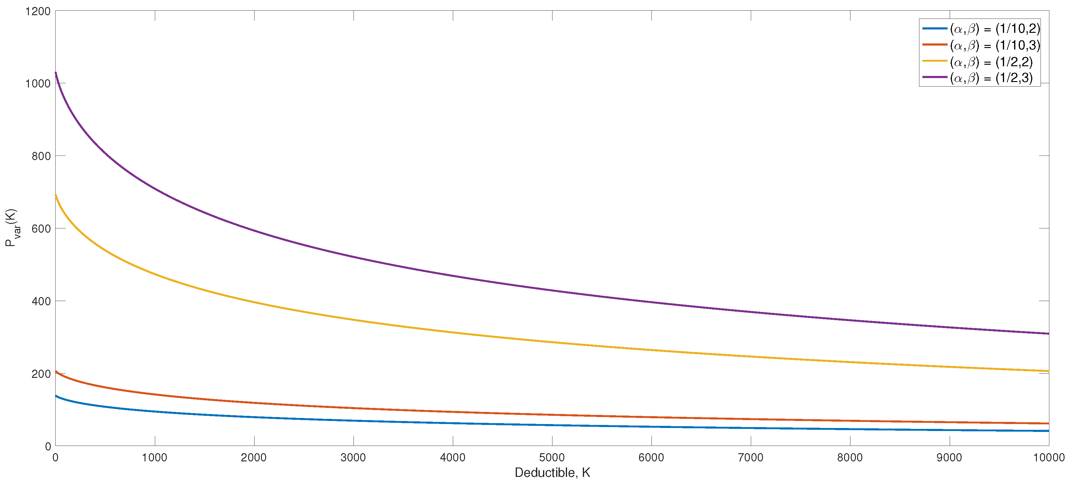
Hence, when the claims are log-normally distributed, the maximal premium that a customer with characteristics $(\alpha ,\beta )$ is willing to pay for an insurance contract as a function of the deductible is:

$$\begin{array}{cc}\hfill P_{\mathrm{var}}\left(K\right)=& \alpha K\overline{F}\left(K\right)\left(\frac{K\beta r}{2}-1\right)+\alpha \overline{z}\Phi \left(\frac{\mu +{\sigma }^2-log\left(K\right)}{\sigma }\right)(1-\beta rK)\hfill \\ & +\frac{\beta r\alpha \overline{z^2}}{2}\Phi \left(\frac{\mu +2{\sigma }^2-log\left(K\right)}{\sigma }\right).\hfill \end{array}$$

(14)

While this is not a straightforward expression, it is computationally easy to evaluate. Some combined data on claims in fire insurance reported 1958–1969 by Swedish fire insurance companies are studied in [15], where the estimates $\widehat{\mu }=1.6$ and $\widehat{\sigma }=1.99$ are obtained. These estimates are used in the following. In Figure 1, the premium function (14) for different combinations of characteristics is illustrated. The function appears to be very sensitive towards changes in characteristics and most so for small deductibles. Notice the considerable change from the combination $(\alpha ,\beta )=(1/10,2)$ to $(\alpha ,\beta )=(1/2,3)$ where the premium gets approximately 7.4-times larger.

Example 2.

An insurance company wants to supply fire insurance. It is entering a market where the customers have unknown, possibly different claim frequencies and constant risk aversions, namely β. The claim frequencies are once again assumed to be independent and identically exponentially distributed with parameter b. The portfolio can thus be characterized as in Section 3.1.

First, the insurer needs to see which region of the premium is profitable to even supply insurance. The criteria $p-\alpha (p,K)\overline{x^{\left(K\right)}}>0$ translates into:

$$p>\frac{2}{\beta rb}\frac{{\overline{x^{\left(K\right)}}}^2}{\overline{x^{2,\left(K\right)}}}+\frac{\overline{x^{\left(K\right)}}}{b}.$$

(15)

For a given deductible K, the considered price must exceed this threshold. Otherwise, the insurance company should choose not to supply insurance.

Next, evaluating the drift is of interest. Knowing the portfolio characteristics, it can be written explicitly as:

$$\mu (p;K)=Nexp\left(-b\frac{2p}{2\overline{x^{\left(K\right)}}+\beta r\overline{x^{2,\left(K\right)}}}\right)\left(p-\frac{2p\overline{x^{\left(K\right)}}}{2\overline{x^{\left(K\right)}}+\beta r\overline{x^{2,\left(K\right)}}}+\frac{\overline{x^{\left(K\right)}}}{b}\right)-L.$$

Solving the first order criteria (11) yields the solution:

$$\tilde{p}\left(K\right)=\frac{{(2\overline{x^{\left(K\right)}}+\beta r\overline{x^{2,\left(K\right)}})}^2}{2\beta br\overline{x^{2,\left(K\right)}}}=\frac{2}{\beta rb}\frac{{\overline{x^{\left(K\right)}}}^2}{\overline{x^{2,\left(K\right)}}}+\frac{\beta r\overline{x^{2,\left(K\right)}}}{2b}+\frac{2\overline{x^{\left(K\right)}}}{b}.$$

Notice that $\tilde{p}$ obviously satisfies being in the region of (15). We now seek to find the conditions under which the drift will be positive. Solving for $\mu (\tilde{p};K)>0$ yields:

$$\frac{L}{N}<\frac{\beta r\overline{x^{2,\left(K\right)}}}{2b}exp\left(-\frac{2\overline{x^{\left(K\right)}}+\beta r\overline{x^{2,\left(K\right)}}}{\beta r\overline{x^{2,\left(K\right)}}}\right).$$

Assuming that this inequality holds, then one must use Theorem 1 to find the optimal price. The optimality criterion in reduced form is:

$$\frac{N}{L}\frac{2\overline{x^{\left(K\right)}}+\beta r\overline{x^{2,\left(K\right)}}}{2b}=exp\left(\frac{2bp}{2\overline{x^{\left(K\right)}}+\beta r\overline{x^{2,\left(K\right)}}}\right)\frac{2bp}{2\overline{x^{\left(K\right)}}+\beta r\overline{x^{2,\left(K\right)}}}.$$

This yields the following optimal premium as a function of the deductible,

$$p^{*}\left(K\right)=\frac{2\overline{x^{\left(K\right)}}+\beta r\overline{x^{2,\left(K\right)}}}{2b}W\left(\frac{N}{L}\frac{2\overline{x^{\left(K\right)}}+\beta r\overline{x^{2,\left(K\right)}}}{2b}\right).$$

using the Lambert W function. The Lambert W function is defined as the (multivalued) inverse of the function $w\mapsto exp\left(w\right)w$. For more details, see [16]. In the case $\mu (\tilde{p};K)\le 0$, it follows from Theorem 2 that $\tilde{p}\left(K\right)$ is the optimal choice. Note that due to the Lambert W function increasing for positive values, then $p^{*}$ will be preferred to $\tilde{p}$ if $p^{*}\left(K\right)\ge \tilde{p}\left(K\right)$. Therefore, for a given deductible, K, it is preferable for the insurance firm to simply choose the maximum of $p^{*}\left(K\right)$ and $\tilde{p}\left(K\right)$.

Assume that the insurance company evaluates that the market consists of $N=10,000$ house owners considering buying insurance and that it calculated the liability costs to be $L=5000$. It also assesses that $b=3$ and $\beta =3$. Assume furthermore that the company has some information about the distribution of the claims, and based on this, it believes that the claims are log-normally distributed according to the estimates in [15]. It also knows how to reasonably choose a deductible K to serve the purpose described in the introduction. The interest rate applied is $2\%$.

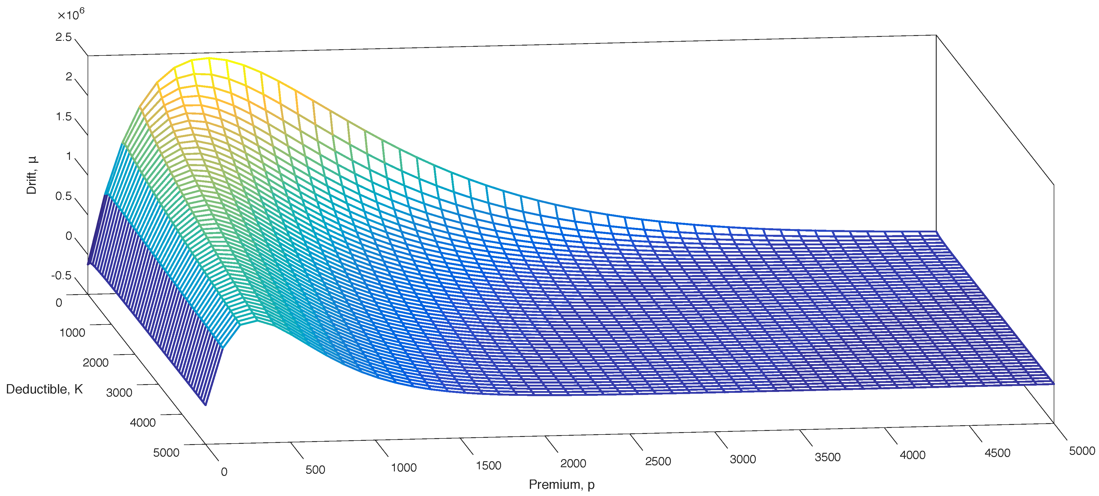
In Figure 2, a mesh of the drift is presented. The preliminary analysis of the drift in Section 4 is very well illustrated in this. The concavity in the premium is obvious. For all of the considered deductibles in the range $[0,5000]$, the drift will be positive in $\tilde{p}\left(K\right)$.

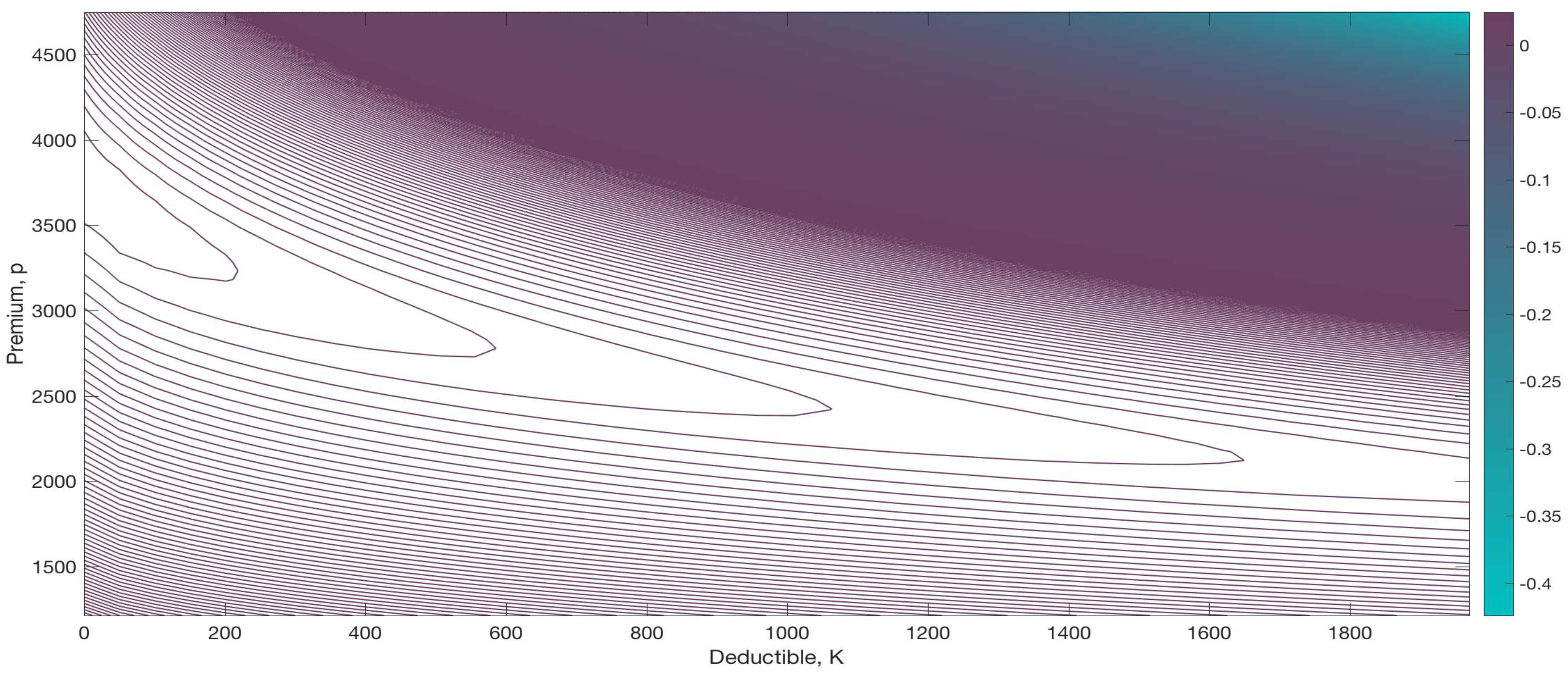
Next, a contour of the ratio $\mu /{\sigma }^2$ is illustrated in Figure 3. The concavity in the premium also appears very clearly here. The ratio is at its highest within the region of approximately $K\in [0,220]$, followed by the regions $K\in (220,590]$ and then $K\in (590,1070]$.

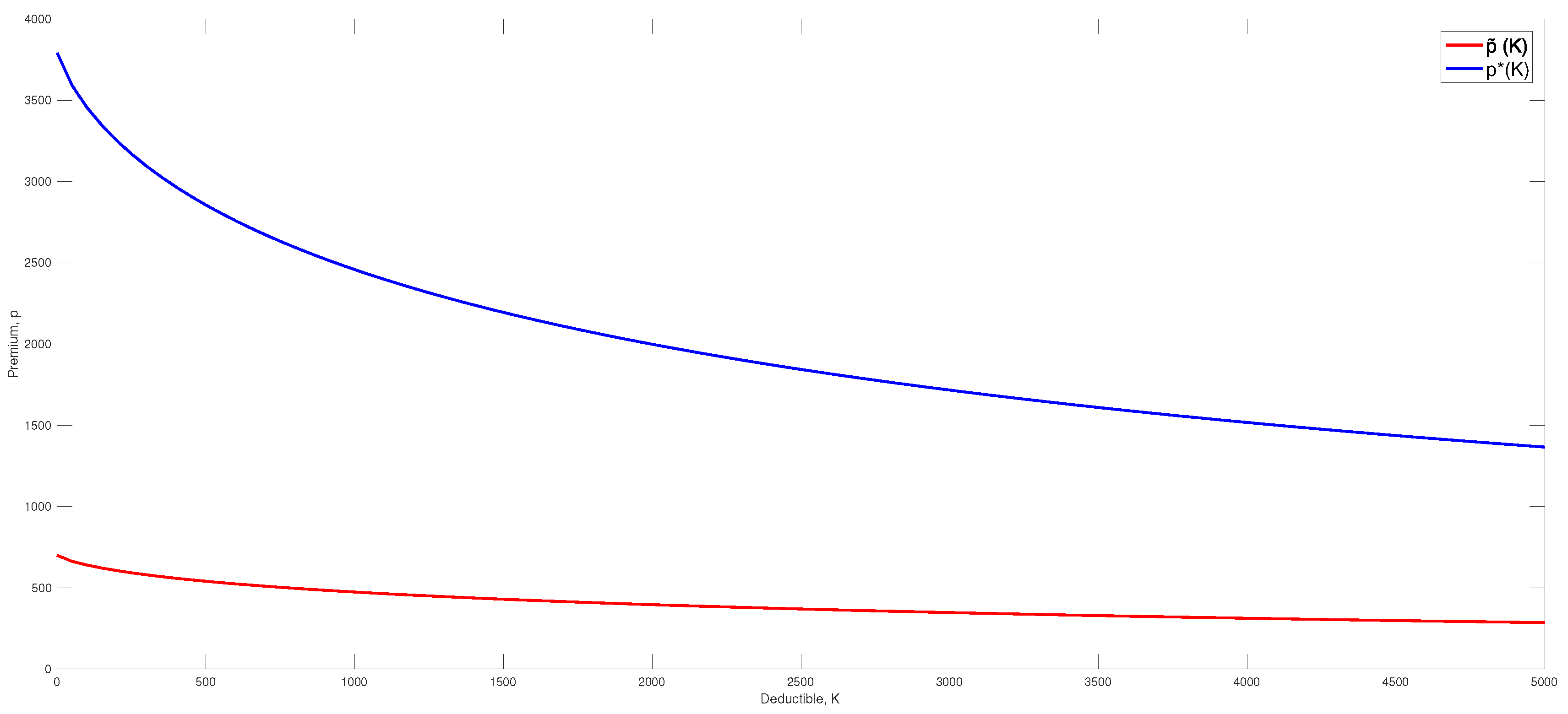
In Figure 4, the premiums $\tilde{p}\left(K\right)$ and $p^{*}\left(K\right)$ as functions of the deductible are plotted.

Notice that the model does not take the cost of processing an increasing number of claims into consideration. The company therefore evaluates that a deductible of $K=1000$ is suitable. This yields the following values:

$$\tilde{p}\left(1000\right)=474.2,p^{*}\left(1000\right)=2458.1,$$

Since $p^{*}\left(1000\right)>\tilde{p}\left(1000\right)$, then $p^{*}$ is the optimal premium.

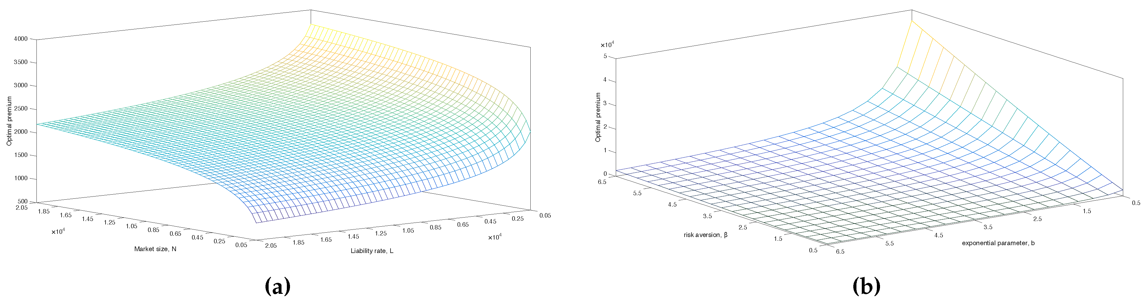
The optimal premium $max\{p^{*}\left(1000\right),\tilde{p}\left(1000\right)\}$ will of course depend on the parameters chosen, namely the market size N, the liability rate L, the risk aversion β and the exponential parameter b. An illustration of how sensitive the optimal premium are towards changes in these parameters is viewed in Figure 5. Figure 5a shows a mesh of the optimal premium where N and L take values in a grid of $[500,20,500]$. Here, we can see that the premium is most sensitive towards changes in these parameters for small values. A low liability rate L will yield a high premium. The insurance company does not need many customers when they have small liabilities payments; hence, they can afford to choose a high premium. On the contrary, when N is small, then we see that the premium tends to be low. In Figure 5b, a similar mesh of the optimal premium is shown for values of β and b in a grid of $[0.5,6.5]$. It is observed that when b gets too high or β too low, then the optimal premium will tend towards $\tilde{p}\left(1000\right)$. Conversely, when b takes on low values and β gets high, the optimal premium increases considerably. The values $N=10,000$, $L=5000$ $\beta =3$ and $b=3$ are chosen such that any of the extremes mentioned above are avoided.

Example 3.

Assume now that the insurance company believes that the claim frequency is constant in the portfolio, but does not possess any information about the customer’s risk aversion. The risk aversion is therefore modeled by a random variable, which is assumed to have an exponential distribution with parameter ν. Portfolio characteristics are then as in Section 3.2. The existence criteria of the insurance company will be $p-\alpha \overline{x^{\left(K\right)}}>0$, i.e., the premium must simply be larger than the net premium. First, we seek to find the solution of (11), namely:

$$\tilde{p}\left(K\right)=\frac{r\overline{x^{2,\left(K\right)}}\alpha }{2\nu }+\alpha \overline{x^{\left(K\right)}}.$$

Next is to find the region for which the drift evaluated in $\tilde{p}$ is positive:

$$\frac{L}{N}<\frac{r\overline{x^{2,\left(K\right)}}\alpha }{2\nu }exp(-1).$$

In this region:

$$p^{*}\left(K\right)=\frac{r\overline{x^{2,\left(K\right)}}\alpha }{2\nu }log\left(\frac{N}{L}\frac{r\overline{x^{2,\left(K\right)}}\alpha }{2\nu }\right)+\alpha \overline{x^{\left(K\right)}}$$

is optimal. Otherwise, $\tilde{p}$ is optimal. Again, due to the logarithm being an increasing function, one can simply state that the insurance company should choose the maximum of $\tilde{p}$ and $p^{*}$.