
Parameter Estimation in Stable Law

Institute of Mathematics and Statistics, University of Tartu, J. Liivi Str 2, Tartu 50409, Estonia
Risks 2016, 4(4), 43; https://doi.org/10.3390/risks4040043
Submission received: 22 September 2016
/
Revised: 7 November 2016
/
Accepted: 21 November 2016
/
Published: 25 November 2016
(This article belongs to the Special Issue Selected Papers from the 10th Tartu Conference on Multivariate Statistics)
Abstract
:For general stable distribution, cumulant function based parameter estimators are proposed. Extensive simulation experiments are carried out to validate the effectiveness of the estimates over the entire parameter space. An application to non-life insurance losses distribution is made.
1. Introduction
The four-parameter stable law arises as the limiting distribution of normalized sum of independent, identically distributed random variables. Stable distributions allow skewness and heavy tails and are proposed as models for various processes in physics, finance and elsewhere (see, e.g., [1]). However, modelling is complicated due to lack of a closed form for density of stable law. A number of parameter estimation techniques are based on the characteristic function. Regression-type characteristic function based methods are proposed in [2,3,4] and a minimum distance approach in [5]. Based on the logarithm of characteristic function, Press [6] proposes explicit point estimators for four parameters of stable law. His estimates depend on an arbitrary choice of two pairs of arguments of empirical characteristic function, and the method has not been recommended in practice. However, we found only a few papers (e.g, [5,7] for symmetric stable laws) introducing simulations on Press’s method while the optimal selection of arguments is still unresolved (for symmetric stable laws, some suggestions are given in [8]). In this paper, we show that the parameters of stable law can be expressed through cumulant function of one pair of arguments and hence the method of Press can be applied for one, not two pairs of arguments. We study the selection of arguments by an empirical search. To assess the effectiveness of estimates, we perform extensive simulations over the parameter space as well as present an application to non-life insurance losses.
The paper is organized as follows. In Section 2, we give some preliminary results about the stable laws. In Section 3, we discuss the main results on cumulant function based estimation. In Section 4, we present an empirical search for the selection of arguments, and in Section 5, we discuss simulations for a selected pair of arguments. Section 6 is devoted to an example in non-life insurance, and Section 7 provides conclusions.
2. Preliminaries
A random variable X is referred to as stable (see, e.g., [1,9,10]) if there exist constants and such that
where are independent random variables each having the same distribution as X. It has been shown (e.g., [1,11]) that in Equation (1), we have necessarily for some only. The variance of both sides of Equation (1) gives . For non-degenerate () distributions with finite variance, the index α must be equal to 2. If , the relation can be formally satisfied only with . Indeed, all stable distributions with have infinite variances, and when , they have an infinite mean as well. It is well known that normal (), Cauchy () and Levy () distributions belong to the class of stable laws. Naturally, α describes the rate of decay of the tails of stable distribution, the smaller the α, the slower is the decay and the heavier the tails. The parameter α is called a characteristic exponent, or index of stability. A skewness or asymmetry parameter characterizes the degree of asymmetry of the distributions being different from normal law (β is irrelevant when ). For , we have symmetric stable distributions and for totally skewed stable distributions. Like normal law, all stable distributions also remain stable under linear transformations, hence the scale parameter and the location parameter are introduced. It is worth mentioning that the scale parameter is not the standard deviation, and the location parameter is not generally the mean [e.g., [1,10]]. However, for we say standard stable distributions.
The density function of four-parameter stable distributions cannot be written analytically, and it is not as convenient to use as compared with characteristic (or cumulant) functions that also contain the complete information. The characteristic function of a stable random variable X is and the cumulant function is . The explicit representation of the characteristic (and cumulant) function of X depends on the parametrizations. In [1], several parametrizations are introduced while Nolan [10] proposes even more. Hence, when discussing the characteristic or cumulant function of stable law, the parametrization should always be stressed. Hereby, we denote [10] stable laws by , where 1 specifies the parametrization we use. The representation of characteristic function under 1-parametrization, similar to parametrization (A) in [1], is one of the most presented (as in [9], for example). The Definition 1 for the cumulant function of stable law follows the definition of 1-parametrization in [10].
Definition 1.
A random variable X is distributed according to distribution if
where Z is a random variable with cumulant function
where , , and , and . Then, X has the cumulant function
Our estimation procedure is based on the empirical cumulant function, i.e., on the logarithm of empirical characteristic function. For a sample of independent and identically distributed random variables, the empirical characteristic function is given as . It is easy to see that if are distributed as X, then . Hence, by the strong law of large numbers, the theoretical empirical characteristic function almost surely converges to the characteristic function for , i.e.,
and is a consistent estimator for . For studies on parameter estimation of stable laws based on empirical characteristic function, we refer, for example, to [2,3,4,5,6,7,8,12,13].
For a sample i.i.d. of random variables, the empirical cumulant function is
Complex numbers are complete metric space and the natural logarithm function is continuous; hence, as Equation (3) holds, then by continuous mapping theorem, see, e.g., [14]
and is a consistent estimator for . For more on the theory of empirical cumulant function based estimation, see, for example, [15].
3. Main Results
In this section, we introduce cumulant function estimation procedure. In Theorem 1, we show that the parameters of can be expressed through the cumulant function, and then, based on the empirical cumulant function, we propose the cumulant function based estimators.
Theorem 1.
Let . The parameters of can be expressed through the cumulant function (2) at ,
and in the case of
where α is given by Equation (6) and γ by Equation (7), and, in the case of
where γ is given by Equation (7), while Re, Im stand, respectively, for the real and imaginary parts of the cumulant function.
Proof.
Let us choose constants so that . Assuming that the parameters of a stable random variable are fixed, we can write the following system of equations:
As the system of Equation (12) is a system of complex numbers, it must simultaneously hold for real and imaginary parts of and . The real parts of and in Equation (12) give
Solving system (13) for α and γ gives Equations (6) and (7). The imaginary parts of and in (12) give two systems of equations. First, in the case of , the imaginary parts in Equation (12) give
Solving system (14) for δ and β gives Equations (8) and (9), where α and γ are solved from system (13) (and given by Equation (6) and Equation (7)). In the case of , the imaginary parts in Equation (12) give
Solving system (15) for δ and β gives the Equations (10) and (11) where γ is solved from Equation (13) and given by Equation (7). ☐
Next, we propose cumulant function based estimators. Techniques based on the logarithm of characteristic function are usually classified as characteristic function based methods. We, however, propose term cumulant estimators.
Definition 2.
If form a sample of independent and identically distributed random variables having the same distribution as , β, , and , then cumulant estimators
for the parameters of , β, are defined to satisfy Equations (6)–(11), where the real and imaginary parts of cumulant functions (2) are replaced with the real and imaginary parts of the empirical cumulant function (4).
As Equation (5) holds, then , and by continuous mapping theorem, see, e.g., [14], the cumulant estimators are consistent for the parameters of , β, (as also discussed in [6]).
Proposition 1.
The real and imaginary parts of empirical cumulant function (4) satisfy the representation’s = and =, where form a sample of i.i.d. random variables.
Proof.
From Euler’s formula, we have . The logarithm of a complex number is where and is calculated as arctangent function with two arguments (see, e.g., Kasana [16]), denoted by . Hence, the real and imaginary part of are as given in Proposition 1. ☐
It has been proposed to standardize the data with some estimates for the location δ and scale parameters γ before estimation procedure. Fama and Roll [17], and later [2,3] used the truncated sample mean for δ and sample quantiles for γ, while [4,5] proposed search methods for the initial estimates of δ and γ. However, we propose scaling by sample median, i.e., apply cumulant estimation procedure on the reduced (by sample median) data. For simplicity, we denote cumulant as well as reduced values’ cumulant estimators by , while the estimation method will be specified in context.
Definition 3.
Reduced values’ cumulant estimators for the parameters of , β, are defined through the cumulant estimators (Definition 2) on ,i.e., for the parameters of , where is the absolute value of the median of the sample i.i.d. random variables.
Note that reduced values’ cumulant estimators can only be used for samples with non-zero median.
Proposition 2.
If then for any ,
Proof.
The proof is based on the representation of the property of cumulant function, for any , . ☐
In the Section, following Section 4, we empirically search for the arguments for the estimators . In what follows, we discuss cumulant estimates, denoted by (not in bold), i.e., the non-random values computed on a particular realization of a sample i.i.d. random variables.
4. Empirical Search for the Optimal Arguments of Cumulant Estimators
Without loss of generality, we fix location parameter and scale parameter , i.e., study standard stable distributions and by reflection property (e.g., [1,10]) perform simulations for only. All simulations are carried out with package “stabledist” [18] in the open-source environment for statistical computing and graphics R [19].
Under each fixed , we simulate 200 realizations (replicates) of the sample , i.i.d stable random variables, , β, . For each replicate, we calculate the squared errors of cumulant and reduced values’ cumulant estimates at several selections of . We assess the quality of estimates to be the mean of squared errors (of 200 estimates), denoted by MSE (), MSE(), MSE(), and MSE().
In general, the selection of arguments is arbitrary. In our empirical search, we focus on pairs where the first argument is an arbitrary number on the order of magnitude , or 0, and the second argument is a multiple of the first argument. We present (and suggest) in Table 1 an arbitrary example of such set of pairs.
There is no specific reason for the selection of pairs in Table 1. We constructed (and performed simulations on) several similar sets, while in the main simulation used the set in Table 1. For the sake of space, we do not present all simulations (distributions) for pairs of arguments in Table 1. We will just choose four disparate standard stable distributions as examples. In Appendix A, the MSEs of reduced values’ estimates for , , and for the pairs of arguments are presented in Table 1. In addition, we do not present the MSEs of cumulant estimates, as in all cases they turned out higher than the MSEs of reduced values’ cumulant estimates. Naturally, for each stable law in Appendix A, there is a unique best (i.e., the values of MSE(), MSE(), MSE(), MSE( are lowest) pair of arguments. However, based on our empirical search (Appendix A and additional simulations), we propose the pair of as optimal (not necessarily the best).
Remark 1.
In our empirical search, we used the set of pairs arguments presented in Table 1 and proposed the pair of and as optimal.
In the remark, we accentuate and , as they are the only good pair of arguments for as well as giving MSEs less than 0.004 (at least) to all considered distributions. However, the quality of estimates may not be as good as for a single simulation as well as for real data. In Section 5, we present simulation over , at , , while in Section 6, for the application to non-life insurance losses, we use all the pairs of arguments in Table 1.
5. Simulations on the Effectiveness of Cumulant Estimates at
In this section, we present simulations to assess the effectiveness of at the selected pair of arguments (as proposed in Remark, Remark 1). We fix location parameter and scale parameter , and, by reflection property (e.g., [1,10]), perform simulations for only. Similarly to the previous section, under each fixed , we simulate 200 realizations (replicates). We simulate samples of sizes of , while, to save space, present the mean squared errors, MSE(), MSE(), MSE(), MSE(, for only. We note that the quality of estimates strongly depended on the sample size, as the smaller the sample, the lower the quality of estimates. All simulations are carried out with package “stabledist” [18] in the open-source environment for statistical computing and graphics R [19].
5.1. Simulations for
We present in the Appendix B the mean squared errors of cumulant (Definition 2) and of reduced values’ cumulant estimates (Definition 3) with in the cases of , , .
Remark 2.
The mean squared errors of reduced values’ estimates (at with ) for the parameters of in the cases of , , turned out to be on the order of magnitude (the values of MSE( were on the order of magnitude from to ).
Based on Appendix B and additional simulations (not presented here), we give the following remark.
Remark 3.
In our simulations, reduced values’ estimates turned out of better quality than cumulant estimates in the cases of and , while not in the cases of and .
5.2. Simulations in the Neighbourhood of
We study reduced values’ cumulant estimates in situations where the index of stability α is close to 1, i.e., , while . We present in Table 2 the mean squarer errors of some estimates where β was calculated by the Formulas (8), and (10) and δ was calculated by the Formulas (9) and (11).
It follows that reduced values’ cumulant estimates fail for the location parameter δ in the neighbourhood of . However, the estimates for other parameters are of better quality. Note that, for skewness parameter β, Formula (8) does not give better estimates than Formula (10), even if α is very close to 1. In addition, again, the MSEs of cumulant estimates (not presented here) were lower than reduced values’ cumulant estimates. In addition, we performed cumulant and reduced values’ cumulant estimates for all pairs of arguments given in Table 1. It follows that some other pairs of arguments (in Table 1) gave better estimates for the location parameter δ but concurrently fail in estimating the remaining parameters.
5.3. Simulations for
In Table 3, the MSEs of cumulant estimates for the case of and are presented. As in the estimation procedure, is not exactly 1. Then, for comparison, we present cumulant estimates for β with Formulas (8) and (10) and for δ with Formulas (9) and (11).
5.4. Simulations for and
In the case of , stable distributions are very condensed and scale factor γ has not much influence on the shape of the distribution (and may be difficult to estimate). We studied reduced values’ estimates for several cases of , . To save space, we do not present simulation results here. We will just summarise our findings by the following remarks.
Remark 4.
For (with ), MSE() and MSE() of reduced values’ estimates turned out to be on the order of magnitude from to , while the method fails for the scale parameter γ and (based on Equation (8)) for the skewness parameter β.
For the case of , it is discussed (see, e.g., [10,20]) that the value of β loses its effect (and may be difficult to estimate) as stable distributions get close to the normal distributions. We studied reduced values’ estimates for several cases of , and summarise our findings with the following remark.
Remark 5.
For (with ), the MSE(), MSE(), and MSE() of reduced values’ estimates turned out to be on the order of magnitude from to , while the method fails for the skewness parameter, β.
6. Application in Non-Life Insurance
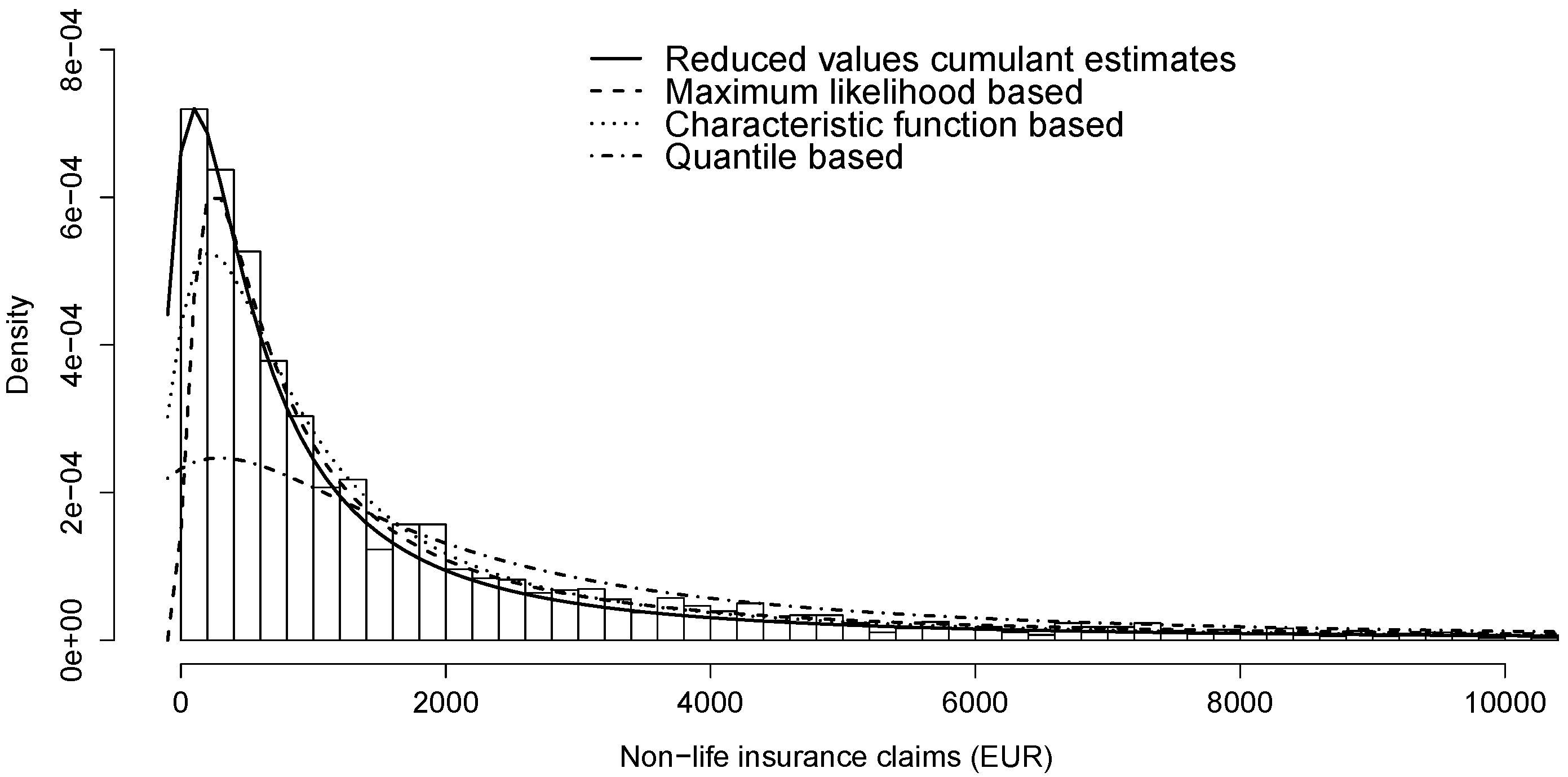
We consider an Estonian data set on fire, natural forces and other property insurance claim sizes of legal persons in a calendar year. The sample contains 2802 losses (EUR), and the summary statistics are in Table 4.
Based on the histogram of losses in Figure 1 and statistics in Table 4, the data is skewed, i.e., we expect the estimate for β to be close to 1. In addition, as the data is not condensed, it is natural to expect that estimates for α are not close to 0, as well as not close to 2 (claim sizes clearly are not normally distributed). We fit losses using cumulant and reduced values’ cumulant estimates for all pairs of arguments suggested in Table 1. Before estimating, we apply a simple non-parametric bootstrap with replacement.
6.1. Cumulant Estimates for Claim Sizes
We present in Table 5 the mean values of cumulant estimates for 200 bootstrap replicates. We remind readers that cumulant estimates are the same as Press’s [6] estimates, where we used the same pair of arguments for all parameters.
As previously discussed, the estimates for α should not be close to 0, while estimates for β should be close to 1. In addition, cumulant estimates for scale parameter γ turned out infinite (Inf). Hence, cumulant estimates in Table 5 are not meaningful, as also mentioned in [5] about Press’s [6] method.
6.2. Reduced Values’ Cumulant Estimates for Claim Sizes
We present in Table 6 the mean and coefficient of variation of reduced values’ cumulant estimates for 200 bootstrap replicates from claimsdata.
Table 6 is sorted increasingly by the variation of coefficient of . Reduced values’ estimates for the parameters of stable distribution in Table 6 are similar for several pairs of arguments. Based on the smallest coefficients of variation, we choose estimates at , , i.e., the stable distribution . However, similar to how it is discussed by Borak et al. [20] for Press”s [6] procedure, the optimal selection of arguments is still an open question. Clearly, optimal selection of and is related to scaling, i.e., reducing by the median. However, the relationship is not clear and needs further study.
6.3. Comparison to Other Estimation Methods
We compare the reduced values’ cumulant estimates with other commonly used estimation procedures, i.e., maximum likelihood method by Nolan [21], quantile based method by McCulloch [22] and empirical characteristic function based method by Koutrouvelis [2,3], and Kogon and Williams [4]. The estimates are performed with the STABLE program version, manufacturer,... (version 3.14.02, John P. Nolan, Washington, DC, USA) [23]. We present the estimated stable distributions in Table 7.
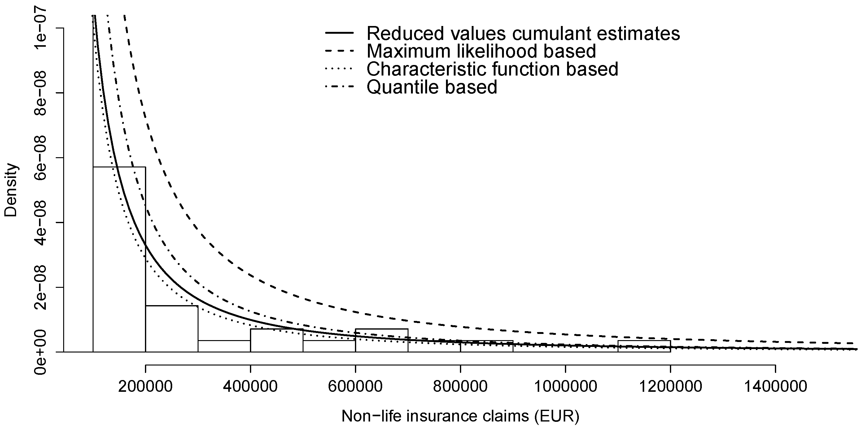
All estimation methods in Table 7 propose skewed stable distribution () with an index of stability less than 1 () and negative location parameter (). To illustrate the matches, we present in Figure 1 the histogram of losses and the density functions of stable distributions from Table 6. Densities in figures are numerically computed with package “stabledist” [18] in R [19].
We also present the tail behaviour in Figure 2. According to Figure 1 and Figure 2, the stable distribution estimated by reduced values’ cumulant estimates seem to match best with claims data. Naturally, the best fit should be measured with some goodness-of-fit test. In addition, as the estimated stable laws in Table 6 turned out different then our conclusions, similar to [24], more than one technique should be applied to fit any data with stable distributions.
7. Summary
In this paper we review the procedure of Press [6] for estimating the parameters of stable law. The method is based on cumulant function and leads explicit point estimators for all parameters. Press’s [6] estimates depend on an arbitrary choice of two pairs of arguments of empirical characteristic function, and it has not been recommended in practice. In this paper, we
- show that the parameters of stable law can be expressed through cumulant function of one pair of arguments, and hence
- propose the method of Press [6] at one pair of arguments only;
- suggest data scaling by median, i.e., introduce reduced values’ cumulant estimates;
- perform an empirical search for the selection of two arguments;
- carry out simulation experiments over parameter space at arguments of and ;
- present an application to non-life insurance losses;
According to our simulations reduced values’ estimates are of good quality for large samples () at empirically selected arguments of . In our simulations reduced values’ cumulant estimates turned out of better quality than Press’s [6] estimates at almost all empirically studied cases. Also, based on our application reduced values’ cumulant estimates can be suggested in practice.
An area for further research is to study the cumulant function based method under some other parametrization of stable laws, as well as some different shifting and scaling of data. Also, the cumulant function based method may be generalized to the multivariate case. Withal, the optimal selection of the two arguments still is an open question.
Acknowledgments
The author would like to thank the anonymous reviewers and editors for their useful comments and suggestions that greatly improved the quality of the paper. The author would like to express sincere gratitude to supervisor Tõnu Kollo for guidance, support and patience, and to John P. Nolan for helpful remarks. The author is thankful to Estonian Research Foundation for financial support from grant 9127 and the institutional research project IUT-34.
Conflicts of Interest
The author declares no conflict of interest.
Appendix A

Table A1.
The MSEs of reduced values’ cumulant estimates for the selection of for 200 replicates (sample size ) from .
| 0.03 | 0.03 | 0.03 | 0.03 | 0.3 | 0.3 | 0.3 | 0.3 | 3 | 3 | 3 | 3 | |
| 0.09 | 0.9 | 9 | 90 | 0.09 | 0.9 | 9 | 90 | 0.09 | 0.9 | 9 | 90 | |
| MSE () | 0.0000 | 0.0000 | 0.0059 | 0.0392 | 0.0000 | 0.0002 | 0.0163 | 0.0755 | 0.0007 | 0.0045 | 0.1520 | 0.2151 |
| MSE () | 0.0002 | 0.0001 | 0.0012 | 0.0091 | 0.0002 | 0.0007 | 0.0086 | 0.0311 | 0.0005 | 0.0231 | 4 × 101 | 3 × 101 |
| MSE () | 0.0001 | 0.0002 | 0.0425 | 0.3183 | 0.0001 | 0.0011 | 0.2077 | 7.7057 | 0.0002 | 0.1267 | Inf | Inf |
| MSE () | 0.0003 | 0.0000 | 0.0006 | 0.0000 | 0.0001 | 0.0002 | 0.0006 | 0.0000 | 0.0008 | 0.0030 | 0.0014 | 0.0000 |
| 0.03 | 0.03 | 0.03 | 0.03 | 0.3 | 0.3 | 0.3 | 0.3 | 3 | 3 | 3 | 3 | |
| 0.09 | 0.9 | 9 | 90 | 0.09 | 0.9 | 9 | 90 | 0.09 | 0.9 | 9 | 90 | |
| MSE () | 0.0001 | 0.0000 | 0.0000 | 0.0003 | 0.0000 | 0.0000 | 0.0000 | 0.0005 | 0.0000 | 0.0000 | 0.0001 | 0.0014 |
| MSE () | 0.0003 | 0.0001 | 0.0001 | 0.0043 | 0.0003 | 0.0002 | 0.0001 | 0.0146 | 0.0001 | 0.0002 | 0.0004 | 0.0993 |
| MSE () | 0.0036 | 0.0002 | 0.0002 | 0.0183 | 0.0012 | 0.0005 | 0.0002 | 0.0081 | 0.0001 | 0.0001 | 0.0003 | 0.0009 |
| MSE () | 0.0230 | 0.0006 | 0.0001 | 0.0218 | 0.0047 | 0.0013 | 0.0001 | 0.0235 | 0.0002 | 0.0004 | 0.0003 | 0.0318 |
| 0.03 | 0.03 | 0.03 | 0.03 | 0.3 | 0.3 | 0.3 | 0.3 | 3 | 3 | 3 | 3 | |
| 0.09 | 0.9 | 9 | 90 | 0.09 | 0.9 | 9 | 90 | 0.09 | 0.9 | 9 | 90 | |
| MSE () | 0.0001 | 0.3339 | 0.8957 | 1.2256 | 0.0933 | 2.2773 | 2.2475 | 2.2518 | 1.1632 | 2.2708 | 2.2755 | 2.2477 |
| MSE () | 0.0002 | 0.0414 | 0.0369 | 0.0594 | 0.2565 | 2 × 10² | 1 × 10² | 4 × 10² | 0.0653 | 2 × 10² | 2 × 10² | 4 × 10² |
| MSE () | 0.0000 | 0.1838 | 0.6175 | 0.8490 | 0.0056 | Inf | Inf | Inf | 1.0659 | Inf | Inf | Inf |
| MSE () | 0.0001 | 5 × 10³ | 0.0003 | 0.0000 | 8 × 101 | 0.1019 | 0.0004 | 0.0000 | 0.0029 | 0.0090 | 0.0010 | 0.0000 |
| 0.03 | 0.03 | 0.03 | 0.03 | 0.3 | 0.3 | 0.3 | 0.3 | 3 | 3 | 3 | 3 | |
| 0.09 | 0.9 | 9 | 90 | 0.09 | 0.9 | 9 | 90 | 0.09 | 0.9 | 9 | 90 | |
| MSE () | 0.0004 | 0.0001 | 0.1231 | 0.4640 | 0.0001 | 0.0000 | 0.3508 | 0.9181 | 0.0114 | 0.0928 | 2.2727 | 2.2629 |
| MSE () | 0.0011 | 0.0003 | 1.2741 | 1.9049 | 0.0002 | 0.0002 | 2.4033 | 4.4211 | 1.6320 | 5.1234 | 2 × 10² | 4 × 10² |
| MSE () | 0.0008 | 0.0000 | 0.3852 | 0.8615 | 0.0000 | 0.0000 | 0.1876 | 0.6170 | 0.0216 | 0.0039 | Inf | Inf |
| MSE () | 0.0003 | 0.0002 | 0.1416 | 0.0045 | 0.0002 | 0.0002 | 8.5030 | 0.0030 | 0.2452 | 5 × 101 | 0.0973 | 0.0005 |
Inf–infinity.
Appendix B
Table B1.
The MSEs of reduced values’ cumulant estimates (RVCE) and cumulant estimates (CE) at for 200 replicates (sample size ) from .
| α | β | Method | MSE () | MSE () | MSE () | MSE () |
|---|---|---|---|---|---|---|
| 0.25 | 0.1 | RVCE | 5.7 × 10⁻⁶ | 6.9 × 10⁻⁵ | 1.5 × 10⁻⁴ | 1.7 × 10⁻⁶ |
| 0.25 | 0.1 | CE | 3.8 × 10⁻⁵ | 6.3 × 10⁻⁴ | 5.5 × 10⁻³ | 5.5 × 10⁻³ |
| 0.25 | 0.25 | RVCE | 4.1 × 10⁻⁶ | 4.9 × 10⁻⁵ | 6.6 × 10⁻⁵ | 1.4 × 10⁻⁵ |
| 0.25 | 0.25 | CE | 3.5 × 10⁻⁵ | 4.6 × 10⁻⁴ | 4.6 × 10⁻³ | 4.6 × 10⁻³ |
| 0.25 | 0.5 | RVCE | 4.3 × 10⁻⁶ | 5.2 × 10⁻⁵ | 3.8 × 10⁻⁴ | 1.7 × 10⁻⁴ |
| 0.25 | 0.5 | CE | 3.9 × 10⁻⁵ | 6.1 × 10⁻⁴ | 5.8 × 10⁻³ | 5.8 × 10⁻³ |
| 0.25 | 0.75 | RVCE | 3.4 × 10⁻⁶ | 5.9 × 10⁻⁵ | 5.8 × 10⁻⁴ | 8.9 × 10⁻⁴ |
| 0.25 | 0.75 | CE | 3.6 × 10⁻⁵ | 6.1 × 10⁻⁴ | 5.4 × 10⁻³ | 5.4 × 10⁻³ |
| 0.25 | 1 | RVCE | 4.2 × 10⁻⁶ | 1.0 × 10⁻⁴ | 1.1 × 10⁻³ | 4.3 × 10⁻³ |
| 0.25 | 1 | CE | 4.3 × 10⁻⁵ | 7.1 × 10⁻⁴ | 6.3 × 10⁻³ | 6.3 × 10⁻³ |
| 0.5 | 0.1 | RVCE | 4.1 × 10⁻⁶ | 1.8 × 10⁻⁵ | 1.5 × 10⁻⁵ | 3.0 × 10⁻⁵ |
| 0.5 | 0.1 | CE | 4.6 × 10⁻⁵ | 3.2 × 10⁻⁴ | 4.3 × 10⁻³ | 4.3 × 10⁻³ |
| 0.5 | 0.25 | RVCE | 3.7 × 10⁻⁶ | 2.5 × 10⁻⁵ | 5.5 × 10⁻⁵ | 1.2 × 10⁻⁴ |
| 0.5 | 0.25 | CE | 6.7 × 10⁻⁵ | 2.4 × 10⁻⁴ | 3.6 × 10⁻³ | 3.6 × 10⁻³ |
| 0.5 | 0.5 | RVCE | 5.5 × 10⁻⁶ | 2.4 × 10⁻⁵ | 1.5 × 10⁻⁴ | 3.2 × 10⁻⁴ |
| 0.5 | 0.5 | CE | 5.8 × 10⁻⁵ | 2.6 × 10⁻⁴ | 4.4 × 10⁻³ | 4.4 × 10⁻³ |
| 0.5 | 0.75 | RVCE | 7.4 × 10⁻⁶ | 3.6 × 10⁻⁵ | 2.9 × 10⁻⁴ | 1.1 × 10⁻³ |
| 0.5 | 0.75 | CE | 5.5 × 10⁻⁵ | 2.8 × 10⁻⁴ | 6.1 × 10⁻³ | 6.1 × 10⁻³ |
| 0.5 | 1 | RVCE | 8.5 × 10⁻⁶ | 3.9 × 10⁻⁵ | 4.5 × 10⁻⁴ | 2.5 × 10⁻³ |
| 0.5 | 1 | CE | 5.5 × 10⁻⁵ | 3.0 × 10⁻⁴ | 8.4 × 10⁻³ | 8.4 × 10⁻³ |
| 0.75 | 0.1 | RVCE | 4.5 × 10⁻⁶ | 1.6 × 10⁻⁵ | 2.0 × 10⁻⁵ | 1.9 × 10⁻⁴ |
| 0.75 | 0.1 | CE | 9.9 × 10⁻⁵ | 3.1 × 10⁻⁴ | 7.3 × 10⁻³ | 7.3 × 10⁻³ |
| 0.75 | 0.25 | RVCE | 8.3 × 10⁻⁶ | 2.5 × 10⁻⁵ | 8.8 × 10⁻⁵ | 6.7 × 10⁻⁴ |
| 0.75 | 0.25 | CE | 1.2 × 10⁻⁴ | 3.1 × 10⁻⁴ | 9.6 × 10⁻³ | 9.6 × 10⁻³ |
| 0.75 | 0.5 | RVCE | 1.2 × 10⁻⁵ | 3.9 × 10⁻⁵ | 2.0 × 10⁻⁴ | 2.5 × 10⁻³ |
| 0.75 | 0.5 | CE | 9.9 × 10⁻⁵ | 2.5 × 10⁻⁴ | 1.7 × 10⁻² | 1.7 × 10⁻² |
| 0.75 | 0.75 | RVCE | 2.0 × 10⁻⁵ | 4.0 × 10⁻⁵ | 4.2 × 10⁻⁴ | 8.3 × 10⁻³ |
| 0.75 | 0.75 | CE | 9.5 × 10⁻⁵ | 2.3 × 10⁻⁴ | 2.8 × 10⁻² | 2.8 × 10⁻² |
| 0.75 | 1 | RVCE | 2.1 × 10⁻⁵ | 5.4 × 10⁻⁵ | 5.3 × 10⁻⁴ | 1.6 × 10⁻² |
| 0.75 | 1 | CE | 9.4 × 10⁻⁵ | 2.3 × 10⁻⁴ | 4.3 × 10⁻² | 4.3 × 10⁻² |
| 0.1 | RVCE | 5.8 × 10⁻⁶ | 1.5 × 10⁻⁵ | 5.7 × 10⁻⁶ | 5.7 × 10⁻⁵ | |
| 0.1 | CE | 3.2 × 10⁻⁴ | 8.5 × 10⁻⁴ | 1.4 × 10⁻³ | 1.4 × 10⁻³ | |
| 0.25 | RVCE | 1.8 × 10⁻⁵ | 3.9 × 10⁻⁵ | 4.3 × 10⁻⁵ | 1.3 × 10⁻⁴ | |
| 0.25 | CE | 4.1 × 10⁻⁴ | 1.0 × 10⁻³ | 2.7 × 10⁻³ | 2.7 × 10⁻³ | |
| 0.5 | RVCE | 3.8 × 10⁻⁵ | 7.8 × 10⁻⁵ | 1.5 × 10⁻⁴ | 4.0 × 10⁻⁴ | |
| 0.5 | CE | 4.3 × 10⁻⁴ | 7.7 × 10⁻⁴ | 4.8 × 10⁻³ | 4.8 × 10⁻³ | |
| 0.75 | RVCE | 5.6 × 10⁻⁵ | 1.4 × 10⁻⁴ | 3.0 × 10⁻⁴ | 8.9 × 10⁻⁴ | |
| 0.75 | CE | 4.0 × 10⁻⁴ | 7.2 × 10⁻⁴ | 7.9 × 10⁻³ | 7.9 × 10⁻³ | |
| 1 | RVCE | 8.8 × 10⁻⁵ | 1.3 × 10⁻⁴ | 5.5 × 10⁻⁴ | 1.9 × 10⁻³ | |
| 1 | CE | 3.8 × 10⁻⁴ | 6.0 × 10⁻⁴ | 1.2 × 10⁻² | 1.2 × 10⁻² | |
| 0.1 | RVCE | 3.8 × 10⁻⁶ | 1.8 × 10⁻⁵ | 1.2 × 10⁻⁶ | 1.2 × 10⁻⁵ | |
| 0.1 | CE | 5.9 × 10⁻⁴ | 1.9 × 10⁻³ | 2.2 × 10⁻⁴ | 2.2 × 10⁻⁴ | |
| 0.25 | RVCE | 5.0 × 10⁻⁶ | 2.2 × 10⁻⁵ | 2.9 × 10⁻⁶ | 1.2 × 10⁻⁵ | |
| 0.25 | CE | 6.0 × 10⁻⁴ | 2.0 × 10⁻³ | 2.4 × 10⁻⁴ | 2.4 × 10⁻⁴ | |
| 0.5 | RVCE | 1.6 × 10⁻⁵ | 4.7 × 10⁻⁵ | 1.7 × 10⁻⁵ | 1.8 × 10⁻⁵ | |
| 0.5 | CE | 6.2 × 10⁻⁴ | 1.9 × 10⁻³ | 2.6 × 10⁻⁴ | 2.6 × 10⁻⁴ | |
| 0.75 | RVCE | 2.4 × 10⁻⁵ | 7.4 × 10⁻⁵ | 4.0 × 10⁻⁵ | 2.3 × 10⁻⁵ | |
| 0.75 | CE | 5.6 × 10⁻⁴ | 1.9 × 10⁻³ | 3.3 × 10⁻⁴ | 3.3 × 10⁻⁴ | |
| 1 | RVCE | 3.4 × 10⁻⁵ | 9.8 × 10⁻⁵ | 6.9 × 10⁻⁵ | 3.2 × 10⁻⁵ | |
| 1 | CE | 5.9 × 10⁻⁴ | 1.7 × 10⁻³ | 3.9 × 10⁻⁴ | 3.9 × 10⁻⁴ | |
| 0.1 | RVCE | 8.3 × 10⁻⁴ | 4.7 × 10⁻³ | 4.6 × 10⁻⁵ | 4.6 × 10⁻⁵ | |
| 0.1 | CE | 4.5 × 10⁻² | 4.6 × 10⁻¹ | 1.2 × 10⁻³ | 4.2 × 10⁻¹ | |
| 0.25 | RVCE | 4.0 × 10⁻⁶ | 6.3 × 10⁻⁵ | 1.2 × 10⁻⁶ | 6.3 × 10⁻⁶ | |
| 0.25 | CE | 8.0 × 10⁻⁴ | 6.1 × 10⁻³ | 7.1 × 10⁻⁵ | 7.1 × 10⁻⁵ | |
| 0.5 | RVCE | 3.0 × 10⁻⁶ | 3.1 × 10⁻⁵ | 1.0 × 10⁻⁶ | 4.2 × 10⁻⁶ | |
| 0.5 | CE | 7.8 × 10⁻⁴ | 7.1 × 10⁻³ | 6.5 × 10⁻⁵ | 6.5 × 10⁻⁵ | |
| 0.75 | RVCE | 5.7 × 10⁻⁶ | 4.4 × 10⁻⁵ | 2.0 × 10⁻⁶ | 4.6 × 10⁻⁶ | |
| 0.75 | CE | 7.6 × 10⁻⁴ | 7.4 × 10⁻³ | 5.8 × 10⁻⁵ | 5.8 × 10⁻⁵ | |
| 1 | RVCE | 8.1 × 10⁻⁶ | 9.1 × 10⁻⁵ | 3.4 × 10⁻⁶ | 5.2 × 10⁻⁶ | |
| 1 | CE | 9.7 × 10⁻⁴ | 9.4 × 10⁻³ | 7.3 × 10⁻⁵ | 7.3 × 10⁻⁵ |
References
- V.V. Uchaikin, and M.V. Zolotarev. Chance and Stability: Stable Distributions and Their Applications. Utrecht, The Netherland: Walter de Gruyter, 1999. [Google Scholar]
- I.A. Koutrouvelis. “Regression-type estimation of the parameters of stable laws.” J. Am. Stat. Assoc. 75 (1980): 918–928. [Google Scholar] [CrossRef]
- I.A. Koutrouvelis. “An iterative procedure for estimation of the parameters of stable laws.” Commun. Statist. Simul. Comput. 10 (1981): 17–28. [Google Scholar] [CrossRef]
- S.M. Kogon, and D.B. Williams. “Characteristic function based estimation of stable parameters.” In A Practical Guide to Heavy Tails. Edited by R. Adler, R. Feldman and M. Taqqu. Boston, MA, USA: Birkhäuser, 1998, pp. 311–335. [Google Scholar]
- A.S. Paulson, E.W. Holcomb, and R.A. Leitch. “The estimation of the parameters of the stable laws.” Biometrika 62 (1975): 163–170. [Google Scholar] [CrossRef]
- S.J. Press. “Estimation in univariate and multivariate stable distribution.” J. Am. Stat. Assoc. 67 (1972): 842–846. [Google Scholar] [CrossRef]
- Z. Fan. “Parameter Estimation of Stable Distributions.” Commun. Stat. Theory Methods 35 (2006): 245–255. [Google Scholar] [CrossRef]
- R. Höpfner, and L. Rüschendorf. “Comparison of estimators in stable models.” Math. Comput. Model. 29 (1999): 145–160. [Google Scholar] [CrossRef]
- G. Samorodnitsky, and M.S. Taqqu. Stable Non-Gaussian Random Processes: Stochastic Models with Infinite Variance. New York, NY, USA: Chapman and Hall/CRC, 1994. [Google Scholar]
- J.P. Nolan. Stable Distributions - Models for Heavy Tailed Data. Boston, MA, USA: Birkhäuser, 2016, Chapter 1; Available online: http://fs2.american.edu/jpnolan/www/stable/chap1.pdf (accessed on 23 September 2015).
- W. Feller. An introduction to Probability Theory and its Applications, 2nd ed. New York, NY, USA: Wiley, 1971, Volume 2. [Google Scholar]
- C. Heathcote. “The Integrated Squared Error Estimation of Parameters.” Biometrika 64 (1977): 255–264. [Google Scholar] [CrossRef]
- J. Yu. “Empirical Characteristic Function Estimation and Its Applications.” Econometr. Rev. 23 (2004): 93–123. [Google Scholar] [CrossRef]
- A.W. Van der Vaart. Asymptotic Statistics. New York, NY, USA: Cambridge University Press, 1998. [Google Scholar]
- J.L. Knight, and S.E. Satchell. “The Cumulant Generating Function Estimation Method.” Econometr. Theory 13 (1997): 170–184. [Google Scholar] [CrossRef]
- H.S. Kasana. Complex Variables: Theory And Applications, 2nd ed. New Delhi, India: Prentice-Hall of India Private Limited, 2005. [Google Scholar]
- E.F. Fama, and R. Roll. “Parameter estimates for symmetric stable distributions.” J. Am. Stat. Assoc. 66 (1978): 331–338. [Google Scholar] [CrossRef]
- D. Wuertz, and M. Maechler. Rmetrics Core Team Members Stabledist: Stable Distribution Functions, R Package Version 0.7-0; 2015. Available online: https://CRAN.R-project.org/package=stabledist (accessed on 20 January 2016).
- R Core Team. R: A language and environment for statistical computing. Vienna, Austria: R Foundation for Statistical Computing, 2015, Available online: http://www.R-project.org/ (accessed on 20 January 2016).
- S. Borak, K.W. Härdle, and R. Weron. “Stable Distributions.” In Statistical Tools for Finance and Insurance. Edited by P. Čižek, K.W. Härdle and R. Weron. Berlin, Germany: Springer, 2005, pp. 21–45. [Google Scholar]
- J.P. Nolan. “Maximum likelihood estimation and diagnostic for stable distributions.” In Lévy Processes. Edited by O.E. Barndorff-Nielsen, T. Mikosh and S. Resnick. Boston, MA, USA: Birkhäuser, 2001, pp. 379–400. [Google Scholar]
- J.H. McCullogh. “Simple consistent estimators of stable distributions parameters.” Commun. Stat. Simul. 15 (1986): 1109–1136. [Google Scholar] [CrossRef]
- J.P. Nolan. STABLE Program for Windows Version 3.14.02. 2005. Available online: http://academic2.american.edu/~jpnolan/stable/stable.html (accessed on 15 February 2016).
- S. Bates, and S. McLaughlin. “The estimation of stable distribution parameters.” In Proceedings of the IEEE Signal Processing Workshop on in Higher-Order Statistics; Chicago, IL, USA: IEEE Press, 1997, pp. 390–394. [Google Scholar]
Figure 1.
Modelling non-life insurance losses () via stable distributions (Table 6).
Figure 1.
Modelling non-life insurance losses () via stable distributions (Table 6).

Figure 2.
Modelling non-life insurance losses () via stable distributions (Table 6).
Figure 2.
Modelling non-life insurance losses () via stable distributions (Table 6).

| Argument | Values | |||||||||||
|---|---|---|---|---|---|---|---|---|---|---|---|---|
| 0.03 | 0.03 | 0.03 | 0.03 | 0.3 | 0.3 | 0.3 | 0.3 | 3 | 3 | 3 | 3 | |
| 0.09 | 0.9 | 9 | 90 | 0.09 | 0.9 | 9 | 90 | 0.09 | 0.9 | 9 | 90 | |
| Formula | (8) | (10) | (9) | (11) | |||
|---|---|---|---|---|---|---|---|
| MSE () | MSE () | MSE () | MSE () | MSE () | MSE () | ||
| 0.95 | 0.1 | 0.0000 | 0.0001 | 0.0003 | 0.0000 | 0.0458 | 1.6567 |
| 0.95 | 1 | 0.0003 | 0.0008 | 0.0688 | 0.0023 | 9 × 101 | 2 × 10² |
| 0.96 | 0.1 | 0.0000 | 0.0001 | 0.0002 | 0.0001 | 0.1537 | 2.6231 |
| 0.96 | 1 | 0.0005 | 0.0012 | 0.0496 | 0.0044 | 5 × 10⁴ | 3 × 10² |
| 0.98 | 0.1 | 0.0001 | 0.0002 | 0.0003 | 0.0003 | 7 × 101 | 1 × 101 |
| 0.98 | 1 | 0.0009 | 0.0027 | 0.0309 | 0.0135 | 4 × 10⁵ | 1 × 10³ |
| 0.99 | 0.1 | 0.0002 | 0.0005 | 0.0005 | 0.0007 | 1 × 10⁶ | 4 × 101 |
| 0.99 | 1 | 0.0017 | 0.0045 | 0.0553 | 0.0333 | 2 × 10⁴ | 4 × 10³ |
| 1.01 | 0.1 | 0.0002 | 0.0004 | 0.0004 | 0.0007 | 2 × 10⁵ | 4 × 101 |
| 1.01 | 1 | 0.0016 | 0.0060 | 0.0383 | 0.0278 | 4 × 10⁶ | 4 × 10³ |
| 1.02 | 0.1 | 0.0001 | 0.0002 | 0.0002 | 0.0002 | 1 × 10³ | 1 × 101 |
| 1.02 | 1 | 0.0009 | 0.0027 | 0.0202 | 0.0108 | 4 × 10⁴ | 9 × 10² |
| 1.04 | 0.1 | 0.0001 | 0.0001 | 0.0002 | 0.0001 | 0.1101 | 2.4367 |
| 1.04 | 1 | 0.0006 | 0.0015 | 0.0340 | 0.0046 | 2 × 10⁴ | 2 × 10² |
| 1.05 | 0.1 | 0.0000 | 0.0001 | 0.0001 | 0.0000 | 0.0458 | 1.5814 |
| 1.05 | 1 | 0.0005 | 0.0013 | 0.0392 | 0.0032 | 3 × 10² | 1 × 10² |
| Formula | (8) | (10) | (9) | (11) | ||
|---|---|---|---|---|---|---|
| MSE () | MSE () | MSE () | MSE () | MSE () | MSE () | |
| 0.1 | 0.0002 | 0.0004 | 0.0004 | 0.0013 | 5 × 101 | 0.0012 |
| 0.25 | 0.0002 | 0.0609 | 0.0609 | 0.0216 | 3 × 10³ | 0.0072 |
| 0.5 | 0.0002 | 0.2421 | 0.2422 | 0.0348 | 2 × 101 | 0.0430 |
| 0.75 | 0.0002 | 0.5476 | 0.5473 | 0.0443 | 1 × 10³ | 0.0938 |
| 1 | 0.0002 | 0.9717 | 0.9713 | 0.3854 | 5 × 10³ | 0.1925 |
| Min | 1st Quartile | Median | Mean | 3rd Quartile | Maximum |
|---|---|---|---|---|---|
| 15.3 | 358.0 | 955.0 | 6703.0 | 2781.0 | 1166000.0 |
| Mean () | Mean () | Mean () | Mean () | ||
|---|---|---|---|---|---|
| 0.03 | 0.09 | 0.13 | 1.62 | 9 × 1077 | –3.77 |
| 0.03 | 0.9 | 0.01 | 6.70 | Inf | 1.53 |
| 0.03 | 9 | 0.03 | 2.98 | Inf | –0.10 |
| 0.03 | 90 | 0.02 | –0.76 | Inf | –0.02 |
| 0.3 | 0.09 | 0.04 | –0.42 | Inf | 3.05 |
| 0.3 | 0.9 | –0.17 | –1.22 | Inf | 1.93 |
| 0.3 | 9 | –0.01 | –1.46 | Inf | –0.17 |
| 0.3 | 90 | –0.01 | 0.79 | Inf | –0.02 |
| 3 | 0.09 | 0.01 | –2.35 | Inf | 0.12 |
| 3 | 0.9 | 0.14 | 2.18 | 3 × 10125 | –0.87 |
| 3 | 9 | –0.04 | 0.36 | 5× 10184 | –0.29 |
| 3 | 90 | –0.03 | 0.59 | Inf | –0.02 |
Inf–infinity.
| Mean | CV | Mean | CV | Mean | CV | Mean | CV | ||
|---|---|---|---|---|---|---|---|---|---|
| () | () | () | () | () | () | () | () | ||
| 0.03 | 9 | 0.71 | 0.030 | 1.19 | 0.059 | 382.46 | 0.073 | –432.25 | 0.206 |
| 3 | 0.09 | 0.72 | 0.030 | 1.12 | 0.042 | 444.48 | 0.045 | –574.15 | 0.209 |
| 0.3 | 9 | 0.67 | 0.032 | 1.17 | 0.046 | 410.33 | 0.059 | –335.48 | 0.181 |
| 0.03 | 0.9 | 0.77 | 0.039 | 1.05 | 0.057 | 568.07 | 0.057 | –1113.55 | 0.328 |
| 0.03 | 90 | 0.56 | 0.039 | 1.78 | 0.079 | 119.88 | 0.192 | –103.29 | 0.181 |
| 0.3 | 0.9 | 0.80 | 0.048 | 1.06 | 0.055 | 578.91 | 0.059 | –1460.33 | 0.342 |
| 0.3 | 90 | 0.48 | 0.058 | 1.87 | 0.085 | 181.45 | 0.175 | –85.05 | 0.183 |
| 3 | 0.9 | 0.60 | 0.064 | 1.18 | 0.061 | 475.25 | 0.046 | –283.09 | 0.345 |
| 0.3 | 0.09 | 0.75 | 0.069 | 1.00 | 0.072 | 523.66 | 0.145 | –819.13 | 0.793 |
| 0.03 | 0.09 | 0.78 | 0.099 | 1.09 | 0.101 | 581.48 | 0.304 | –1989.91 | 1.272 |
| 3 | 9 | 0.60 | 0.107 | 0.94 | 0.133 | 484.41 | 0.092 | –139.00 | 0.608 |
| 3 | 90 | 0.33 | 0.151 | 2.00 | 0.157 | 690.79 | 0.194 | –60.62 | 0.204 |
CV–coefficient of variation.
© 2016 by the author; licensee MDPI, Basel, Switzerland. This article is an open access article distributed under the terms and conditions of the Creative Commons Attribution (CC-BY) license (http://creativecommons.org/licenses/by/4.0/).
Share and Cite
MDPI and ACS Style
Krutto, A. Parameter Estimation in Stable Law. Risks 2016, 4, 43. https://doi.org/10.3390/risks4040043
AMA Style
Krutto A. Parameter Estimation in Stable Law. Risks. 2016; 4(4):43. https://doi.org/10.3390/risks4040043
Chicago/Turabian StyleKrutto, Annika. 2016. "Parameter Estimation in Stable Law" Risks 4, no. 4: 43. https://doi.org/10.3390/risks4040043
Note that from the first issue of 2016, this journal uses article numbers instead of page numbers. See further details here.