Article

Optimal Reinsurance Under General Law-Invariant Convex Risk Measure and TVaR Premium Principle

1
School of Mathematics and Computer Science & FJKLMAA, Fujian Normal University, Fuzhou 350108, China
2
School of Mathematical Sciences, Xiamen University, Xiamen 361005, Fujian, China
3
School of Statistics and Mathematics, ZheJiang GongShang University, Hangzhou 310018, China
4
School of Applied Mathematics, Xinjiang University of Finance and Economics, Urumchi 830012, Xinjiang, China
*
Author to whom correspondence should be addressed.
Risks 2016, 4(4), 50; https://doi.org/10.3390/risks4040050
Submission received: 13 June 2016 / Revised: 2 December 2016 / Accepted: 9 December 2016 / Published: 16 December 2016

Abstract

:
In this paper, we study the optimal reinsurance problem where risks of the insurer are measured by general law-invariant risk measures and premiums are calculated under the TVaR premium principle, which extends the work of the expected premium principle. Our objective is to characterize the optimal reinsurance strategy which minimizes the insurer’s risk measure of its total loss. Our calculations show that the optimal reinsurance strategy is of the multi-layer form, i.e., f * ( x ) = x c * + ( x - d * ) + with c * and d * being constants such that 0 c * d * .

1. Introduction

The issue of optimal reinsurance design has recently aroused great interests from mathematicians in both academia and the financial industry. A reinsurance policy is a contract, according to which the reinsurance company covers part of the risk of an insurance (or, ceding) company, in exchange for receiving a premium calculated under some premium principle. It’s seen that identifying the criterion that is applied to get an optimal reinsurance strategy is the cornerstone of reinsurance optimization. It is well known that there have been several criterions of reinsurance optimization in the literature. The first and most classical optimization criterion is variance minimization. It is shown that the pure stop-loss reinsurance is the optimal reinsurance strategy because of the smallest variance of the insurer’s retained loss among all the strategies with the same pure premium, see, Borch [1], Kaluszka [2], Kaas, et al. [3], and so on. The second one is utility maximization, which is attributed to Arrow [4]. It asserts that the stop-loss reinsurance maximizes the expected utility of the insurer, provided that the insurer has a concave utility function. Other criterions such as “maximizing the joint survival probability”, “minimizing the risk-adjusted value” and “behavioral criterion” for example the disappointment theory related criterion, have also featured in some existing works. See, for instance, Cai, et al. [5], Chi [6] and Cheung, et al. [7]. Recently, the optimization criterion of minimization of a number of ingenious risk measures is also widely applied, see Kaluszka [8,9], Gajek and Zagrodny [10], Promislow and Young [11], Cai, et al. [12], Balbás, et al. [13], Cheung [14], Chi and Weng [15] and the references therein.
In this paper, the “risk measure minimization” optimization criterion is considered. Under the “risk measure minimization” criterion the body of literature regarding the optimal reinsurance strategy has been witnessing the following four directions of generalization from the mathematics aspect.
(a)
Generalizing the set of ceded loss functions. Cai, et al. [12] and Cheung [14] considered the set of all the increasing and convex functions as their feasible ceded loss function class. While, Lu, et al. [16] took the set of all the increasing and concave functions as their feasible ceded loss function class. Chi and Weng [15] extended their feasible ceded loss function class to
{ f ( x ) | 0 f ( x ) x , both x f ( x ) and f ( x ) / x   are   increasing   function   of   x } .
Chi and Tan [17] further extended their feasible ceded loss function class to
{ f ( x ) | 0 f ( x ) x , both x f ( x ) and f ( x ) are   increasing   function   of   x } .
Other more general feasible ceded loss function class
{ f ( x ) | 0 f ( x ) x , x f ( x ) ( or f ( x ) ) is   increasing   ( left-continuous )   function   of   x }
can be found in Cheung and Lo [18]. Different reinsurance contracts have been introduced in the reinsurance market among which there are quota-share, stop-loss, stop-loss after quota-share and quota-share after stop-loss, etc. It can be verified that all these reinsurance contracts belong to some or all of the above-mentioned feasible ceded loss function classes.
(b)
Generalizing the premium principles. To our knowledge, the most widely used premium principle in the existing works turns out to be the expected premium principle, see Cheung, et al. [19], Lu, et al. [16], Cai, et al. [5], Chi and Tan [17], etc.. Assa [20], Zheng and Cui [21], Cui, et al. [22] extended their premium principle to the distortion premium principle. Zhu, et al. [23] further extended their premium principle to very general one that satisfies three mild conditions: distribution invariance, risk loading and preserving the convex order, see also Chi and Tan [24].
(c)
Generalizing the risk measures. Using the VaR, CTE, AVaR, respectively, Hu, et al. [25], Cai and Tan [26], Cai, et al. [12], Cheung [14] and Chi and Tan [24] found the optimal reinsurance contract. In Asimit, et al. [27], a quantile-based risk measure was adopted in accordance with the insurer’s appetite. Assa [20], Zheng and Cui [21] and Cui, et al. [22] generalized their risk measures to the distortion risk measures. Cheung, et al. [19] further extended the problem by using a general law-invariant convex risk measure.
(d)
Constraints involved. Borch [1] (and also Arrow [4]) showed that, subject to a budget constraint, the stop-loss policy is an optimal reinsurance contract for the ceding company when the risk is measured by variance (or by a utility function). Reinsurance optimization problems involving premium constraint were also considered in Gajek and Zagrodny [10], Zhou, et al. [28], Zheng and Cui [21], Cui, et al. [22] and Cheung and Lo [18]. Cheung, et al. [29] introduced a reinsurer’s probabilistic benchmark constraint of his potential loss. In Tan and Weng [30], a profitability constraint was proposed.
Inspired by the above four directions of generalization, this paper extends the work of Cheung, et al. [19] from the expected premium principle to the TVaR premium principle, which was first proposed in Young [31] (see also, Kaluszka [9]). The optimal reinsurance problem under the general law-invariant convex risk measures with premiums being calculated according to the TVaR premium principle is considered. The optimal reinsurance strategy which minimizes the insurer’s risk measure of its total loss is characterized. By constraining the ceded loss function class to be the set of 1-Lipschitz continuous functions, the optimal reinsurance strategy is of the form f * ( x ) = x c * + ( x d * ) + with 0 c * d * .
The rest of the paper is organized as follows. Section 2 gives the mathematical presentation of our reinsurance optimization problem. The optimal reinsurance strategy is characterized in Section 3. In Section 4 some sensitivity analysis is carried out for the optimal value function given by (2) (see Section 2), where two particular scenarios of Problem (2) (see Section 2) are considered.

2. The Mathematical Presentation of the Reinsurance Optimization Problem

Suppose that the probability space ( Ω , F , P ) carries all the random arguments concerned in the sequel. Let X be a nonnegative random variable defined on ( Ω , F , P ) , representing the amount of claims in a fixed time period. We also suppose that an insurance company which is exposed to the risk X decides to purchase a reinsurance policy, and f ( X ) is the part of loss transferred from the insurer to the reinsurer, the insurer’s retained loss thus is X f ( X ) . Here, the function f : [ 0 , ) [ 0 , ) is said to be a ceded loss function or an indemnification function. The reinsurance premium charged by the reinsurer for taking up the loss f ( X ) is assumed to be calculated according to the so-called TVaR premium principle with level parameter β ( 0 , 1 ] and safety loading coefficient θ 0 , i.e.,
μ ( f ( X ) ) = ^ 1 + θ β 0 β S f ( X ) 1 ( x ) d x with S Y 1 ( x ) = ^ inf { y 0 | S Y ( y ) x } .
Here, S X ( y ) = ^ 1 F X ( y ) = ^ P ( X > y ) is the tail distribution of X. Such a premium principle was first proposed by Young [31] (see also, Kaluszka [9]). It can be viewed as an extended version of the expected premium principle, that is, letting β = 1 in (1) gives the expected premium principle. Consequently, the total cost of the insurer under the reinsurance arrangement is given by X f ( X ) + μ ( f ( X ) ) , and the corresponding cost of the reinsurer is given by f ( X ) μ ( f ( X ) ) . To avoid tedious discussions and arguments, we assume further that the distribution function of X, say F X ( y ) , is continuous on [ 0 , ) with F X ( 0 ) = 0 .
The objective of this paper is to determine the optimal design of reinsurance contracts so that the insurer’s risk exposure, measured by a general law-invariant convex risk measure, can be minimized. Specifically, we focus on the following problem
inf f H ρ X f ( X ) + μ ( f ( X ) ) ,
where H is the following admissible ceded loss function set
H = ^ { f 0 f ( x ) x , f ( x )   and   x f ( x )   are   nondecreasing   functions   of   x } ,
ρ is the general law-invariant convex risk measure adopted by the insurer. According to Föllmer and Schied [32] it has a representation of the following form
ρ ( Y ) = sup ν M 1 ( 0 , 1 ] A V a R α ( Y ) ν ( d α ) ψ ( ν ) ,
here M 1 is the set of all probability measures on ( 0 , 1 ] , ψ : M 1 R is a functional, and A V a R α is the average value at risk (risk measure) with level parameter α,
A V a R α ( Y ) = ^ 1 α 0 α V a R λ ( Y ) d λ ,
with Y being any wealth random variable, and V a R α ( Y ) = S Y 1 ( α ) is the V a R risk measure. Hence, the so-called TVaR premium principle introduced in Young [31] (see also, Kaluszka [9]) equals, up to multiplication by the constant 1 + θ , to the A V a R β risk measure of f ( X ) . That is, we have μ ( f ( X ) ) = ( 1 + θ ) A V a R β ( f ( X ) ) .
It can be seen that the AVaR (hence the TVaR) measures average losses in the most adverse cases rather than just the minimum loss, as the VaR does. Therefore, calculating premiums by the TVaR has two advantages: (a) unlike the expected premium principle, premiums for catastrophic losses are taken into account well enough by AVaR and hence underestimation of premiums is avoided; (b) TVaR has the subadditivity property, while the subadditivity is an appealing property when aggregating risks in order to preserve the benefits of diversification. Hence, the TVaR would appear to be a more powerful premium principle for assessing the actual risks faced by the reinsurance companies. For more detailed information about TVaR (AVaR) please refer to Belles-Sampera, et al. [33].
It is necessary to claim that the ceded loss function class H consists of all 1-Lipschitz continuous functions. In fact, the nondecreasing property of f ( x ) results in 0 f ( x ) f ( y ) , while the nondecreasing property of x f ( x ) results in y f ( y ) x f ( x ) f ( x ) f ( y ) x y for all 0 y x .

3. Characterizing the Optimal Reinsurance Strategy

As a transition, we first study the following optimal reinsurance problem
inf f H A V a R α { X f ( X ) + 1 + θ β 0 β S f ( X ) 1 ( x ) d x } .
By the definition of S X 1 ( x ) in the latter equality of Equation (1), we have
S X 1 ( α ) > x S X ( x ) > α , S X 1 ( α ) x S X ( x ) α , S X ( S X 1 ( α ) ) α .
In addition, for any continuous nondecreasing function f, we have
S f ( X ) 1 ( α ) = f ( S X 1 ( α ) ) .
See, Equation (2.2) of Cheung and Lo [18] for example.
The following Lemma 1 is essential for the proof of our main result, Theorem 1.
Lemma 1.
For any feasible indemnity function f H , there exists another feasible indemnity function
f c , d H 0 = ^ { f | f = x c + ( x d ) + , ( c , d ) D } ,
where D = ^ [ 0 , S X 1 ( β ) ] × [ S X 1 ( β ) , sup X ] with sup X denoting the essential supremum of X, such that for all α [ 0 , 1 ] ,
AVa R α ( X f c , d ( X ) + 1 + θ β 0 β S f c , d ( X ) 1 ( x ) d x ) AVa R α ( X f ( X ) + 1 + θ β 0 β S f ( X ) 1 ( x ) d x ) .
Proof. 
Using the definition of A V a R risk measure given in the third equation right below (2), Problem (3) can be re-expressed as
inf f H 1 α 0 α V a R λ X f ( X ) + 1 + θ β 0 β S f ( X ) 1 ( x ) d x d λ .
Recalling (5) with the continuous non-decreasing function x + k for some real number k, we get
V a R λ ( Y + k ) = S Y + k 1 ( λ ) = S Y 1 ( λ ) + k .
Note that the function x f ( x ) is also continuous and non-decreasing, then Problem (3) is equivalent to
inf f H 1 α 0 α [ S X 1 ( λ ) f ( S X 1 ( λ ) ) ] d λ + 1 + θ β 0 β f ( S X 1 ( x ) ) d x .
Let
V α , β ( f ) = 1 α 0 α [ S X 1 ( λ ) f ( S X 1 ( λ ) ) ] d λ + 1 + θ β 0 β f ( S X 1 ( x ) ) d x .
Then a change of variable x = S X 1 ( λ ) leads to
V α , β ( f ) = 1 α S X 1 ( α ) sup X [ x f ( x ) ] d F X ( x ) + 1 + θ β S X 1 ( β ) sup X f ( x ) d F X ( x ) ,
where we have used the fact that S X ( S X 1 ( α ) ) = α whenever S X 1 ( α ) > 0 , and f ( 0 ) = 0 .
For any f H , define a new reinsurance strategy as
f c , d = x c + ( x d ) + H 0 ,
with
c = f ( S X 1 ( β ) ) S X 1 ( β ) ,
and d [ S X 1 ( β ) , sup X ] such that
S X 1 ( β ) sup X f ( x ) d F X ( x ) = S X 1 ( β ) sup X f c , d ( x ) d F X ( x ) .
We claim that there is no doubt of the existence of d [ S X 1 ( β ) , sup X ] satisfying (8). Notice that f c , d ( x ) | c = f ( S X 1 ( β ) ) continuously depends on d, the right hand side of (8) being considered as a function of d is a continuous function, by the bounded convergence theorem. Further, d = S X 1 ( β ) implies f c , d ( x ) f ( x ) for all x [ S X 1 ( β ) , sup X ] . Hence
S X 1 ( β ) sup X f c , d ( x ) d F X ( x ) S X 1 ( β ) sup X f ( x ) d F X ( x ) .
On the other hand, for d = sup X we have f c , d ( x ) = c = f ( S X 1 ( β ) ) f ( x ) for all x [ S X 1 ( β ) , sup X ] , then
S X 1 ( β ) sup X f c , d ( x ) d F X ( x ) S X 1 ( β ) sup X f ( x ) d F X ( x ) .
Thus, the existence of d [ S X 1 ( β ) , sup X ] satisfying (8) is direct by the intermediate theorem for continuous functions.
Let
τ f = inf x S X 1 ( β ) | f c , d ( y ) f ( y ) all y [ x , sup X ] .
Now, by taking difference we get
V α , β ( f ) V α , β ( f c , d ) = 1 α S X 1 ( α ) sup X [ f c , d ( x ) f ( x ) ] d F X ( x ) ,
where f c , d is defined as in (7). Consider the following cases.
(a)
If S X 1 ( α ) τ f S X 1 ( β ) , then f c , d ( x ) f ( x ) for any x [ S X 1 ( α ) , sup X ] . Hence (9) implies that
V α , β ( f ) V α , β ( f c , d ) 0 .
(b)
If τ f S X 1 ( α ) S X 1 ( β ) , then it follows from (8) and (9) that
V α , β ( f ) V α , β ( f c , d ) = 1 α S X 1 ( β ) sup X [ f c , d ( x ) f ( x ) ] d F X ( x ) S X 1 ( β ) S X 1 ( α ) [ f c , d ( x ) f ( x ) ] d F X ( x ) = 1 α S X 1 ( β ) S X 1 ( α ) [ f c , d ( x ) f ( x ) ] d F X ( x ) 0 ,
since f c , d ( x ) f ( x ) for all x [ S X 1 ( β ) , τ f ] [ S X 1 ( β ) , S X 1 ( α ) ] .
(c)
If S X 1 ( α ) < S X 1 ( β ) , then (8) and (9) imply that
V α , β ( f ) V α , β ( f c , d ) = 1 α S X 1 ( α ) S X 1 ( β ) [ f c , d ( x ) f ( x ) ] d F X ( x ) + S X 1 ( β ) sup X [ f c , d ( x ) f ( x ) ] d F X ( x ) = 1 α S X 1 ( α ) S X 1 ( β ) [ f c , d ( x ) f ( x ) ] d F X ( x ) 0 ,
since f c , d ( S X 1 ( β ) ) = f ( S X 1 ( β ) ) = c and f c , d ( x ) f ( x ) for all x [ 0 , S X 1 ( β ) ] by the construction of f c , d ( x ) as in (7).
Combining inequalities of all cases ( a ) , ( b ) and ( c ) , proof of Lemma 1 is completed. ☐
Remark 1.
From the proof of Lemma 1, one can see that the form of the ceded loss function f c , d ( x ) defined by (7), or more exactly, ( c , d ) does not depend on the choice of α. Indeed, it only depends on f ( x ) and β with c = f ( S X 1 ( β ) ) and d satisfies (8). That is to say,
sup α [ 0 , 1 ] ( AVa R α ( X f c , d ( X ) + 1 + θ β 0 β S f c , d ( X ) 1 ( x ) d x ) AVa R α ( X f ( X ) + 1 + θ β 0 β S f ( X ) 1 ( x ) d x ) ) 0 .
This kind of uniformity plays an essential role in the proof of Theorem 1. In fact, a similar uniform inequality for all α ( 0 , S X ( 0 ) ) was also obtained in Proposition 3.1 of Cheung, et al. [19]. Some further observations of the reasoning of the proofs in Cheung, et al. [19] will reveal that such an inequality also holds uniformly for all α [ 0 , S X ( 0 ) ] . While in our case S X ( 0 ) = 1 is assumed and hence we obtained in our paper an inequality that holds uniformly for all α [ 0 , 1 ] . In addition, we can also see from Theorem 3.6 of Cheung, et al. [19] that S X ( 0 ) = 1 is assumed to lead to the corresponding conclusions of that theorem, especially the reasoning of the shrinking of the ceded loss function class in which the optimal ceded loss function lies.
Remark 2.
Lemma 1 states that Problem (3) is equivalent to
inf f H 0 AVa R α X f ( X ) + 1 + θ β 0 β S f ( X ) 1 ( x ) d x ,
where
H 0 = ^ { f | f = x c + ( x d ) + , ( c , d ) D }
with D = ^ [ 0 , S X 1 ( β ) ] × [ S X 1 ( β ) , sup X ] .
The following Theorem 1 proves the existence of optimal reinsurance strategy for Problem (2). Moreover, the optimal reinsurance strategy comes from H 0 .
Theorem 1.
Assume that X with sup X < + is a nonnegative integrable random variable representing the loss faced by the insurer. Let ρ be a law-invariant convex risk measure. There always exists an optimal solution ( c * , d * ) of the following minimization problem:
M i n i m i z e ρ ( X f c , d ( X ) + μ ( f c , d ( X ) ) ) , s u b j e c t t o 0 c S X 1 ( β ) , S X 1 ( β ) d sup X .
Furthermore, the ceded loss function defined by f c * , d * ( x ) = x c * + ( x d * ) + serves as the optimal reinsurance strategy for Problem (2).
Proof of Theorem 1.
Any law-invariant convex risk measure ρ has a representation of the following form (see, Föllmer and Schied [32]).
ρ ( Y ) = sup ν M 1 ( 0 , 1 ] A V a R α ( Y ) ν ( d α ) ψ ( ν ) ,
where M 1 is the set of all probability measures on ( 0 , 1 ] , and ψ is a functional defined on M 1 . Since it is verified in Lemma 1 (see also, Remark 2) that for any ceded loss function f H , there exists another ceded loss function f c , d H such that
A V a R α ( X f c , d ( X ) + μ ( f c , d ( X ) ) ) A V a R α ( X f ( X ) + μ ( f ( X ) ) ) , for   all   α ( 0 , 1 ] .
Subtracting both sides of the above inequality by ψ ( ν ) and then taking integral on both sides of the resulting inequality, we have
( 0 , 1 ] A V a R α ( X f c , d ( X ) + μ ( f c , d ( X ) ) ) ν ( d α ) ψ ( ν ) ( 0 , 1 ] A V a R α ( X f ( X ) + μ ( f ( X ) ) ) ν ( d α ) ψ ( ν ) .
Taking supremum on both sides of the above inequality we arrive at
ρ ( X f c , d ( X ) + μ ( f c , d ( X ) ) ) ρ ( X f ( X ) + μ ( f ( X ) ) ) ,
which implies that
inf f H 0 ρ ( X f ( X ) + μ ( f ( X ) ) ) inf f H ρ ( X f ( X ) + μ ( f ( X ) ) ) .
Note that the inclusion relation H 0 H leads to the inverse inequality
inf f H 0 ρ ( X f ( X ) + μ ( f ( X ) ) ) inf f H ρ ( X f ( X ) + μ ( f ( X ) ) ) .
We thus have
inf f H 0 ρ ( X f ( X ) + μ ( f ( X ) ) ) = inf f H ρ ( X f ( X ) + μ ( f ( X ) ) ) ,
which means that the optimal reinsurance strategy of the Problem (2) is the solution of the Problem (10).
In the sequel, we prove the existence of optimal solution of Problem (10). By (11), the objective function can be re-expressed as
ρ ( X f c , d ( X ) + μ ( f c , d ( X ) ) ) = sup ν M 1 ( 0 , 1 ] A V a R α ( X f c , d ( X ) + μ ( f c , d ( X ) ) ) ν ( d α ) ψ ( ν ) = sup ν M 1 ( 0 , 1 ] 1 α 0 α V a R λ ( X f c , d ( X ) ) d λ ν ( d α ) + μ ( f c , d ( X ) ) ψ ( ν ) = sup ν M 1 ( 0 , 1 ] 1 α 0 α S X f c , d ( X ) 1 ( λ ) d λ ν ( d α ) + 1 + θ β 0 β S f c , d ( X ) 1 ( x ) d x ψ ( ν ) = sup ν M 1 ( 0 , 1 ] 1 α 0 α [ S X 1 ( λ ) f c , d ( S X 1 ( λ ) ) ] d λ ν ( d α ) + 1 + θ β 0 β f c , d [ S X 1 ( x ) ] d x ψ ( ν ) = sup ν M 1 ( ( 0 , 1 ] 1 α 0 α [ S X 1 ( λ ) c ] + ( d c ) d λ ν ( d α ) + 1 + θ β 0 β [ S X 1 ( x ) c + [ S X 1 ( x ) d ] + ] d x ψ ( ν ) ) = ^ sup ν M 1 G ν ( c , d ) ,
which can be considered as a bivariate function of ( c , d ) on D = ^ [ 0 , X X 1 ( β ) ] × [ X X 1 ( β ) , sup X ] . We claim that ρ ( X f c , d ( X ) + μ ( f c , d ( X ) ) ) is a lower semi-continuous function of ( c , d ) defined on compact set D. Indeed, for any ( c 0 , d 0 ) D we have
lim inf ( c , d ) ( c 0 , d 0 ) ( c , d ) D ρ ( X f c , d ( X ) + μ ( f c , d ( X ) ) ) = lim inf ( c , d ) ( c 0 , d 0 ) ( c , d ) D sup ν M 1 G ν ( c , d ) = lim δ 0 inf ( c c 0 ) 2 + ( d d 0 ) 2 δ ( c , d ) D sup ν M 1 G ν ( c , d ) = sup δ > 0 inf ( c c 0 ) 2 + ( d d 0 ) 2 δ ( c , d ) D sup ν M 1 G ν ( c , d ) sup δ > 0 sup ν M 1 inf ( c c 0 ) 2 + ( d d 0 ) 2 δ ( c , d ) D G ν ( c , d ) = sup ν M 1 sup δ > 0 inf ( c c 0 ) 2 + ( d d 0 ) 2 δ ( c , d ) D G ν ( c , d ) = sup ν M 1 lim inf ( c , d ) ( c 0 , d 0 ) ( c , d ) D G ν ( c , d ) = sup ν M 1 G ν ( c 0 , d 0 ) = ρ ( X f c 0 , d 0 ( X ) + μ ( f c 0 , d 0 ( X ) ) ) ,
where we have used the fact the two “sups" commute with each other in the fourth line, and the fact that G ν ( c , d ) is a continuous function of ( c , d ) on D in the last but one equality.
Now, the property of lower semi-continuous function enables us to conclude that there must be some ( c * , d * ) such that the function ρ ( X f c , d ( X ) + μ ( f c , d ( X ) ) ) attains it’s minimum value at ( c * , d * ) . There exists an optimal solution of Problem (10), and hence Problem (2) is verified.

4. Sensitivity Analysis

Let us consider two particular scenarios of Problem (2) for the case that X is exponentially distributed with expectation 100, i.e., P ( X > x ) = e 1 100 x .
(i)
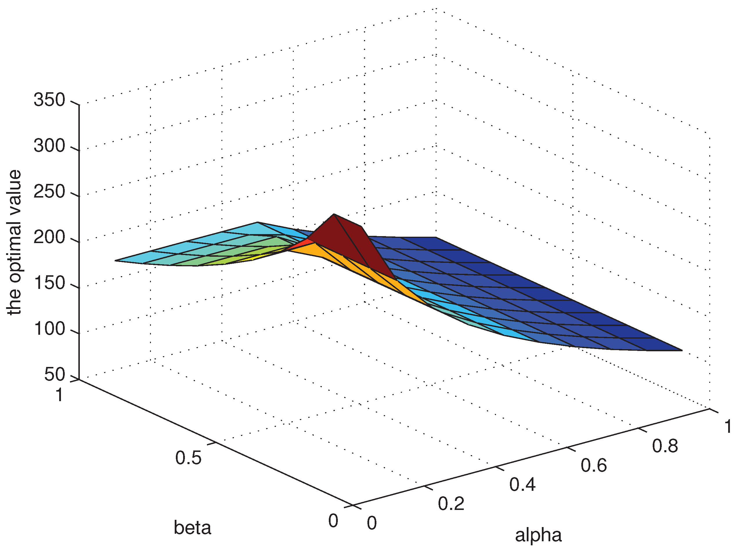
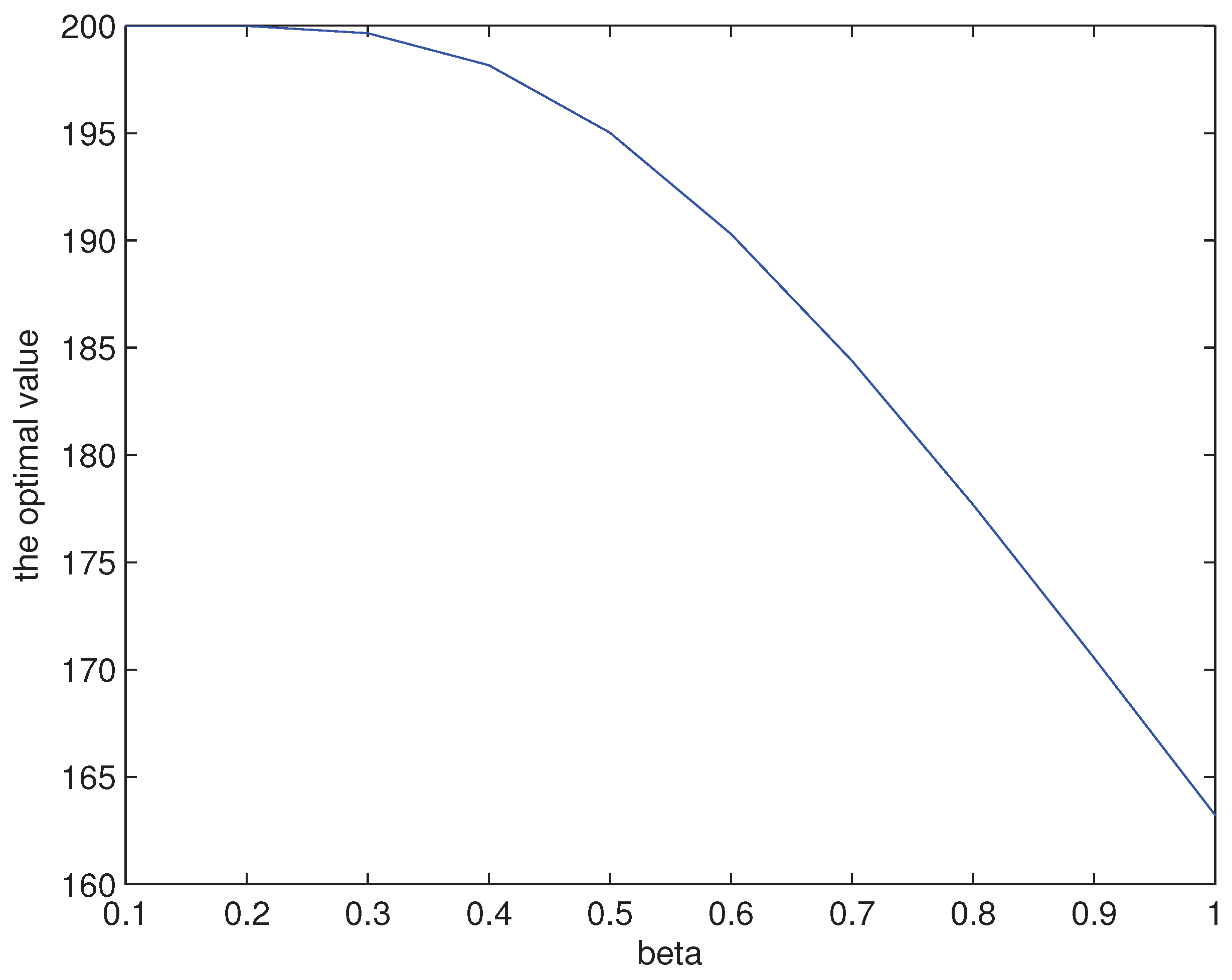
According to Lemma 1, Problem (3) is equivalent to
inf f c , d H 0 1 α 0 α [ S X 1 ( λ ) f c , d ( S X 1 ( λ ) ) ] d λ + 1 + θ β 0 β f c , d ( S X 1 ( x ) ) d x = inf ( c , d ) D ( 1 α 0 α [ S X 1 ( λ ) [ ( S X 1 ( λ ) c ) + ( S X 1 ( λ ) d ) + ] ] d λ + 1 + θ β 0 β [ ( S X 1 ( x ) c ) + ( S X 1 ( x ) d ) + ] d x ) .
Problem (13) is reduced by Problem (2) by shrinking the probability measure set M 1 to the singleton { Φ } with Φ = δ α with α [ 0 , 1 ] fixed. Here, δ α ( { α } ) = 1 .
We take the infimum given by (13) as the bivariate function of ( α , β ) , and numerically investigate how sensitively the value of ( α , β ) will affect our optimal value. The corresponding numerical results are given by Figure 1 below. It seems that significant differences in the size of optimal value can be obtained depending on the value of ( α , β ) . It also seems that the optimal value increases as α and β approaches 0.
(ii)
Consider the following optimization problem,
inf f H 0 1 1 α 0 α [ S X 1 ( λ ) f ( S X 1 ( λ ) ) ] d λ d Φ ( α ) + 1 + θ β 0 β f ( S X 1 ( x ) ) d x = inf ( c , d ) D ( 0 1 1 α 0 α [ S X 1 ( λ ) [ ( S X 1 ( λ ) c ) + ( S X 1 ( λ ) d ) + ] ] d λ d Φ ( α ) + 1 + θ β 0 β [ ( S X 1 ( x ) c ) + ( S X 1 ( x ) d ) + ] d x ) ,
with d Φ ( α ) = 1 d α , α [ 0 , 1 ] . Problem (14) is another particular case of Problem (2). In fact, Problem (14) is reduced by Problem (2) by shrinking the probability measure set M 1 to the singleton { Φ } .
We take the infimum given by (14) as the function of β, and numerically investigate how sensitively the value of β will affect our optimal value. The corresponding numerical results are given by Figure 2 below. It can be seen that the optimal value decreases as the value of β increases.

5. Concluding Remarks

In this paper, we study the optimal reinsurance problem under the general law-invariant convex risk measure and the TVaR premium principle. Cheung, et al. [19] considered the analogous problem with the premium being calculated via the expected premium principle. It is worth mentioning that the TVaR premium principle we considered is an extension of the expected premium principle. However, since the general law-invariant risk measures considered in this paper (and Cheung, et al. [19]) are a class of very general risk measures, it is not easy to make further extensions for the premium principle. The optimal reinsurance strategy which minimizes the insurer’s risk measure of its total loss is characterized. Our results show that the optimal reinsurance strategy is of the multi-layer form, which is also an extended version of that in Cheung, et al. [19].

Acknowledgments

Supported in part by the National Natural Science Foundation of China (Nos., 11401498, 11661074), Natural Science Foundation of Fujian Province (No. 2015J05003) and the Fundamental Research Funds for the Central Universities of China (No. 20720140525), Zhejiang Provincial Natural Science Foundation of China (No. LY16A010001), Zhejiang Provincial Key Research Base for Humanities and Social Sciences grant (statistics), and Zhejiang Educational Committee (No. 1020KZ0413455).

Author Contributions

These authors contributed equally to the paper.

Conflicts of Interest

The authors declare no conflict of interest.

References

  1. K. Borch. “An attempt to determine the optimum amount of stop loss reinsurance.” In Proceedings of the Transactions of the 16th International Congress of Actuaries, Brussels, Belgium, 15–22 June 1960; pp. 597–610.
  2. M. Kaluszka. “Optimal reinsurance under mean-variance premium principles.” Insur. Math. Econ. 28 (2001): 61–67. [Google Scholar] [CrossRef]
  3. R. Kaas, M. Goovaerts, J. Dhaene, and M. Denuit. Modern Actuarial Risk Theory. Boston, MA, USA: Kluwer Academic Publishers, 2001. [Google Scholar]
  4. J. Cai, Y. Fang, Z. Li, and G. Willmot. “Optimal reciprocal reinsurance treaties under the joint survival probability and the joint profitable probability.” J. Risk Insur. 80 (2013): 145–168. [Google Scholar] [CrossRef]
  5. Y. Chi. “Reinsurance arrangements minimizing the risk-adjusted value of an insurer’s liability.” Insur. Math. Econ. 42 (2012): 529–557. [Google Scholar] [CrossRef]
  6. K.C. Cheung, W.F. Chong, and S.C.P. Yam. “The optimal insurance under disappointment theories.” Insur. Math. Econ. 64 (2015): 77–90. [Google Scholar] [CrossRef]
  7. M. Kaluszka. “An extension of Arrow’s result on optimality of a stop-loss contract.” Insur. Math. Econ. 35 (2004): 527–536. [Google Scholar] [CrossRef]
  8. M. Kaluszka. “Optimal reinsurance under convex principles of premium calculation.” Insur. Math. Econ. 36 (2005): 375–398. [Google Scholar] [CrossRef]
  9. L. Gajek, and D. Zagrodny. “Optimal reinsurance under general risk measures.” Insur. Math. Econ. 34 (2004): 227–240. [Google Scholar] [CrossRef]
  10. S.D. Promislow, and V.R. Young. “Unifying framework for optimal insurance.” Insur. Math. Econ. 36 (2005): 347–364. [Google Scholar] [CrossRef]
  11. J. Cai, K.S. Tan, C.G. Weng, and Y. Zhang. “Optimal reinsurance under VaR and CTE risk measures.” Insur. Math. Econ. 43 (2008): 185–196. [Google Scholar] [CrossRef]
  12. A. Balbás, B. Balbás, and A. Heras. “Optimal reinsurance with general risk measures.” Insur. Math. Econ. 44 (2009): 374–384. [Google Scholar] [CrossRef]
  13. K.C. Cheung. “Optimal reinsurance revisited-a geometric approach.” ASTIN Bull. 40 (2010): 221–239. [Google Scholar] [CrossRef]
  14. Y. Chi, and C. Weng. “Optimal reinsurance subject to Vajda condition.” Insur. Math. Econ. 53 (2013): 179–189. [Google Scholar] [CrossRef]
  15. Y. Chi, and K.S. Tan. “Optimal reinsurance under VaR and CVaR risk measures: A simplified approach.” ASTIN Bull. 41 (2011): 487–509. [Google Scholar]
  16. K.C. Cheung, and A. Lo. “Characterizations of optimal reinsurance treaties: A cost-benefit approach.” Scand. Actuar. J., 2015. [Google Scholar] [CrossRef]
  17. K.C. Cheung, K.C.J. Sung, S.C.P. Yam, and S.P. Yung. “Optimal reinsurance under general law-invariant risk measures.” Scand. Actuar. J. 2014 (2014): 72–91. [Google Scholar] [CrossRef]
  18. Z. Lu, L. Liu, Q. Shen, and L. Li. “Optimal reinsurance under VaR and CTE risk measures when ceded loss function is concave.” Commun. Stat. Theory Methods 43 (2014): 3223–3247. [Google Scholar] [CrossRef]
  19. H. Assa. “On optimal reinsurance policy with distortion risk measures and premiums.” Insur. Math. Econ. 61 (2015): 70–75. [Google Scholar] [CrossRef]
  20. Y.T. Zheng, and W. Cui. “Optimal reinsurance with premium constraint under distortion risk measures.” Insur. Math. Econ. 59 (2014): 109–120. [Google Scholar] [CrossRef]
  21. W. Cui, J.P. Yang, and L. Wu. “Optimal reinsurance minimizing the distortion risk measure under general reinsurance premium principles.” Insur. Math. Econ. 53 (2013): 74–85. [Google Scholar] [CrossRef]
  22. Y. Zhu, Y. Chi, and C. Weng. “Multivariate reinsurance designs for minimizing an insurer’s capital requirement.” Insur. Math. Econ. 59 (2014): 144–155. [Google Scholar] [CrossRef]
  23. Y. Chi, and K.S. Tan. “Optimal reinsurance with general premium principles.” Insur. Math. Econ. 52 (2013): 180–189. [Google Scholar] [CrossRef]
  24. X. Hu, H. Yang, and L. Zhang. “Optimal retention for a stop-loss reinsurance with incomplete information.” Insur. Math. Econ. 65 (2015): 15–21. [Google Scholar] [CrossRef]
  25. J. Cai, and K.S. Tan. “Optimal retention for a stop-loss reinsurance under the VaR and CTE risk measures.” ASTIN Bull. 37 (2007): 93–112. [Google Scholar] [CrossRef]
  26. A. Asimit, A. Badescu, and T. Verdonck. “Optimal risk transfer under quantile-based risk measurers.” Insur. Math. Econ. 53 (2013): 252–265. [Google Scholar] [CrossRef]
  27. K.J. Arrow. “Optimal insurance and generalized deductibles.” Scand. Actuar. J. 1 (1974): 1–42. [Google Scholar] [CrossRef]
  28. C.Y. Zhou, W.F. Wu, and C.F. Wu. “Optimal insurance in the presence of insurer’s loss limit.” Insur. Math. Econ. 46 (2010): 300–307. [Google Scholar] [CrossRef]
  29. K.C. Cheung, F. Liu, and S.C.P. Yam. “Average Value-at-Risk minimizing reinsurance under Wang’s premium principle with constraints.” ASTIN Bull. 42 (2012): 575–600. [Google Scholar]
  30. K. Tan, and C. Weng. “Enhancing insurer value using reinsurance and Value-at-Risk criterion.” Geneva Risk Insur. Rev. 37 (2012): 109–140. [Google Scholar] [CrossRef]
  31. V.R. Young. “Premium principles.” Encycl. Actuar. Sci. 3 (2004): 132–1331. [Google Scholar]
  32. H. Föllmer, and A. Schied. StochastiC Finance: An Introduction in Discrete Time, 4th ed. Berlin, Germany: Walter de Gruyter, 2016. [Google Scholar]
  33. J. Belles-Sampera, M. Guillén, and M. Santolino. “Beyond Value-at-Risk: GlueVaR Distortion Risk Measures.” Risk Anal. 34 (2014): 121–134. [Google Scholar] [CrossRef] [PubMed]
Figure 1. The horizontal axis represents β, the vertical axis represents α, the lateral axis represents the optimal value given by (13). The Greek θ is set to be 0.1. The distribution of X is exponential: S X ( x ) = e 1 100 x .
Risks 04 00050 g001
Figure 2. The horizontal axis represents β, the vertical axis represents the optimal value given by (14). The Greek θ is set to be 0.1. The distribution of X is exponential: S X ( x ) = e 1 100 x .
Risks 04 00050 g002

