Change Point Detection and Estimation of the Two-Sided Jumps of Asset Returns Using a Modified Kalman Filter

Abstract

In the first part of the paper, the positive and negative jumps of NASDAQ daily (log-) returns and three of its stocks are estimated based on the methodology presented by Theodosiadou et al. 2016, where jumps are assumed to be hidden random variables. For that reason, the use of stochastic state space models in discrete time is adopted. The daily return is expressed as the difference between the two-sided jumps under noise inclusion, and the recursive Kalman filter algorithm is used in order to estimate them. Since the estimated jumps have to be non-negative, the associated pdf truncation method, according to the non-negativity constraints, is applied. In order to overcome the resulting underestimation of the empirical time series, a scaling procedure follows the stage of truncation. In the second part of the paper, a nonparametric change point analysis concerning the (variance–) covariance is applied to the NASDAQ return time series, as well as to the estimated bivariate jump time series derived after the scaling procedure and to each jump component separately. A similar change point analysis is applied to the three other stocks of the NASDAQ index.

1. Introduction

It has been proven empirically that asset returns do not only evolve continuously over time, as proposed in [1], but also include jumps. Cox and Ross in [2] and Merton in [3] argue that the theories developed for asset pricing based on the continuous evolution of returns have to be modified in order to incorporate exposure to the jump risk. Afterward, there were plenty of papers adopting models with jumps in order to describe the empirical data of asset returns (see for example [4,5,6]). Furthermore, in [7] jumps appearing in small or high frequencies were examined. Among the studies concerning the detection of jumps in high frequency financial data, Barndorff-Nielsen and Shephard ([8,9]) contributed significantly to the literature. In [10] jumps in daily returns are considered to be hidden random variables (RVs) and they are divided into two categories: positive (upward) jumps due to the arrival of positive news in the market and negative (downward) jumps due to the arrival of negative news in the market. In [11] a sensitivity analysis of the model proposed in [10] was developed, whereas in [12] the adjustment of that model to real data was examined.

The first target in the present paper is to estimate the positive and negative jumps in the daily asset (log-) return time series. Due to the fact that the two sided jumps are thought of as hidden RVs, i.e., not observable RVs, the use of a time-homogeneous stochastic-state space model is adopted, as presented in [13]. Time series analysis based on state space methods can be found for example in [14,15,16,17]. The estimations of the hidden jumps are provided by the recursive Kalman filter algorithm ([18]). However, due to the fact that the daily return is expressed as the difference between the positive and negative jump under noise inclusion ([13]), the estimated jumps have to be non-negative for every t. For that purpose, the method of the common (bivariate) pdf truncation of the jumps is used and the mean values derived through the truncation are considered to be the corrected estimations of the jumps. Finally, in order to overcome the underestimation of the empirical time series due to the truncation, an appropriate scaling procedure follows.

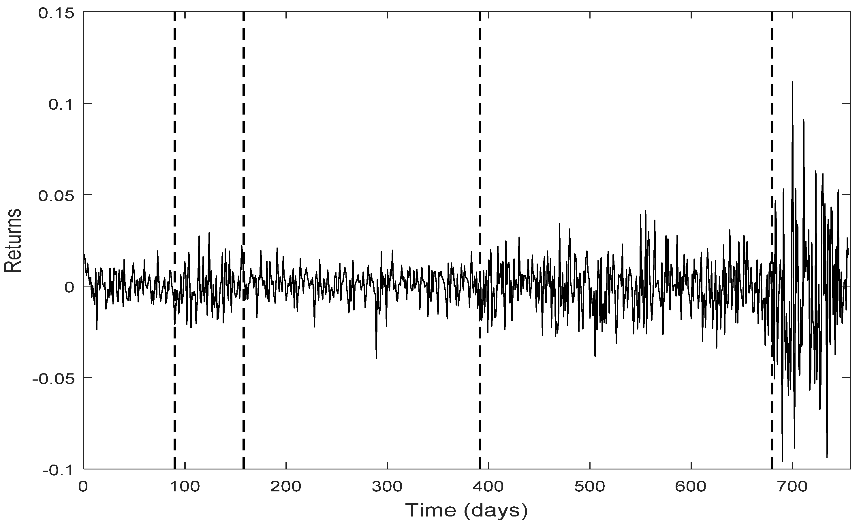
The second target in the present paper is to apply a change point analysis concerning the variance–covariance of the data, as well the estimated bivariate jump series derived via the state space model proposed in [13] and each jump component separately. This analysis allows us to detect similarities and differences between the estimated structural breaks in the aforementioned time series.

The data used in the paper in order to analyze the targets stated above and get the relevant results concern the NASDAQ time series during the three-year period of 2006–2008 (755 observations) and three of its stocks, namely Google, Intel and Microsoft (historical prices were derived from finance.yahoo.com). This data sample is a strongly declining period for the NASDAQ index and was used for analysis in [10,11,12,13].

The paper is organized as follows:

In Section 2, the state space model proposed in [13] and the estimation of the NASDAQ index via the aforementioned model are briefly presented. In Section 3.1, the change points regarding the NASDAQ time series and the estimated jumps are illustrated, while in Section 3.2 a similar presentation is exhibited for the NASDAQ stocks. Finally, in Section 4, conclusions and remarks concerning the structural breaks of the time series examined are provided.

2. The Model

In [13] a linear Markovian state space model was established for the estimation of the two-sided jumps of the daily asset (log-) returns. In this model the states, which are the hidden RVs of the model, represent the daily positive and negative return jumps. If we denote the following:

• ${\mathrm{X}}_t$: the positive (upward) jump of NASDAQ return at time t,
• ${\mathrm{Y}}_t$: the negative (downward) jump of NASDAQ return at time t,
• ${\mathrm{R}}_t$: the return at time t, 1

the state equation of the proposed model becomes

$$\begin{array}{l}{\mathrm{X}}_t={\mathrm{g}}_{11}{\mathrm{X}}_{t-1}+{\mathrm{g}}_{12}{\mathrm{Y}}_{t-1}+{\mathrm{w}}_{1,t-1}\\ {\mathrm{Y}}_t={\mathrm{g}}_{21}{\mathrm{X}}_{t-1}+{\mathrm{g}}_{22}{\mathrm{Y}}_{t-1}+{\mathrm{w}}_{2,t-1}\end{array}\},t=1,2,\dots$$

(1)

or in matrix form

$${\mathbf{z}}_t=G{\mathbf{z}}_{t-1}+w_{t-1},t=1,2,\dots ,$$

where

$${\mathbf{z}}_t=\left(\begin{array}{c}{\mathrm{X}}_t\\ Y_t\end{array}\right),G=\left(\begin{array}{cc}{g}_{11}& g_{12}\\ g_{21}& g_{22}\end{array}\right),w_{t-1}=\left(\begin{array}{c}{w}_{1,t-1}\\ w_{2,t-1}\end{array}\right).$$

The asset return measurement equation of the model is of the form

$${\mathrm{R}}_t={\mathrm{X}}_t-{\mathrm{Y}}_t+{\mathrm{e}}_t,t=1,2,\dots$$

(2)

or in matrix form

$${\mathrm{R}}_t=H{\mathbf{z}}_t+{\mathrm{e}}_t,t=1,2,\dots$$

where H = (1,−1). Moreover, we assume that $w_t$ and ${\mathrm{e}}_t$ are normal white noises with variance–covariance matrices Q and V respectively, i.e.,

$$w_t~\mathrm{N}\left(0,Q=\left(\begin{array}{cc}{\mathrm{s}}_{\mathrm{x}}^2& 0\\ 0& {\mathrm{s}}_{\mathrm{y}}^2\end{array}\right)\right),{\mathrm{e}}_{\mathrm{t}}~\mathrm{N}(0,\mathrm{V})$$

and

$$\mathrm{E}\left[w_{\mathrm{k}}{w}_{\mathrm{j}}^{\mathrm{T}}\right]=Q{\mathsf{\delta }}_{\mathrm{k},\mathrm{j}},{\mathrm{E}[\mathrm{e}}_{\mathrm{k}}{\mathrm{e}}_{\mathrm{j}}^{\mathrm{T}}{]=\mathrm{V}\mathsf{\delta }}_{\mathrm{k},\mathrm{j}},{\mathrm{E}[\mathrm{e}}_{\mathrm{k}}{w}_{\mathrm{j}}^{\mathrm{T}}]=0.$$

Notice that model (1)–(2) is time-homogeneous, in the sense that the matrices G, H, Q and V are time-invariant.

Our target is to estimate the hidden jumps Χ_t and Y_t by using model (1)–(2). Given that the return R_t is expressed as the difference between the positive and negative jump at time t under noise inclusion, the estimated jumps Χ_t and Y_t that satisfy relation (2) must be non-negative, i.e., Χ_t, Y_t ≥ 0 for every t = 1,2,... .

The estimation of the hidden states Χ_t and Y_t in model (1)–(2) is attained by first using (stage 1) the recursive algorithm of the standard Kalman filter, which provides the optimal linear estimators, that is, the minimum mean squared error estimators. The Kalman filter proceeds in two steps; in the first step (prediction step), the hidden state z_t as well as the related error variance–covariance matrix are predicted, using all the information till time t−1. At the second step (updating step), the estimation of z_t is updated-corrected by taking into account the measurement at time t.

Now, let ${\hat{\mathrm{z}}}_t^{-}$, ${\hat{\mathrm{z}}}_t^{+}$ be the a priori and a posteriori estimation of some state z_t respectively, and $P_t^{-}$, $P_t^{+}$ the variance–covariance matrices of the a priori and a posteriori error estimations of z_t, respectively, i.e.,

$$P_t^{-}=\mathrm{E}\left[\left(z_t-{\widehat{z}}_t^{-}\right){\left(z_t-{\widehat{z}}_t^{-}\right)}^{\mathrm{T}}\right]\mathrm{and}{P}_t^{+}=\mathrm{E}\left[\left(z_t-{\widehat{z}}_t^{+}\right){\left(z_t-{\widehat{z}}_t^{+}\right)}^{\mathrm{T}}\right].$$

Then, the recursive equations of Kalman filtering in discrete time are given in

Table 1. Equations of the discrete Kalman filter.

A priori estimator of the state zt	${\hat{\mathbf{z}}}_{\mathit{t}}^{-}{=\mathbf{G}\hat{\mathbf{z}}}_{\mathit{t}-1}^{+},$
Variance–covariance matrix of the a priori error estimation	$P_t^{-}=G{P}_{t-1}^{+}{G}^{\mathrm{T}}+Q$
Prediction error	${\mathrm{u}}_t={\mathrm{R}}_t-H{\widehat{z}}_t^{-}$
Variance of the prediction error	${\mathsf{\Omega }}_t=H{P}_t^{-}{H}^{\mathrm{T}}+\mathrm{V}$
Kalman gain matrix	$K_t=P_t^{-}{H}^{\mathrm{T}}{\left(H{P}_t^{-}{H}^{\mathrm{T}}+\mathrm{V}\right)}^{-1}$
A posteriori estimator of the state zt	$z_t^{+}={\widehat{z}}_t^{-}+K_t\left({\mathrm{R}}_t-H{\widehat{z}}_t^{-}\right),$
Variance– covariance matrix of the a posteriori error estimation	$P_t^{+}=\left(I-K_{t}H\right)P_t^{-}$

.

Now in order to initialize the filter, since there are no measurements at time t = 0, we assume that

$${\widehat{z}}_0^{+}=\mathrm{E}(z_0)\mathrm{and}{P}_0^{+}=\mathrm{E}\left[\left(z_0-{\widehat{z}}_0^{+}\right){\left(z_0-{\widehat{z}}_0^{+}\right)}^{\mathrm{T}}\right]$$

Note that before running the Kalman filter algorithm in order to get the estimates of the hidden states z_t, the unknown parameters of model (1)–(2) have to be estimated, i.e., the transition matrix G and the variances s_x ², s_y ² and V. For that purpose, the method of maximum likelihood estimation is used (MLE). Since the RV R_t conditional on R_t−1 follows in the standard Kalman filter procedure a normal distribution, i.e., ${\mathrm{R}}_{t/t-1}~\mathrm{N}(H{\widehat{z}}_t^{-},{\mathsf{\Omega }}_t)$, the log-likelihood function (LogL) has the form

$$\mathit{LogL}\left({\mathrm{R}}_1,...,{\mathrm{R}}_n\right)=-\frac{n}{2}\mathit{log}\left(2\pi \right)-\frac{1}{2}{\displaystyle \sum _{t=1}^n\left(\mathit{log}\left(\left|{\mathsf{\Omega }}_t\right|\right)+{\mathrm{u}}_t^{\mathrm{T}}{\mathsf{\Omega }}_t^{-1}{\mathrm{u}}_t\right)},n=755.$$

In the case of NASDAQ index using the data from the period 2006-2008, we get the estimates ([13])

$$G=\left(\begin{array}{cc}0.3883& 0.5512\\ 0.5163& 0.4232\end{array}\right),Q=\left(\begin{array}{cc}9.4658\times {10}^{-5}& 0\\ 0& 9.4658\times {10}^{-5}\end{array}\right)\mathrm{and}\mathrm{V}=9.4658\times {10}^{-5}.$$

In [13] the positive and negative jumps of the daily NASDAQ returns during the 3-year period 2006–2008 are estimated by using the Kalman filter recursive algorithm based on model (1)–(2) (stage 1). However, the resulting estimated jumps do not satisfy the non-negativity condition for every t. Therefore, the initial estimations of the jumps derived at stage 1 are corrected through an additional two-stage procedure ([13]), first by truncating the bivariate common distribution of the positive and negative jumps (stage 2). Through this truncation, new (non-negative) estimations of the state vectors are derived, which are considered to be the mean values of the truncated distributions.

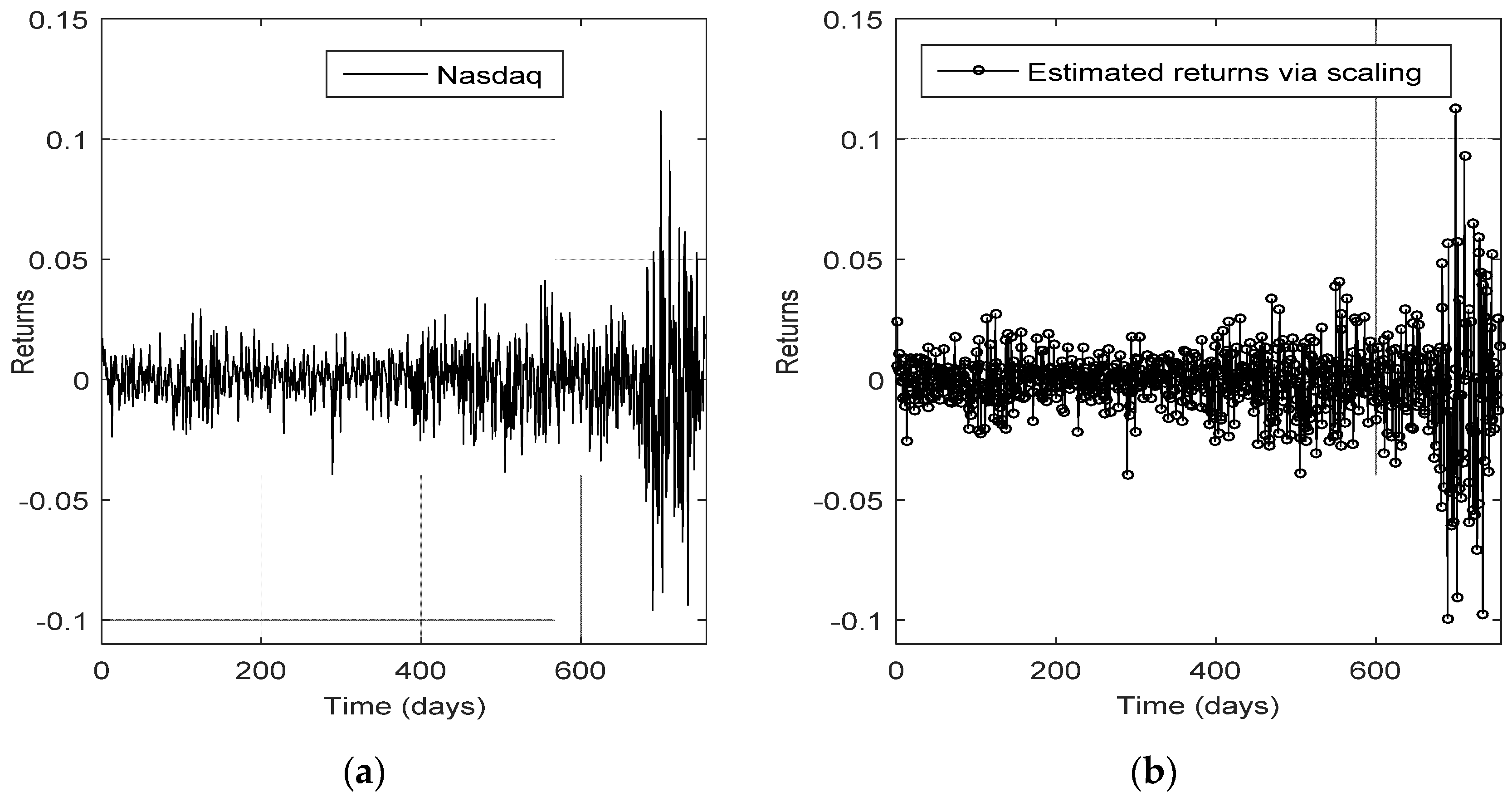
Next, comparing the resulting return time series based on the pdf truncation method with the empirical returns of the NASDAQ index, it is found that the estimated time series underestimates the empirical returns for every t (Figure 3 in [13]).For that reason, a new correction procedure to the last estimations is applied (stage 3), where the estimated jumps resulted through the pdf truncation method are rescaled by a scaling factor evaluated via linear regression.

Notice that the 3-stage estimation process presented above goes beyond the linear Kalman filtering process (applied at stage 1), because of the additional estimation stages 2 and 3. So the resulting model constitutes an extension-modification of the Kalman filter.

The very satisfactory adjustment of the estimated NASDAQ return time series derived by means of the aforementioned procedure can be seen in Figure 1, in which the graphs of the empirical and the estimated returns almost coincide with each other.

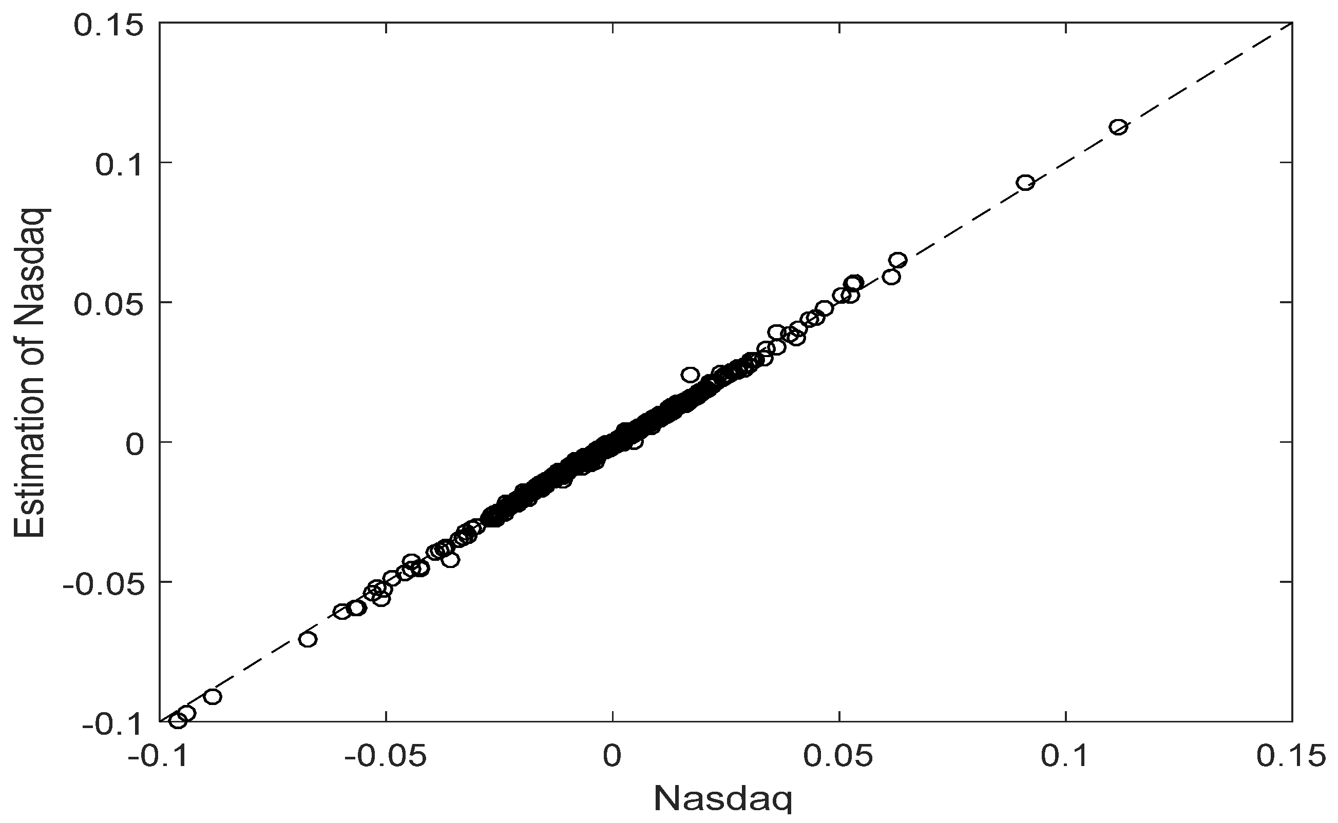
Alternatively, the associated Q-Q (Quantile-Quantile) plot verifying the very satisfactory adjustment can be seen in the following Figure 2.

The result of Kolmogorov-Smirnov goodness of fit test and the small value of the mean squared error (MSE) confirm the above conclusion, as

K.S. stat = 0.0609 with associated p-value = 0.1169, MSE = 1.41 × 10⁻⁶.

3. Change Point Detection for the Empirical and the Estimated Time Series

3.1. Change Point Detection for NASDAQ

In this section, we proceed to a change point analysis in order to detect the change points in the (variance–)covariance structure of the NASDAQ return time series and the estimated bivariate jump time series via the scaling procedure. Furthermore, we check for the change points of the two marginals, i.e., the estimated positive and negative jumps separately. The change point detection indicates a structural break in the time series under study.

In order to detect change points in the (variance–) covariance structure of a d-dimensional time series ${\mathbf{a}}_1,\dots ,{\mathbf{a}}_n$, where ${\mathbf{a}}_t=\left(a_{t,1},\dots ,a_{t,d}\right)$, $d\in N,$ we apply below a nonparametric test based on [19]. The associated test statistic is given by,

$${\mathrm{A}}_{\mathrm{n}}={\mathit{max}}_{1\le t\le n}{\displaystyle \sum _{t=1}^{\mathrm{n}}{\tilde{\mathrm{S}}}_t^{\mathrm{T}}}\tilde{\Lambda }{\tilde{\mathrm{S}}}_t,$$

where

$${\tilde{S}}_t=\frac{1}{\sqrt{n}}\left({\displaystyle \sum _{t=1}^{\mathrm{k}}\mathit{vech}\left[{\tilde{\mathsf{\alpha }}}_t{\tilde{\mathsf{\alpha }}}_t^{{T}}\right]}-\frac{k}{n}{\displaystyle \sum _{t=1}^{\mathrm{k}}\mathit{vech}\left[{\tilde{\mathsf{\alpha }}}_t{\tilde{\mathsf{\alpha }}}_t^{\mathrm{T}}\right]}\right),t=1,...,n$$

and ${\tilde{\mathbf{a}}}_i={\mathbf{a}}_t-{\overline{\mathbf{a}}}_n.$ 2 The matrix $\tilde{\mathit{\Lambda }}$ represents a kernel-based estimator of the long-run covariance. The asymptotic distribution of the test statistic is

$$su{p}_{0\le t\le 1}{{\displaystyle \sum }}_{j=1}^{d\left(d+1\right)/2}{B}_j^2\left(t\right)$$

where $\left(B_j\left(t\right):t\in \left[0,1\right]\right),1\le j\le d\left(d+1\right)/2)$ are independent Brownian bridges. We calculate critical values at a significance level of 5%, as given in [20]. Critical values are presented in

Table 2. Critical values.

Sample Size	One Dimension	Two Dimensions
200	0.6194	2.2629
500	0.6492	2.3807
750	0.6646	2.4833

for N = 3000 simulations.

As we are looking for the case of multiple change points, we apply a binary segmentation algorithm to the statistic. Notice that we have to exclude the first change point of the estimated time series, say for $t\in \left[1,15\right]$, due to the high uncertainty of the change point detection attained at the beginning of the time series.

Based on the test described in [19], we detect four change points at t = 90, 158, 391, 680 in the (empirical) NASDAQ time series. The results are illustrated in

Table 3. Change points for NASDAQ index with the corresponding test statistic value.

t (in Days)	Date	An
90	9/5/2006	1.5127
158	15/8/2006	0.6252
391	20/7/2007	6.6824
680	14/9/2008	9.8852

and Figure 3 below.

Using the same methodology as for the NASDAQ index, we detect two change points at t = 391, 673 for the estimated bivariate jump series, which are almost the same as the two clear change points in the (univariate) NASDAQ time series.

Table 4. Change points in the estimated bivariate jump time series for NASDAQ index with the corresponding test statistic value.

t (in Days)	Date	An
391	20/7/2007	7.3045
673	2/9/2008	10.1606

and Figure 4 exhibit the relevant results.

Finally, as in the previous cases, we show in

Table 5. Change points in the estimated positive jump time series of NASDAQ index with the corresponding test statistic value.

t (in Days)	Date	An
114	13/6/2006	0.748
158	15/8/2006	1.371
399	1/8/2007	4.3989
682	15/9/2008	5.9239

and

Table 6. Change points in the estimated negative jump time series of NASDAQ index with the corresponding test statistic value.

t (in Days)	Date	An
391	20/7/2007	5.1768
673	2/9/2008	8.8262

and in Figure 5 the change points in the two estimated marginal time series, i.e., the time series of the positive and the negative jumps.

Interestingly, it can be concluded from Figure 5 that the sets of the change points in each jump component do not coincide with each other. On the other hand, the change points of the bivariate jump time series coincide with the notable change points (i.e., with those that have the highest value of test statistic) of the two jump components. Furthermore, the change points of the NASDAQ index are almost the same with the change points of the positive jumps. We notice that change points in different time series which appear to differ slightly (concerning the estimated time) probably indicate the same time point.

3.2. Change Point Detection in NASDAQ Stocks

A similar change point analysis, as the one presented in Section 3.1, is shown below for Google, Intel and Microsoft stocks during the 3-year period of 2006–2008 in order to see if the above conclusions concerning changes in the (variance–) covariance structure also hold for other return time series.

First, we have to ‘reveal’ the hidden positive and negative jumps for each stock based on the proposed model (1)–(2). For that purpose, we estimate the parameters of the model (1)–(2) via the MLE method for each stock. Then, we estimate the bivariate jump time series using the Kalman filter accompanied by the truncation and scaling procedure.

Table 7. Estimation of the transition matrix G of model (1)–(2).

Stock	g11	g12	g21	g22
Google	0.2959	0.4396	0.1466	0.2360
Intel	8.2780	−8.9901	8.6001	−9.2657
Microsoft	6.3131	−6.9034	6.5867	−7.1254

and

Table 8. Estimation of the variances of model (1)–(2).

Stock	sx2	sy2	V
Google	3.9009 × 10−5	1.7301 × 10−4	4.0115 × 10−4
Intel	2.4050 × 10−8	1.0696× 10−4	3.8919× 10−4
Microsoft	1.3176 × 10−8	1.3380 × 10−4	2.5682× 10−4

below illustrate the estimated parameters for each stock.

Using the methodology proposed in [19], as in the case of NASDAQ index, we are going to detect the change points concerning the variance–covariance in the time series of each stock. Firstly, we estimate the respective bivariate jump time series based on model (1)–(2), and each jump component separately. The relevant change point analysis for Google is presented below.

It can be seen by

Table 9. Change points for Google with the corresponding test statistic value.

t (in Days)	Date	An
40	27/2/2006	0.6764
92	11/5/2006	3.3164
295	5/3/2007	0.8226
443	3/10/2007	0.7781
505	2/1/2008	5.1378
682	15/9/2008	1.3997

,

Table 10. Change points in the estimated bivariate jump time series for Google with the corresponding test statistic value.

t (in Days)	Date	An
92	11/5/2006	3.253
505	2/1/2008	6.9468
682	15/9/2008	2.4223

,

Table 11. Change points in the estimated positive jump time series of Google with the corresponding test statistic value.

t (in Days)	Date	An
47	8/3/2006	2.3257
92	11/5/2006	0.8249
464	1/11/2007	1.15
513	14/1/2008	4.5327
682	15/9/2006	1.5225

and

Table 12. Change points in the estimated negative jump time series of Google with the corresponding test statistic value.

t (in Days)	Date	An
58	23/5/2006	0.7286
109	6/6/2006	1.4899
296	6/3/2007	0.77
466	5/11/2007	1.5561
518	22/1/2008	3.6611
579	18/4/2008	0.6628
638	14/7/2008	0.838
690	25/9/2008	0.7078

and Figure 6 that no one of the four sets of change points (i.e., the empirical Google, the bivariate estimated time series, the positive jumps and the negative jumps), coincides with any one of the other three. Once more, notice that change points which differ slightly (for example 505, 513, 518 in Table 9, Table 10, Table 11 and Table 12) may be considered to indicate in fact the same time. The change points for the empirical Google returns and the estimated bivariate time series are also change points for the positive or the negative jumps. The cardinality of the set of change points for the bivariate time series is the smallest one.

In the sequel, the results for Intel are demonstrated.

It can be easily seen by the results in

Table 13. Change points for Intel with the corresponding test statistic value.

t (in Days)	Date	An
503	28/12/2007	6.8067
527	4/2/2008	1.2989
689	24/9/2008	3.2335

,

Table 14. Change points in the estimated bivariate jump time series of Intel with the corresponding test statistic value.

t (in Days)	Date	An
451	15/10/2007	2.4258
682	15/9/2008	8.9164

,

Table 15. Change points for the estimated positive jumps of Intel with the corresponding test statistic value.

t (in Days)	Date	An
122	23/6/2006	2.1747
157	14/8/2006	1.1001
384	11/7/2007	3.1743
683	16/9/2008	6.814

and

Table 16. Change points for the estimated negative jumps of Intel with the corresponding test statistic value.

t (in Days)	Date	An
452	16/10/2007	3.4116
506	31/1/2008	1.9679
522	28/1/2008	0.6362
684	17/9/2008	6.5641

and Figure 7 that the change points in Intel and the estimated bivariate jump time series are also change points of the two jump components and they generally appear to have the highest test statistic value.

Finally, the results for the Microsoft stock are shown below.

The results derived for empirical Microsoft returns, the estimated bivariate jump time series and the marginal univariate jump components, presented in

Table 17. Change points for Microsoft with the corresponding test statistic value.

t (in Days)	Date	An
162	21/8/2006	0.6632
257	8/1/2007	1.385
451	15/10/2007	2.3171
637	11/7/2008	5.9491
690	25/9/2008	1.1384

,

Table 18. Change points in the estimated bivariate jump time series of Microsoft with the corresponding test statistic value.

t (in Days)	Date	An
451	15/10/2007	3.3099
678	9/9/2008	6.7154

,

Table 19. Change points for the estimated positive jumps of Microsoft with the corresponding test statistic value.

t (in Days)	Date	An
82	27/4/2006	0.7834
147	31/7/2006	0.7879
258	9/1/2007	1.0501
454	18/10/2007	1.2919
683	16/9/2008	3.6418
713	28/10/2008	0.6252

and

Table 20. Change points for the estimated negative jumps of Microsoft with the corresponding test statistic value.

t (in Days)	Date	An
82	27/4/2006	0.7626
147	31/7/2006	0.8131
259	10/1/2007	1.0131
455	19/10/2007	1.3885
692	16/9/2008	3.6418
713	28/10/2008	0.8441

and Figure 8, are similar to the results derived for Intel, presented just after Figure 6. Here the change points for the positive and negative components are almost the same.

Apart from some special features exhibited in the change point analysis of the NASDAQ index, the three aforementioned stocks and their jump components, some general conclusions concerning change point detection can be derived according to the results demonstrated in the related tables and figures; these conclusions are presented in the next section.

4. Conclusions

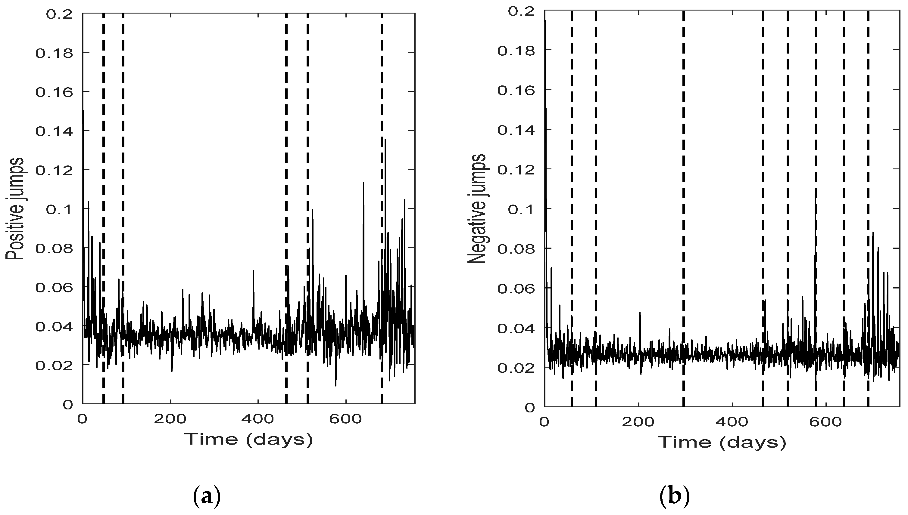
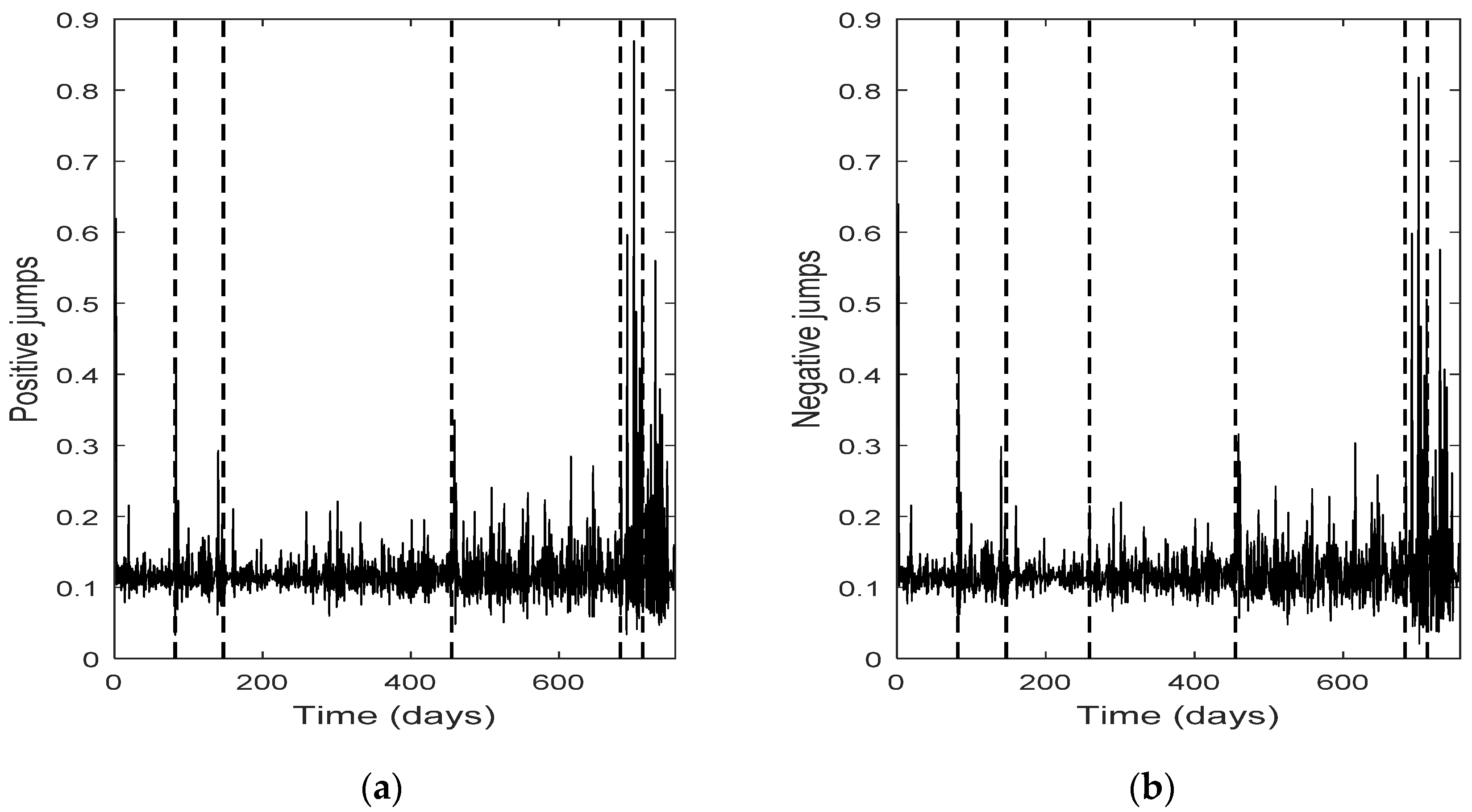
In this paper, the positive and negative jumps of NASDAQ index and four of its stocks are estimated in order to detect the (variance–) covariance structural breaks (change points) in the related time series. The estimation of the positive and negative jumps is achieved by means of the methodology presented in [13], i.e., using Kalman filtering, accompanied by truncation and scaling of the resulting jump distributions.

The change point detection in the final positive and negative jumps time series show that the change points of the two separate jump components usually do not coincide, while the intersection of the two corresponding change point sets is not empty; it consists of the change points with the highest test statistic value (A_n). Each marginal jump time series includes change points detected in the bivariate time series and the time series of the empirical returns, and probably other points too. The cardinality of the set of change points for the bivariate time series is, in all four cases, the smallest one.

Furthermore, the set of the change points for the bivariate jump time series consists of those change points of the univariate jump components which have the highest values of the test statistic. In other words, the higher the value of the test statistic for a change point detected by examining the jump components separately, the more probable is for that change point to be detected in the bivariate jump time series too. We notice that in three out of four cases examined (only Intel demonstrates a slight difference), the set of the change points for the bivariate jump time series is a subset of the set of the change points of the empirical returns. Finally, the appearance of different change points in the positive and negative jumps means that the resultant bivariate time series does not necessarily force both jump components to exhibit simultaneously the same (change in) behavior; that is, positive and negative news may affect the evolution of the corresponding jump components in a different way, at different change point times (-and this is realistic). The change points can indicate the time of these (probably different) non-observable changes.

As mentioned in Section 2, the coefficients of the state space model presented in model (1)–(2) (at the first stage) are time-invariant. In future study, it would be interesting to incorporate time-varying coefficients in the model—for example, time-dependent variances. Moreover, a different method for estimating the hidden factors would be to use nonlinear filtering methods, e.g., particle filtering. However, this would come with the cost of high computational burden.

References

1. F. Black, and M. Scholes. “The pricing of options and corporate liabilities.” J. Polit. Econ. 81 (1973): 637–659. [Google Scholar] [CrossRef]
2. J.C. Cox, and S.A. Ross. “The valuation of options for alternative stochastic processes.” J. Financ. Econ. 3 (1976): 145–166. [Google Scholar] [CrossRef]
3. R. Merton. “Option pricing when underlying stock returns are discontinuous.” J. Financ. Econ. 3 (1976): 125–144. [Google Scholar] [CrossRef]
4. T. Anderson, B. Luca, and L. Jesper. “An empirical investigation of continuous-time equity return models.” J. Financ. 57 (2002): 1239–1284. [Google Scholar] [CrossRef]
5. B. Eraker. “Do Stock Prices and Volatility Jump? Reconciling Evidence from Spot to Option Prices.” J. Financ. 59 (2004): 1367–1403. [Google Scholar] [CrossRef]
6. J. Pan. “The jump-risk premia implicit in options: Evidence from an integrated time-series study.” J. Financ. Econ. 63 (2002): 3–50. [Google Scholar] [CrossRef]
7. P. Carr, H. Geman, D.B. Madan, and M. Yor. “The fine structure of asset returns: An empirical investigation.” J. Bus. 75 (2002): 305–332. [Google Scholar] [CrossRef]
8. O.E. Barndorff-Nielsen, and N. Shephard. “Power and bipower variation with stochastic volatility and jumps.” J. Financ. Econom. 2 (2004): 1–37. [Google Scholar] [CrossRef]
9. O.E. Barndorff-Nielsen, and N. Shephard. “Econometrics of testing for jumps in financial economics using bipower variation.” J. Financ. Econom. 4 (2006): 1–30. [Google Scholar] [CrossRef]
10. V. Polimenis. “Information arrival as price jumps.” Optim. J. Math.Program. Oper. Res. 61 (2012): 1179–1190. [Google Scholar] [CrossRef]
11. O. Theodosiadou, V. Polimenis, and G. Tsaklidis. “Sensitivity analysis of market and stock returns by considering positive and negative jumps.” J. Risk Financ. 17 (2016): 456–472. [Google Scholar] [CrossRef]
12. O. Theodosiadou, G. Tsaklidis, and V. Polimenis. “Investigating market returns regarding their positive and negative jumps. The Google case.” In Proceedings of the 27th Hellenic Statistical Conference, Thessaloniki, Greece, 23–26 April 2014; pp. 84–96. (In Greek)
13. O. Theodosiadou, and G. Tsaklidis. “Estimating the positive and negative jumps of asset returns via Kalman filtering. The case of NASDAQ index.” J. Methodol. Comput. Appl. Probab., 2016, 1–12. [Google Scholar] [CrossRef]
14. J. Durbin, and S.J. Koopman. Time Series Analysis by State Space Methods, 2nd ed. Oxford, UK: Oxford University Press, 2012. [Google Scholar]
15. A.C. Harvey. Forecasting, Structural Time Series Models and the Kalman Filter. New York, NY, USA: Cambridge University Press, 1989. [Google Scholar]
16. C.J. Kim, and C.R. Nelson. State Space Models with Regime Switching. Cambridge, MA, USA: The MIT Press, 1999. [Google Scholar]
17. G. Kitagawa, and W. Gersch. Smoothness Priors Analysis of Time Series. New York, NY, USA: Springer, 1996. [Google Scholar]
18. R. Kalman. “A new approach to linear filtering and prediction problems.” J. Basic Eng. 82 (1960): 35–45. [Google Scholar] [CrossRef]
19. A. Aue, S. Hörmann, L. Horváth, and M. Reihmerr. “Break detection in the covariance structure of multivariate time series models.” Ann. Stat. 37 (2009): 4046–4087. [Google Scholar] [CrossRef]
20. T. Berens, D. Wied, and D. Ziggel. “Automated Portfolio Optimization based on a new test for structural breaks.” CEconomica 10 (2014): 241–262. [Google Scholar]
• 1The log-return R t is defined as R t = log ( S t / S t 1 ) , where S t , S t 1 are the stock prices at time t and t − 1 respectively.
• 2vech(A) stands for a column vector whose elements are the stacked columns of the lower triangular elements of the symmetric matrix A.
Figure 1. (a) NASDAQ returns for the period 2006–2008; (b) Scaled truncation model for the NASDAQ returns during the period 2006–2008 ([13]).
Risks 05 00015 g001
Figure 2. Q-Q plot of the NASDAQ return time series and the estimated one after the scaling procedure.
Risks 05 00015 g002
Figure 3. Change points for the NASDAQ return time series during the period 2006–2008.
Risks 05 00015 g003
Figure 4. Change points in the estimated bivariate jump time series of NASDAQ.
Risks 05 00015 g004
Figure 5. (a) Change points in the estimated positive jumps of NASDAQ index; (b) Change points in the estimated negative jumps of NASDAQ index.
Risks 05 00015 g005
Figure 6. (a) Change points in the estimated positive jumps of Google; (b) Change points in the estimated negative jumps of Google.
Risks 05 00015 g006
Figure 7. (a) Change points for the estimated positive jumps of Intel; (b) Change points for the estimated negative jumps of Intel.
Risks 05 00015 g007
Figure 8. (a) Change points for the estimated positive jumps of Microsoft; (b) Change points for the estimated negative jumps of Microsoft.
Risks 05 00015 g008