The Impact of Changes to the Unemployment Rate on Australian Disability Income Insurance Claim Incidence

Abstract

We explore the extent to which claim incidence in Disability Income Insurance (DII) is affected by changes in the unemployment rate in Australia. Using data from 1986 to 2001, we fit a hurdle model to explore the presence and magnitude of the effect of changes in unemployment rate on the incidence of DII claims, controlling for policy holder characteristics and seasonality. We find a clear positive association between unemployment and claim incidence, and we explore this further by gender, age, deferment period, and occupation. A multinomial logistic regression model is fitted to cause of claim data in order to explore the relationship further, and it is shown that the proportion of claims due to accident increases markedly with rising unemployment. The results suggest that during periods of rising unemployment, insurers may face increased claims from policy holders with shorter deferment periods for white-collar workers and for medium and heavy manual workers. Our findings indicate that moral hazard may have a material impact on DII claim incidence and insurer business in periods of declining economic conditions.

1. Introduction

Disability Income Insurance (DII) provides regular payments to individuals who are unable to work in their current profession due to an impairment or disability arising from an accident or due to sickness. DII cover, in Australia, is generally capped at 75 percent of monthly income, and payment amounts vary depending on the extent of disability.

Two important issues for insurers are the extent to which DII claim incidence and termination rates are affected by economic conditions. In this paper we explore the first of these issues. This issue also has implications for government policy, in so far that claim incidence impacts on labour force participation and hence productivity and taxation revenue. That the macroeconomy, and specifically unemployment and workforce participation rates, are correlated with DII incidence is well known. For example, Service and Ferris [1] have shown significant correlation between the Australian economy and claims incidence and duration for the period 1974–1995. Less well known is the magnitude, and therefore the economic implication, of the effect of economic changes on DII claim rates. The aim of this paper is to explore this relationship. Moreover, by decomposing DII claims into causes, we hope to provide insight into plausible reasons for the observed relationship.

The initial task is to establish whether there is a relationship, and if so, the direction, of the relationship between DII claim incidence and macroeconomic conditions. We first define some terminology. Consistent with the literature in this field [2,3,4], a ‘counter-cyclical’ relationship refers to the circumstance when economic downturns are associated with an increase in claims, and economic upturns are associated with a reduction in claims. Conversely, when the incidence of claims rises during a strengthening of the economy, a ‘pro-cyclical’ relationship exists.

Both psychological and physical factors affect claim incidence, referred to by Service [5] as the ‘state of body or state of mind’ debate. Schriek and Lewis [3] provide intuitive explanations for both pro-cyclical and counter-cyclical relationships from a utility theory perspective, where both body and mind play a part, and these are described below. First, consider the circumstances that could lead to a pro-cyclical relationship. A strong economy can lead to a high demand for labour and increasing wages, which may in turn lead to greater employment of inexperienced individuals or workers in poorer health who may have not otherwise participated in the labour force. Furthermore, individuals may work longer hours when the economy is strong, and this could increase stress and physical exertion, resulting in higher accident and sickness rates, and therefore, higher claim rates. Moreover, a loosening of claims management processes during economic upturns can lead to higher claim rates (conversely, a tightening of processes during economic downturns would yield lower claims).

A counter-cyclical relationship could be explained through increased claims for minor causes during economic downturns 1. This may be a consequence of borderline claims that may not have been lodged during prosperous economic times (from individuals known as the ‘hidden disabled’) or may, in the extreme, be at least partially a consequence of fraudulent policy holder claims brought on by financial pressures. During severe downturns this behaviour might extend to unscrupulous employers who encourage staff to claim for DII in lieu of retrenchment.

It is plausible, and indeed likely, that all of the potential causes of claim described above for both counter- and pro-cyclical relationship exist to some extent in the DII policyholder population. The overall direction and magnitude of the relationship between DII claim incidence and economic conditions will depend on the prevalence of these and other causes.

The finding of a counter-cyclical relationship for DII claim incidence is most common in the literature, leading credence to the arguments of Service [5], and Donnelly and Wüthrich [6]. Doudna [7] Smoluk and Andrews [8], and Johnson [9] report counter-cyclical claim incidence in the United States, while Schriek and Lewis [3] find similar results for South Africa. Various indicators have been used to measure the strength of the economy in these studies, with the unemployment rate as the most commonly used indicator 2. In their research to predict the number of claims incurred but not yet reported (IBNyR), Konig et al. [10] and Donnelly and Wüthrich [6] found evidence of counter-cyclical claims incidence, but did so through the use of credit spreads as an indicator of economic conditions 3. In contrast to these studies, Wolters [11] reports evidence of pro-cyclical claims incurred in the public disability system of the Netherlands.

Disability claims can arise due to a variety of causes. These include workplace accident and sickness. While work-related accident claims for employees are covered under Workers Compensation, the self-employed rely on DII cover for protection while working. Research has indicated that claims arising due to workplace accidents tend to be pro-cyclical [4,12]. During economic upturns, workplace accidents may increase as a consequence of a surge in construction and industrial work. Conversely, Nordberg and Røed [2] report that workplace absences due to sickness increase in times of labour market tightening (economic downturns). While stress and anxiety associated with economic pressure may lead to legitimate claims of sickness, this research also gives credence to the argument of increased moral hazard during economic downturns.

This study uses Australian data for the period 1986–2001. A hurdle model is fitted to the data with an aim to investigate the direction and magnitude of the effect of economic changes on DII claim incidence. The results indicate evidence of a counter-cyclical relationship in Australian DII business. A multinomial logistic model is applied to cause of claim data, indicating a positive association between the unemployment rate and specific causes including accidents, mental illness and musculo-skeletal injuries. This provides insight into the possible reasons for the observed counter-cyclical pattern in DII claims.

The remainder of this paper is set out as follows. In Section 2, we provide a description of the data used in the study. Section 3 describes the methodology underlying the statistical models, with results presented in Section 4. Discussion and conclusions are given in Section 5.

2. Data

Data for the Australian DII claims experience for the period 1986–2001 were provided by the Australian Actuaries Institute (IAAust). The following data on each month’s claims incidence experience were used in our analysis:

• benefits paid as a proportion of claim amount (‘Actual Benefit per cent’). This is included because some claims result in only a partial, rather than a full, claim payment 4;
• expected number of claims (‘Expected’); and
• associated exposure (in years) 5.

A logical approach when assessing the existence of a relationship between claim incidence and economic conditions would be to model actual claim incidence as the response, against indicators of economic conditions, as well as control variables that explain the observed variability in claims. However, the primary response variable used in this study is the ratio of Actual over Expected, or the A/E ratio. The reason for incorporating a pre-calculated Expected in our model was due to the inclusion in the Expected calculations of a number of potential key control variables that were not otherwise available individually. That is, the Expected can be thought of as a surrogate for a series of unavailable, yet significant, idiosyncratic policy characteristics. Furthermore, the A/E ratio provides a standard reference point that has often been used by practitioners of life and DII insurance as an indicator of business performance. Importantly, changes in underlying economic conditions are not incorporated in the Expected.

The Expected was generated by the IAAust with reference to a graduated table of 1989–1993 Australian disability claim incidence rates (IAD 89-93 6) and claims exposure data (that captures the underlying insured population, or the exposed-to-risk). IAD 89–93 was graduated allowing for the following categories: gender, 5-year age groups, occupation classes, deferment period and smoking status 7 (see [13]). As such, the Expected approximately controls for claim incidence variability that arises from these five factors only 8. Any variation in the A/E ratio is therefore due either to: variability in other policy characteristics not accounted for by the Expected claims, exogenous shocks such as via changing economic conditions, or to unobserved variability.

Table 1. Yearly breakdown of the DII insurance data used in the study.

	Actual Benefit per Cent		Expected Claims		Actual-over-Expected		Exposure (000s of Years)
Year	M	F	M	F	M	F	M	F
1986	1230	140	1395	128	0.88	1.1	19,591	2004
1987	2575	306	2582	279	1	1.09	33,311	4035
1988	2536	342	2941	343	0.86	1	37,616	5083
1989	2849	377	3228	409	0.88	0.92	41,147	6218
1990	3164	419	3782	527	0.84	0.8	49,125	8240
1991	4596	578	5405	738	0.85	0.78	68,306	11,761
1992	4966	730	5545	826	0.9	0.88	74,795	13,672
1993	5799	869	5876	880	0.99	0.99	81,365	14,793
1994	6332	880	6522	981	0.97	0.9	92,019	16,657
1995	6615	968	6245	967	1.06	1	87,582	16,485
1996	6826	1043	6449	1030	1.06	1.01	91,771	17,524
1997	6794	1090	6589	1090	1.03	1	96,921	18,756
1998	6130	918	6734	1140	0.91	0.81	98,995	19,424
1999	6165	912	6690	1142	0.92	0.8	97,240	19,297
2000	6332	919	7220	1282	0.88	0.72	107,555	21,608
2001	5524	803	7433	1379	0.74	0.58	120,539	24,570

The yearly averages of the data provided by the Australian Actuaries Institute (IAAust) are presented. The values are aggregated over all policy characteristics provided. DII: Disability Income Insurance.

provides yearly accumulated data for the male and female insured population for the following variables: the Actual Benefit per cent, the Expected number of claims, the yearly A/E, and the associated policy exposure (in thousands of years). Of note is a gradual increase in the exposure data for two reasons: DII business has been steadily expanding in Australia over the period of study; and the number of companies contributing data (to the IAAust) was much larger in the later years than the earlier years of data capture.

Table 2. Proportion of claims and exposure by Age Group, Occupation Class and Deferment Period classification from 1986 to 2001.

		Males		Females
	Claims	Exposure	Claims	Exposure
Age Group
15–44	0.69	0.71	0.66	0.74
45–64	0.31	0.3	0.34	0.26
Occupation Group
A	0.21	0.45	0.64	0.72
B	0.09	0.11	0.16	0.14
C	0.41	0.27	0.16	0.11
D	0.29	0.16	0.05	0.03
Deferment Period
One Week	0.01	0.01	0.01	0
Two Weeks	0.6	0.31	0.44	0.21
One Month	0.37	0.56	0.52	0.65
> One Month	0.02	0.12	0.03	0.14

Claims refer to Claims Benefit Per cent. The proportions are calculated from corresponding totals from Table 1. (Note that some groups do not sum 100% due to the rounding of frequencies).

shows the proportion of data in each of the sub categories of age, occupation class and deferment period. For the purpose of this study two broad age groups were considered: 15–44 and 45–64 years. It can be seen from the table that the majority of claims arise from the younger age group for both sexes. For both sexes, while the majority of policies are written to individuals in occupation class A, for males there is a higher proportion of claims from occupation class C. Deferment periods of two weeks and one month are most prevalent for both sexes.

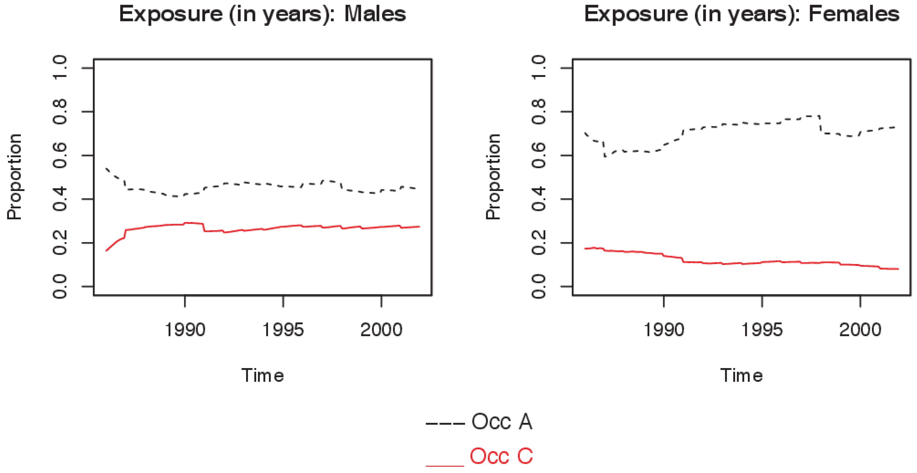
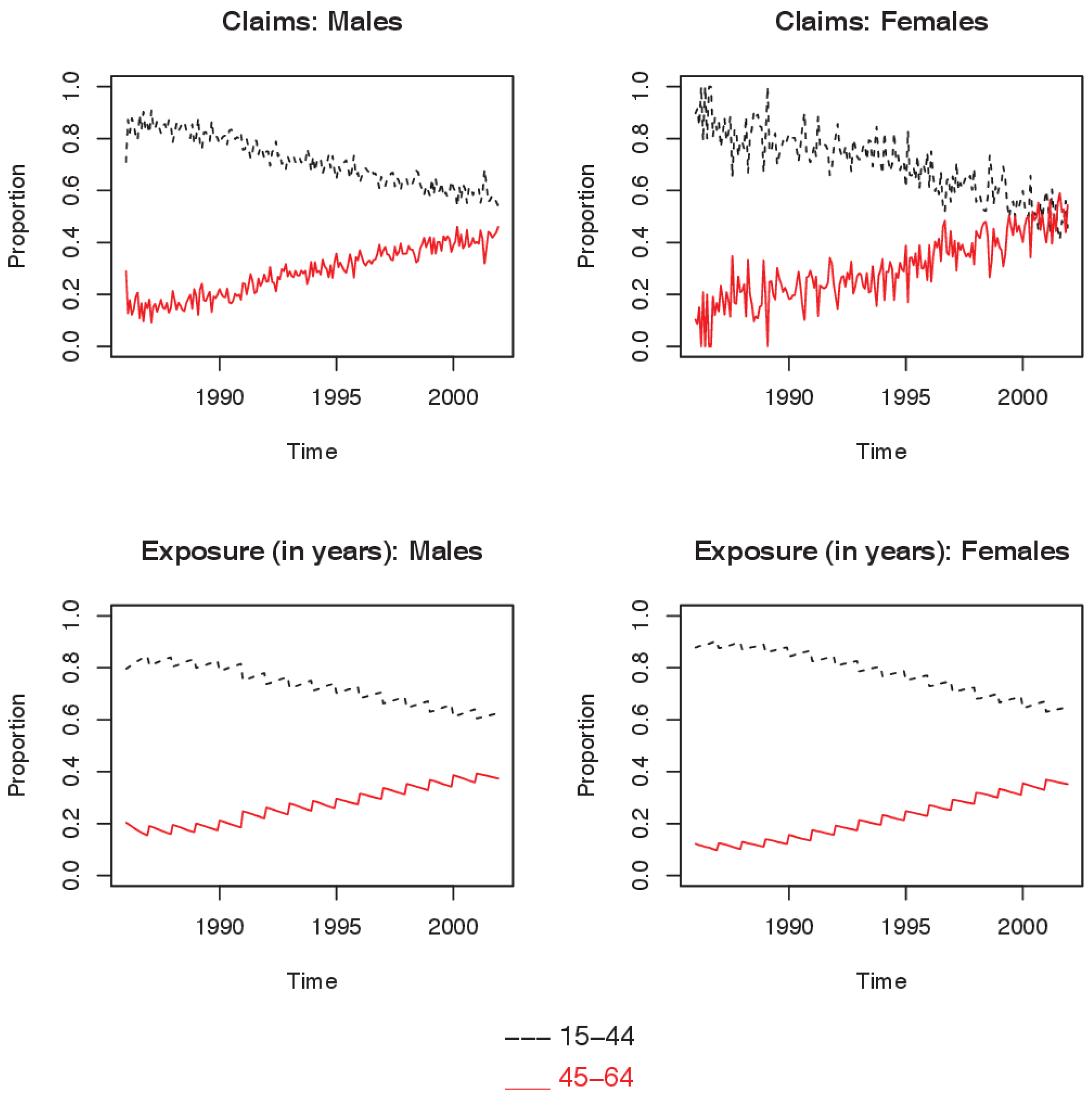
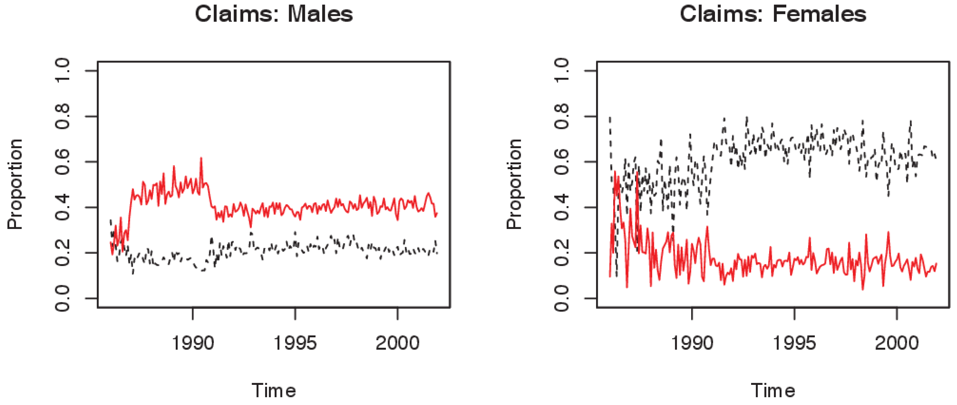
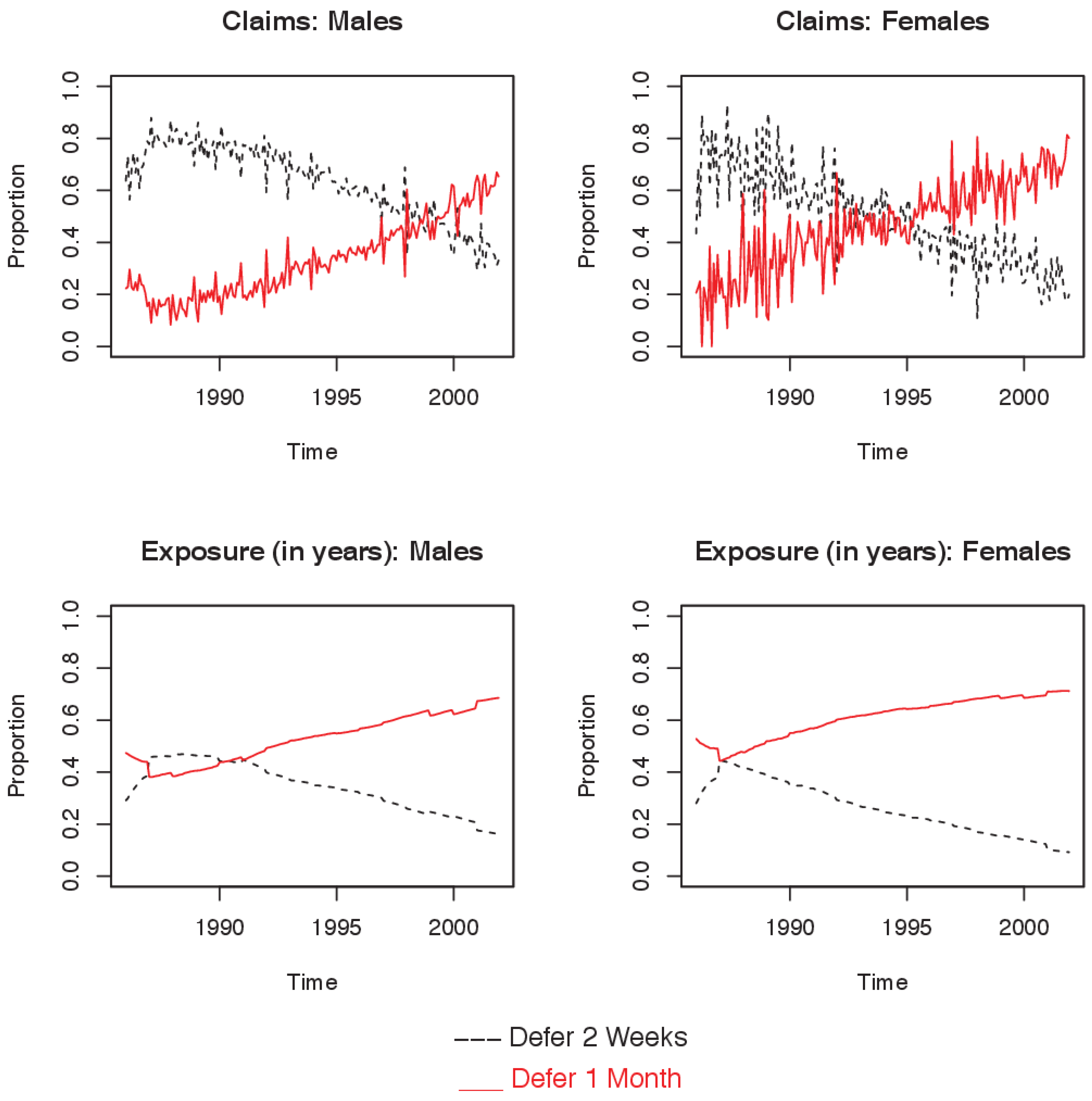
Notably, the proportions reported in Table 2 are based on exposure and claims data over the whole observation period (1986–2001) and do not provide an indication of change over time. Figure 1 shows how the proportion of the data in each of the age groups for both males and females has changed over the observation period. It is clear that the proportion of both claims and exposure for the 15–44 age group has been steadily decreasing while that of the 45–64 age group has been increasing over the period of observation, reflecting a more uniform population distribution exposed to DII. Plots of proportions for occupation class and deferment period are provided in the appendix.

In accordance with prior research [1,3,7,9], the economic indicator used in this study is the unemployment rate. While three other economic indicators were initially considered—namely, change in per capita gross domestic product, number of job vacancies, and number of job advertisements, the preliminary results from all four indicators were not dissimilar. For comparability with other studies, we chose unemployment rate as a proxy for economic conditions in Australia 9.

Table 3. Summary statistics of monthly unemployment rate over the period 1986–2001.

Age	15–44	45–64	All
Males
Minimum	5.32	3.87	4.92
Maximum	14.29	9.62	12.71
Median	9.06	5.84	8.04
Mean	9.25	6.2	8.27
Standard deviation	1.92	1.49	1.76
Females
Minimum	6.2	2.92	5.19
Maximum	12.82	7.02	11.4
Median	9.05	4.48	8.03
Mean	9.16	4.75	8.06
Standard deviation	1.48	0.91	1.36

All figures are percentages. The unemployment rate used in the analyses by occupation class and deferment period is the overall unemployment rate by sex.

provides summary statistics for the unemployment rate.

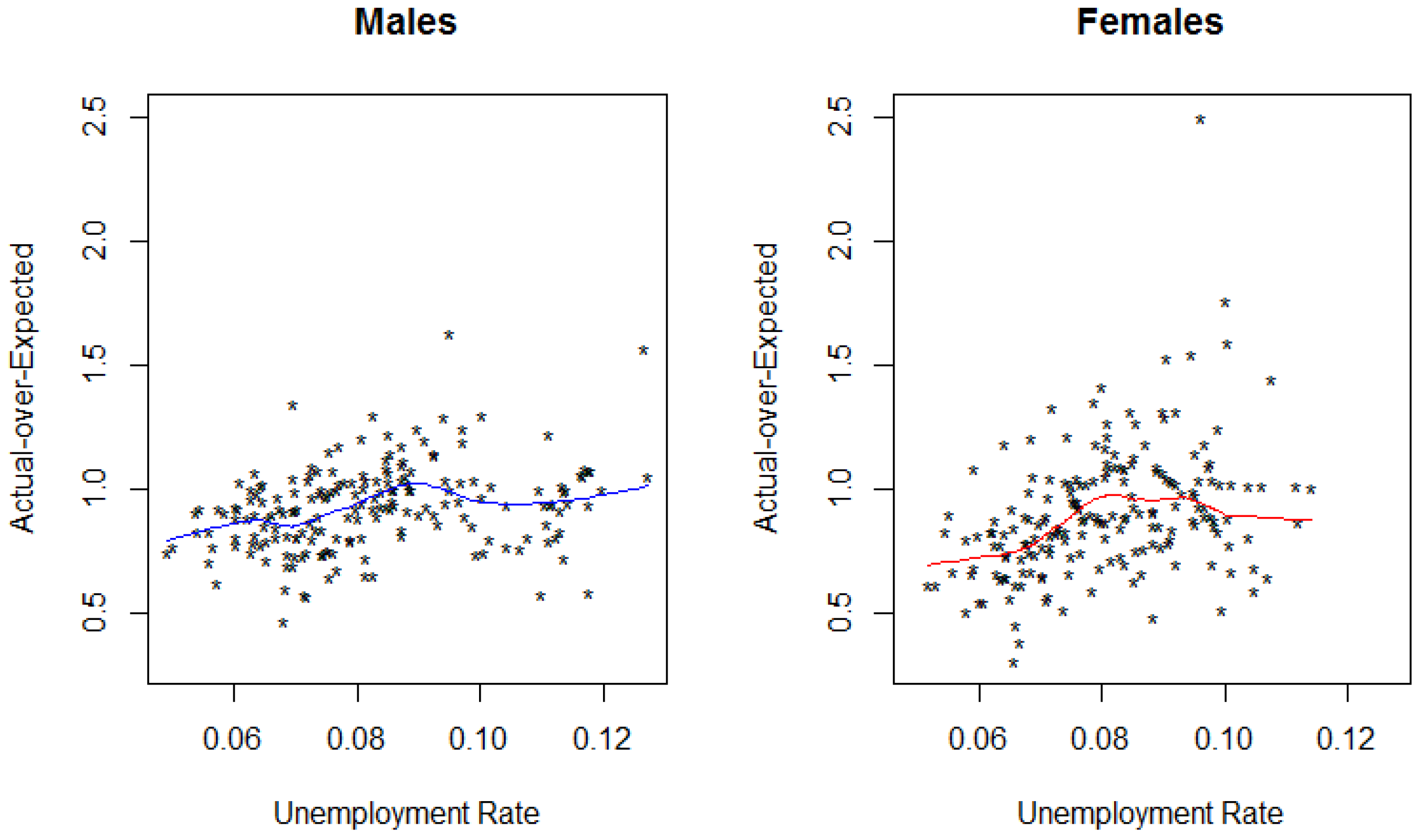
The relationship between the A/E ratio and unemployment rate is captured in Figure 2. The monthly data for A/E and unemployment rate indicate a weak positive relationship for both sexes, with a correlation coefficient of 0.28 and 0.37 for males and females respectively. The blue and red lines are the fitted lowess curves for males and females respectively 10.

3. Method

To analyse the effect of the economic changes on the DII business experience in Australia, a hurdle model with A/E as the response variable was employed. A description of and rationale for this model is given in Section 3.1. The expected number of claims by cause of claim was not available, so in order to analyse the relationship between economic changes and claim causes, we applied a multinomial logistic approach. Section 3.2 provides a rationale for selecting a multinomial logistic model and explains the modelling process. The results of the hurdle model and the multinomial model are combined to produce a picture of the impact of economic changes on claims arising out of four different claim causes.

3.1. Modelling A/E for All DII Claims

In an ideal world, the Expected used in the calculation of the A/E ratio would perfectly encapsulate the variation from all business characteristics. As described in Section 2, however, the Expected does not allow for all business characteristics, and so we must allow for characteristics omitted from the Expected in order to limit model bias. Moreover, Service [5] reports significant seasonality in the DII experience, thus any sensible model should also allow for this variation.

As stated in Section 2, after allowing for the underlying business characteristics and the structural effects on the A/E, any deviations from unity in the A/E should come from either exogenous influences (for example, changes in the economic conditions) or be due to unexplained variation.

In order to investigate the presence of a relationship between the economy and Australian DII experience, a hurdle model was fitted to the data. Hurdle models have been widely applied in actuarial claim count modelling, for example Boucher et al. [16] and Antonio et al. [17] as well as for alternative applications 11. The choice of the hurdle model was prompted by the composition of the data. Specifically, the A/E data is not available by individual claims or policies, but rather is aggregated by the various business characteristics. This monthly aggregated data is positively skewed and contains a substantial number of zeros. The zeros arise when, in a given group of policies with the same set of characteristics, no claims have been made for the month. A hurdle model allows us to deal with data of this type, and involves three steps. In the first step, and using the entire data set, we model the probability that in a given group at least one claim will arise. The following logistic model (Model A) was used to calculate the associated probabilities:

$$logit(Z_{mtk})=\alpha +{\beta }_i{U}_{mt}+{\delta }_m+{\gamma }_k+{ϵ}_{mtk}$$

(1)

where $Z_{mtk}$ is an indicator denoting whether there were any claims in the given group of policies (0 indicates no claims; 1 indicates at least one claim), for each month $(m)$, year $(t)$, and characteristics $(k)$ 12. α is an intercept. $U_{mt}$ represents the unemployment rate 13. ${\delta }_m$ captures the seasonality in A/E, ${\gamma }_k$ represents the factor of each business characteristic for which Expected is not available 14, and ${ϵ}_{mtk}$ is an error term. Model A is appropriately weighted by the exposure (in years) in each group 15.

The second step involves modelling the A/E. A subset of the original data, all groups where claims have occurred, is used for this step. Taking the natural logarithm of the A/E as the response, a linear model was fitted to the data. This log-linear model (Model B) takes the following form:

$$log(Y_{mtk})=\alpha +{\beta }_i{U}_{mt}+{\delta }_m+{\gamma }_k+{ϵ}_{mtk}$$

(2)

where $Y_{mtk}$ is the A/E in a given group of policies for each month $(m)$, year $(t)$ and characteristics $(k)$. The remaining terms have a similar interpretation as for Model A above. The linear model is also appropriately weighted by the exposure (in years) in each group.

The final step involved combining these two models. We label the combined model as the ‘hurdle’ model. The expected value of A/E is given by:

$$\begin{array}{cc}\hfill E(Y)& =Pr(Z=1)E(Y|Z=1)+Pr(Z=0)E(Y|Z=0)\hfill \\ & =Pr(Z=1)E(Y|Z=1)\hfill \\ & =\pi \mu \hfill \end{array}$$

(3)

where for ease of notation, and where no ambuiguity exists, Y and Z are used in place of $Y_{mtk}$ and $Z_{mtk}$ respectively; and π and μ are shorthand notations for $Pr(Z=1)$ and $E(Y|Z=1)$ respectively. The second step in the above formulation holds because the expected value of A/E is zero when there is no claim. An estimate of the expected value is therefore:

$$\widehat{E}(Y)=\widehat{\pi }\widehat{\mu }$$

(4)

where $\widehat{\pi }=\frac{exp(x^{\prime }\widehat{\theta })}{1+exp(x^{\prime }\widehat{\theta })}$ and $\widehat{\mu }=exp(w^{\prime }\widehat{\nu }+\frac{{\widehat{\sigma }}^2}{2})$ are estimates of π and μ and are obtained from the Models A and B. For ease of exposition, $\widehat{\theta }$ and $\widehat{\nu }$ are used to denote the vector of coefficient estimates from the logistic and log-linear model respectively, while x and w denote the corresponding vectors of explanatory variables. ${\widehat{\sigma }}^2$ is the residual mean square of the log-linear model.

In order to estimate confidence intervals for π, μ, and $E(Y)$, model-based bootstrap resampling was applied (e.g., see [20]) 16.

The model described above was fitted to fifteen policy sub-groups, specifically: males and females, and also males and females disaggregated by age group (two groups each: ages 15–44 and ages 45–64), occupation class (three for males: A, C and D; and two for females: A and C) and deferment period (two groups each: two weeks and one month).

3.2. Modelling A/E by Cause of Claim

Due to a lack of Expected data it is not possible to apply the model of Section 3.1 to cause of claim data, rather, a multinomial logistic model is adopted for the analysis by cause of claim. Claims experience data are grouped into four broad categories derived from the World Health Organisation’s coding system:

• Accidents;
• Mental Disorders;
• Musculoskeletal Diseases; and
• All Other.

The multinomial logistic model (Model C) takes the following form:

$${\eta }_{mtkp}=\log \left(\frac{{\pi }_{mtkp}}{{\pi }_{mtk1}}\right)=\alpha +{\beta }_p{U}_{mt}+{\delta }_m+{\gamma }_m+{ϵ}_{mtkp}$$

(5)

where ${\beta }_p$ is a vector of regression coefficients for $p=2,3,4,$ being the three categories of claim cause excluding the baseline category. ${\eta }_{mtk1}$ is the log odds corresponding with the baseline (category 1, which corresponds with claims arising from accidents). The remaining terms have a similar interpretation to Model A 17. The estimated probabilities of a claim arising from each of the four causes, given that a claim has occurred, were output from the fitted model 18. As for the hurdle model, a model-based bootstrap was employed to obtain the 95% confidence intervals of the relative probabilities of each claim cause.

To ascertain the extent of the relationship between unemployment rate and the number of claims by cause, we combine the results of the hurdle model of Section 3.1 with the multinomial logistic model. This is achieved as follows: first, we set an arbitrary base of 1000 claims for all causes at a 3% unemployment rate, which corresponds with the lowest observed unemployment rate during the period 1986–2001; second, we estimate the expected total claims at each rate of unemployment relative to the base at 3% unemployment, through application of the hurdle model of Section 3.1 19; third, the fitted probabilities from Model C are applied to the total expected claims to produce estimates of the claim numbers in each of the four categories at each rate of unemployment.

For example, consider the relationship between unemployment rates and DII claims for males. We assume that there were 1000 claims at 3% unemployment rate. Using the results of the hurdle model, at 15% unemployment there would be approximately 1400 claims. Then using the estimated probabilities from Model C, these claims would be divided between the four claim causes (at each level of unemployment). For example, at 15% unemployment, of the 1200 claims arising from males, (approximately) 725 would be accident-related, 140 would be from mental illness, 360 from musculo-skeletal causes and 180 from all other causes.

As before, 95% confidence intervals for the number of claims are obtained by multiplying the bootstrapped results (from the hurdle and the multinomial logistic model) in the same manner.

4. Results

4.1. A/E for All DII Claims

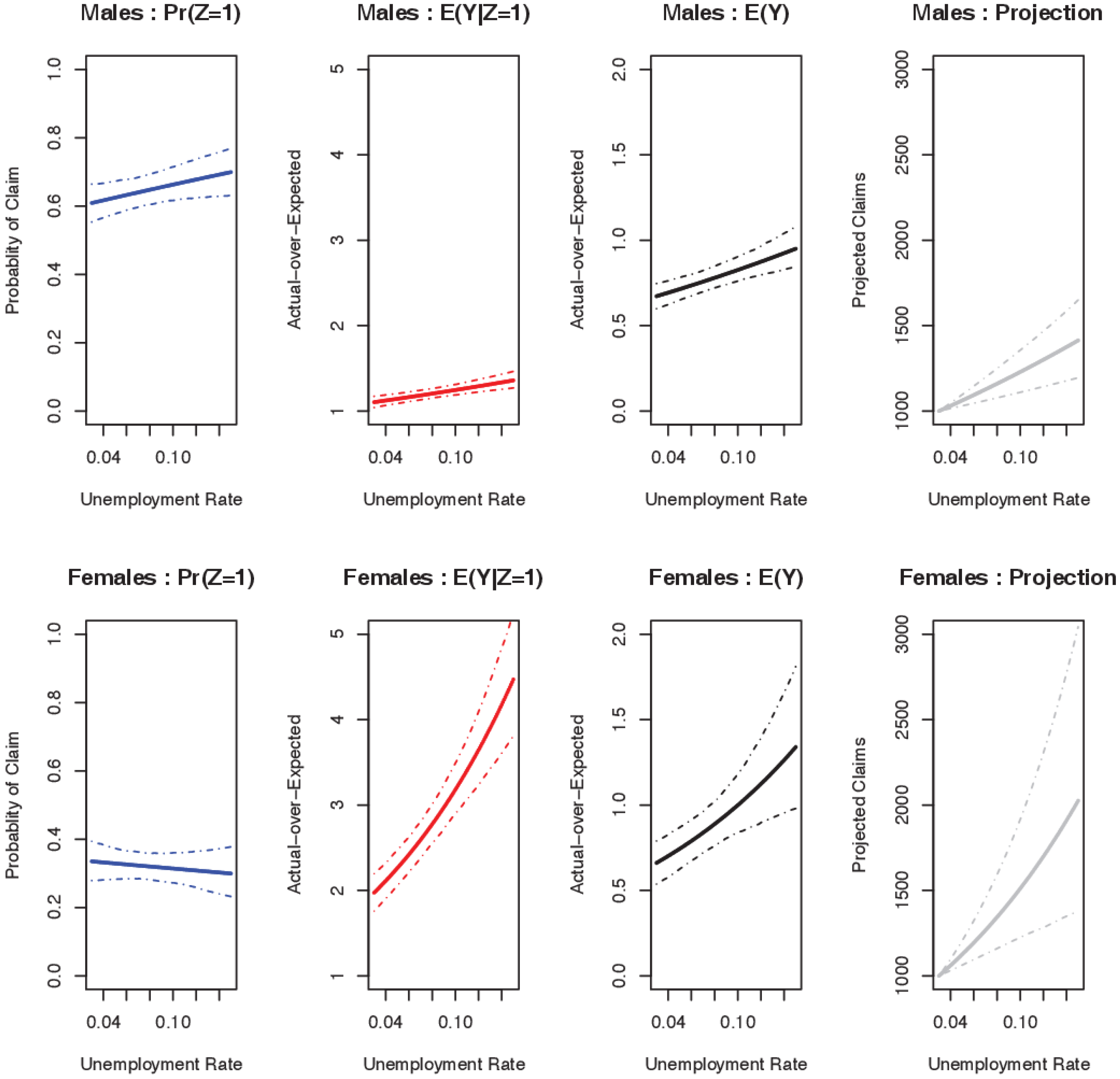
Figure 3 provides an illustration of the results of the steps of the hurdle model 20. From left to right, the figure presents the results for the logistic model (Model A), fitted results of the log-linear model (Model B), the expected A/E for the combined hurdle model, and finally the projected claim numbers relative to a base of 1000 at 3% unemployment. The unemployment rate is selected to vary from 3% to 15% in the figures.

The far left panel in Figure 3 shows the probability that at least one claim occurs, which increases with increasing unemployment for males, and decreases marginally for females. However, the effects are not statistically significant in either of the cases. The next panel illustrates that given at least one claim, A/E rises with increasing unemployment, and substantially more so for females. As the Expected is estimated independently of the unemployment rate, a change in A/E corresponds with a change in the number of actual claims. As shown in

Table 4. Coefficient estimates for unemployment rate in the hurdle model.

	Males		Females
	Log-Linear	Logistic	Log-Linear	Logistic
Entire Population	5.894 *	1.731 **	−2.309	6.815 **
	(2.373)	(0.356)	(1.881)	(0.801)
Age Groups
15–44	2.314	1.388 **	4.531 **	5.465 **
	(1.827)	(0.366)	(1.645)	(0.891)
45–64	−0.472	3.108 **	−23.800 **	14.138 **
	(1.728)	(0.580)	(2.343)	(1.739)
Occupation Classes
A	6.093 **	1.397 *	2.807	7.307 **
	(1.503)	(0.545)	(1.811)	(0.954)
C	−8.805 **	3.653 **	−6.734 **	12.995 **
	(2.175)	(0.492)	(1.796)	(1.647)
D	11.160 **	6.140 **	NA
	(2.107)	(0.607)
Deferment Periods
Two Weeks	10.250 **	2.702 **	12.802 **	3.997 **
	(2.066)	(0.405)	(1.597)	(1.101)
One Month	−4.119 *	0.64	−14.181 **	8.020 **
	(1.643)	(0.496)	(1.717)	(1.061)

Statistical significance is marked with stars. * at 5% and ** at 1% level of significance.

, the effect appears to be statistically significant for both sexes.

The next panel shows the fitted A/E for the combined hurdle model. The effect of an increasing unemployment rate leads to an increase in the expected A/E for both males and females (and therefore, an increase in expected claims), with the impact in the case of females (0.66 to 1.35) being greater than in the case of males (0.67 to 0.95). The final panel (far right) presents the same results as those in the third panel, this time relative to a base number of claims of 1000 at 3% unemployment rate. The panel presents the evolution in the number of claims as unemployment increases, along with a 95% prediction interval to illustrate the associated prediction uncertainty. In aggregate, the results indicate that DII experience in Australia behaves in a counter-cyclical manner for both males and females, with the effect being more pronounced for females (that is, claims increase with increasing unemployment) 21.

The coefficients of the unemployment rate from the log-linear and logistic models are given in Table 4 22.

The importance of the model results can be best conveyed through examination of the impact of each factor on the predicted claim numbers as the rate of unemployment changes.

Table 5. Average change in number of claims for 1% increase in unemployment rate.

		All Claims	Accident	Mental Illness	Muscolo-Skeletal	All Other
Entire Population	Males	34.5 *	34.1 *	3.3	2.1	−5
	Females	85.5 *	45.5 *	19.2 *	22.2	−1.5
Age Groups
15–44	Males	21.8 *	25.7 *	1.8	0.2	−5.8 *
	Females	120.7 *	36.8 *	21.3 *	65.4 *	−2.8
45–64	Males	35.6 *	30.0 *	5	4.3	−3.8
	Females	−14.3	31.4 *	3.3	−44.7 *	−4.3
Occupation Classes
A	Males	41.8 *	46.7 *	10.8 *	−17.6 *	1.9
	Females	150.7 *	50.4 *	32.4 *	60.6 *	7.3
C	Males	13.7	35.2 *	1.8	−18.6 *	−4.7
	Females	146.4 *	45.9 *	16.6	77.8	6.3
D	Males	175.3 *	160.1 *	1.4	9	4.9
Deferment Periods
Two Weeks	Males	71.4 *	72.4 *	2	−1.8	−1.2
	Females	207.0 *	74.6 *	27.6 *	96.7 *	8.1
One Month	Males	−5.2	30.6 *	0.2	−30.1 *	−5.9 *
	Females	9.4	14	6.5	−8.3	−2.9

Statistical significance at the 5% level is marked with a star-*. For the purpose of this table we report that a factor is statistically significant if the 95% bands corresponding with the claim estimate at 3% unemployment do not overlap with the bands corresponding with the claim estimates at 15% unemployment. That is, statistical significance as reported here does necessarily imply that a 1% change in unemployment rate corresponds with a statistically significant change in claims, but rather that there is a significant change in claims over the range of unemployment rates considered. Separate models were fit for different characteristics, and as a consequence the estimates for the average change in claim numbers for the entire population may fall outside the estimates corresponding with individual characteristics.

presents these results, along with a decomposition by cause of claim.

4.2. A/E by Cause of Claim

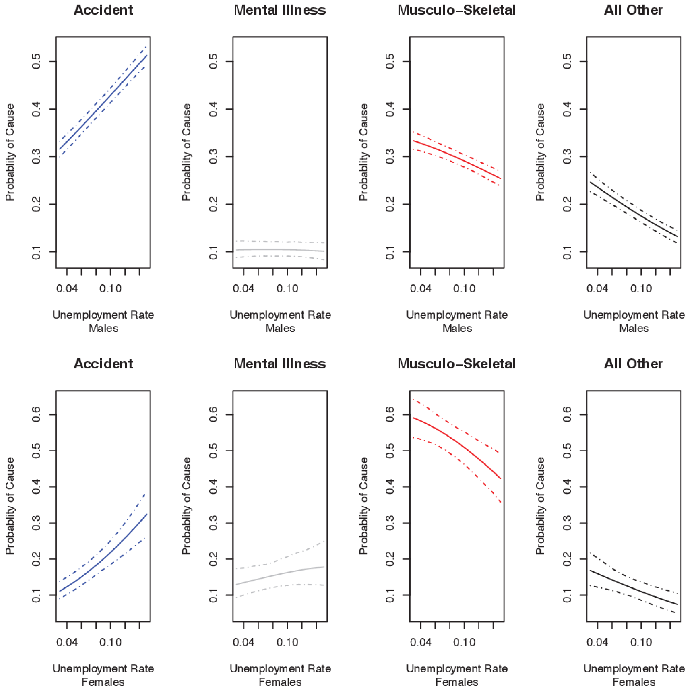
The results of the multinomial logistic model by sex are displayed in Figure 4. The top and bottom panels give the result for males and females respectively. The figures present the probabilities of a claim arising from one of the four causes at a given rate of unemployment, conditional on a claim having occurred. The results indicate that for both sexes, an increase in the unemployment rate leads to: an increase in the relative probability of a claim arising from accidents; a negligible change in the relative proportion of claims from mental disorders; and a relative decrease in the probability of that claims will arise from musculo-skeletal and all other causes 23.

In Section 4.1 it was shown that increases in the unemployment rate were accompanied by statistically significant increases in A/E for both males and females. In order to illustrate the effect of increasing unemployment on the number of claims arising from each cause, as for Section 4.1, we start with a base assumption of 1000 claims at an unemployment rate of 3%. First, using the hurdle model results, we predict the total number of claims for each unemployment rate. 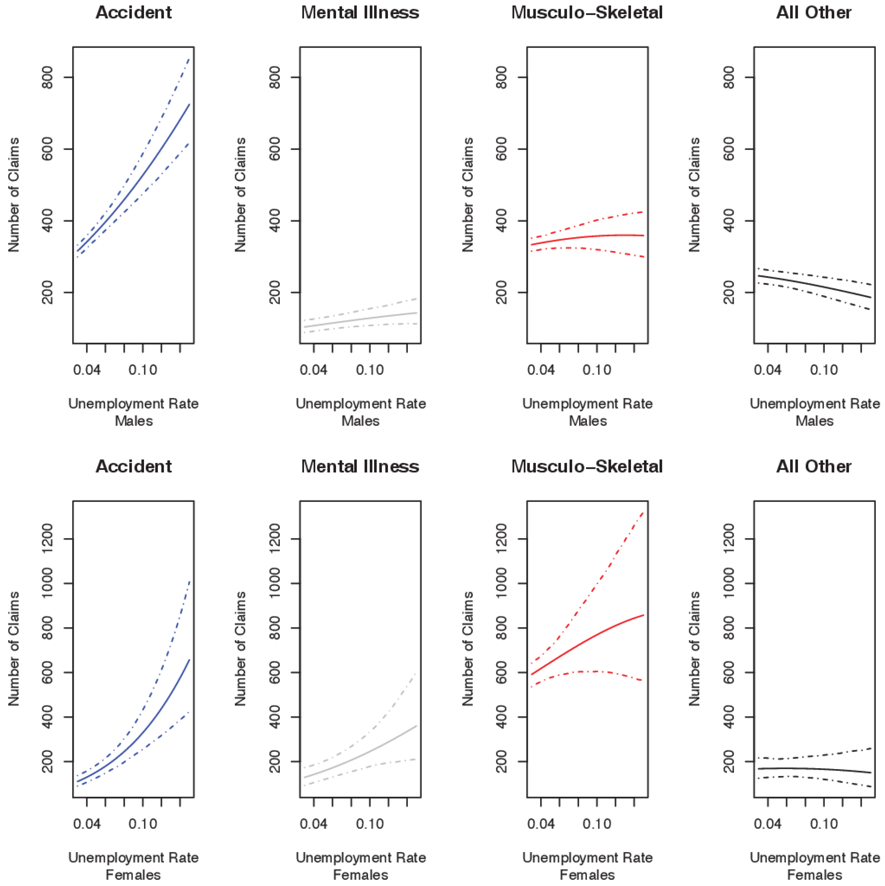Next, we use the conditional probability by cause results represented in Figure 4, to apportion the total number of claims amongst the four claim causes. The resulting claims arising from each cause are shown in Figure 5. Note that the counter-cyclical behaviour of claims dictate that the absolute number of claims incurred increases as the unemployment rate rises.

In Figure 5 the number of claims arising due to accident increases markedly with rising unemployment, and dominates the results. There is a negligible increase in the number of mental illness claims for males, but a significant increase for females. Musculo-skeletal claims for males are flat, while all other claims decline slightly. Although musculo-skeletal claims for females appear to rise with increasing unemployment, wide prediction intervals indicate marginal significance at best. The results of the modelling undertaken and described throughout this paper are summarised in Table 5, which presents the expected change in the number of claims in the event of a 1% increase in the unemployment rate 24.

The results are presented in this way for two reasons. First, it provides a clear indication of the magnitude of the impact of changes in unemployment on claim numbers, thereby providing a gauge of the level of economic significance. Second, it shows how aggregate claim numbers can be decomposed into claim causes, thereby providing insight into the possible determinants of the observed counter-cyclical claim pattern.

In the remainder of this section we provide some observations on the key findings presented in Table 5. As shown in Figure 3, it is clear that an increase in unemployment rates leads to a much greater rise in female claims than male claims. For both sexes the majority of the increase is due to claims associated with accidents. Mental illness and musculo-skeletal claims also increase for females, though the significance of the rise in musculo-skeletal changes is marginal at best, and in both cases the magnitude of the increases are small relative to accident claims. Decomposition of the female results by age, however, tells a different story.

In contrast to the female results by age, which are discussed below, results by age group for males show little difference between 15–44 and 45–64 years old. For both groups claim growth is almost exclusively associated with accidents. While there is some evidence of a statistically significant decrease for ‘all other’ claims for 15–44 males, the magnitude of the decrease is not material relative to the rise in claims associated with accidents. For females there is a dramatic difference between age groups, most notably for musculo-skeletal claims, which rise markedly for 15–44 years old while the claims for the 45–64 years old show a significant drop as the unemployment rate rises. This large difference raises questions as to plausible reasons. Parental responsibilities and corresponding financial pressures are higher in the younger age group, which could plausibly impact on the incentives to claim as the economy slows. Higher unemployment discourages workforce participation, and for older women who have lower rates of workforce retention than men, this may result in lower DII exposure and consequently lower claims.

For males there is a clearly large increase in claims from accidents for all occupation classes when unemployment rises. Medium and heavy manual workers (occupation class D), in particular, experience a particularly large increase in claims. While we cannot be certain of the reasons for this pattern, it is plausible that a decline in employment rates and economic conditions leads to poorer risk management, and therefore a greater rate of accidents. On the other hand, perhaps not all of these claims are legitimate; as DII is relied on for work-related cover by blue-collar self-employed, there may be increased moral hazard when the economy is slowing. The ‘hidden’ disabled, as described early in this paper, may also be partly responsible for the observed results. As for males, females in white-collar and light manual professions have higher accident claims as unemployment rises. In contrast to male white-collar workers, white-collar women experience a large rise in musculo-skeletal claims with increasing unemployment.

A one-month deferment period requires that the disability persists for a longer period prior to benefits commencing when compared to a two-week deferment. It is possible that these results are suggestive, in part, of moral hazard. For example, it is not unreasonable that fraudulent claims may be associated with minor causes that are more likely to be sustained for shorter rather than longer periods.

5. Discussion

The results of the analysis of Australian DII claim experience and economic conditions over the period 1986–2001 reveal that claim incidence increases with increasing unemployment rates. On average, a 1% increase in the unemployment rate is associated with a 2.3% increase in claims for males and a 5.7% increase in claims for females, though the increase among females appears concentrated in the 15–44 years old age group. This observed counter-cyclical pattern of claim incidence is consistent with findings reported for the United States [7,8,9] and for South Africa [3].

Analysis by cause reveals that the composition of claims changes as unemployment rates rise. An increase in unemployment corresponds with an increase in the relative probability of claim from accident, and a fall in the relative probability musculo-skeletal claims and all other claim causes. A 1% increase in unemployment is associated with a 1.6% and 1.8% increase in the probability of claim from accidents, a 0.7% and 1.4% decrease in the relative probability for musculo-skeletal claims, and a 1% and 0.4% decrease in the relative probability for the ‘all other’ claims , for males and females, respectively. The relative proportion of claims arising from mental illness does not appear to be affected by changes in unemployment. When the results of the hurdle model and multinomial logistic model are combined, it is apparent that the unemployment rate is associated with a marked increase in the absolute claim numbers from accident, with more modest increases in mental illness and musculo-skeletal claims, and declines in claims arising from all other causes.

The results presented here are in contrast to prior research which indicates that accident claims tend to be pro-cyclical in nature [4,12]. A plausible argument is that in uncertain or difficult economic times, policyholders may lodge accident claims for minor causes that they would not otherwise report during economic upturns, in accordance with the theory put forward by Schriek and Lewis [3]. Moreover, in accordance with prior research [2], claim numbers from sickness (mental illness and musculo-skeletal taken together) tend to increase with increasing unemployment.

The decomposition by claim type and policy characteristics raises some interesting findings. The most notable include the following claim patterns as unemployment rates rise: an increase the musculo-skeletal claims for younger women but a commensurate decrease for older women, a dramatic rise in accident claims for medium and heavy manual male workers, and a rise in accident claims offset by a fall in musculo-skeletal claims for males with one-month deferment periods. Although the analysis by policy characteristic does not offer reasons for the observed relationships, in the previous section we provide some limited speculation on these findings.

Regardless of the reasons behind the observed patterns, analysis indicates that during periods of increasing unemployment, DII claims tend to rise, particularly claims associated with accidents, claims from policy holders with shorter deferment periods, and claims from medium and heavy manual male workers. Although predicting economic downturns can be fraught with challenges, closely monitoring and anticipating changes to unemployment rates could potentially improve life insurer DII claim predictions, pricing and reserving.

The magnitude of the results in terms of increased claim rates, and the consequent implications to insurance operations and labour productivity, suggest the need for more research in this area to attempt to isolate the reasons for these findings. In particular, there is a need for additional analysis and modelling with more contemporary data that reflects the current distribution of cause of claims 25.

One of the major limitations of this study is the data period of the Australian DII business, namely 1986–2001 26. While the data is indeed dated, and the corresponding conclusions of the study may have changed in recent years (for example there is anecdotal evidence of an increasing trend of claims arising from mental illness), this study does provide a useful methodology of analysing the DII business, which can be extended to other insurance areas.

In conclusion, DII claims in Australia exhibit a counter-cyclical pattern. While the data could be interrogated further to explore DII business, the analysis presented here lends credence to the argument that DII claims may sometimes be used as a substitute for participation in the workforce [6]. Our findings give support to the hypothesis that there is a behavioural component behind DII claim incidence, and our results show that the magnitude of the change in claims incidence in periods of declining economic conditions could have a material impact on insurer business.