
Immunization and Hedging of Post Retirement Income Annuity Products

CEPAR and School of Risk and Actuarial Studies, UNSW Business School, University of New South Wales, 2052 Sydney, Australia
*
Author to whom correspondence should be addressed.
Risks 2017, 5(1), 19; https://doi.org/10.3390/risks5010019
Submission received: 17 January 2017
/
Revised: 5 March 2017
/
Accepted: 13 March 2017
/
Published: 16 March 2017
(This article belongs to the Special Issue Designing Post-Retirement Benefits in a Demanding Scenario)
Abstract
:Designing post retirement benefits requires access to appropriate investment instruments to manage the interest rate and longevity risks. Post retirement benefits are increasingly taken as a form of income benefit, either as a pension or an annuity. Pension funds and life insurers offer annuities generating long term liabilities linked to longevity. Risk management of life annuity portfolios for interest rate risks is well developed but the incorporation of longevity risk has received limited attention. We develop an immunization approach and a delta-gamma based hedging approach to manage the risks of adverse portfolio surplus using stochastic models for mortality and interest rates. We compare and assess the immunization and hedge effectiveness of fixed-income coupon bonds, annuity bonds, as well as longevity bonds, using simulations of the portfolio surplus for an annuity portfolio and a range of risk measures including value-at-risk. We show how fixed-income annuity bonds can more effectively match cash flows and provide additional hedge effectiveness over coupon bonds. Longevity bonds, including deferred longevity bonds, reduce risk significantly compared to coupon and annuity bonds, reflecting the long duration of the typical life annuity and the exposure to longevity risk. Longevity bonds are shown to be effective in immunizing surplus over short and long horizons. Delta gamma hedging is generally only effective over short horizons. The results of the paper have implications for how providers of post retirement income benefit streams can manage risks in demanding conditions where innovation in investment markets can support new products and increase the product range.
1. Introduction
Post retirement benefits in the form of an income benefit, either as a pension or an annuity, provide a hedge against both investment risks and mortality risk for an individual. Pension funds and life insurers offer these pensions and annuities generating long term liabilities linked to both interest rates and aggregate improvements in longevity of its pensioners and annuitants. Risk management of these pensions and life annuity portfolios needs to take into account interest rate risks as well as longevity risk. The risk arises from a mismatch in changes in the value of assets and liabilities as interest rates and future mortality expectations change, resulting in a potentially adverse change in portfolio surplus.
Interest rate risk immunization has a long tradition in the optimal selection of portfolios of bonds to match insurance liabilities in both the actuarial and the financial literature. The classical approach to interest rate immunization of an insurer’s liabilities is Redington’s theory of immunization which is based on a deterministic shock to a flat yield curve [1]. Fisher and Weil [2] extended the analysis to a non-flat yield curve. Extensions of interest rate immunization to multiple liabilities and non-constant shocks as well as the application of linear programming techniques to select immunized bond portfolios are presented in Shiu [3,4,5].
Immunization has been applied to mortality risk. Tsai and Chung [6] and Lin and Tsai [7] derive duration and convexities for a range of life annuity and life insurance product portfolios. They then construct portfolios of life annuity and life insurance products that immunize mortality risk, a form of natural hedging. They consider alternative duration and convexity matching strategies with differing assumptions for mortality shocks. Lin and Tsai [7] use Value-at-Risk measures for the time zero surplus and the Lee-Carter model to assess the effectiveness of the immunization strategies. They consider instantaneous proportional and parallel shifts in the one-year survival probability and the one-year death probability . Tsai and Chung [6] apply a linear hazard transformation to mortality immunization allowing a proportional and parallel shift in mortality rates. Only mortality shocks and portfolios of life annuity and life insurance products are considered.
Luciano et al. [8] develop delta-gamma hedging for annuity providers allowing for both stochastic interest rates and stochastic mortality rates. They use zero coupon bonds and zero coupon survival bonds as the assets in the hedging strategies and pure endowment contracts as the liability. Using delta and gamma risk measures based on their stochastic interest rate and mortality models, they select portfolios that have zero delta and zero gamma for both mortality and financial risk.
We consider the immunization of a life annuity portfolio and the extension of linear programming approaches to the selection of fixed-income and longevity bonds. We consider only static hedging since this provides a consistent approach for comparison. We use simulation and a range of risk measures including volatility, value-at-risk and expected shortfall for the portfolio surplus and comparisons of these risk measures to assess the effectiveness of the immunization and hedging strategies. Both duration and convexity matching approaches, commonly used in fixed interest portfolio selection, as well as delta-gamma hedging, commonly used to hedge derivatives, with stochastic interest rate and mortality models are considered and compared. We implement immunization and delta-gamma hedging for an asset portfolio consisting of fixed-income coupon and annuity bonds as well as longevity linked bonds. Annuity bonds pay a level stream of principal and interest and have the potential to better match life annuity cash flows. Longevity bonds link payments to mortality.
We consider traditional immunization approaches using duration and convexity since this is standard in measuring risk for fixed income portfolios and has direct relevance for bond portfolios to match life annuity cash flows. Delta-gamma hedging, that is usually most relevant for derivative cash flows, have the potential to select bond portfolios when both interest rate and longevity risk are to be hedged. Bonds are derivatives of the underlying interest rates, or in the case of the longevity bonds, both the underlying interest rates and mortality rates.
The main results are that longevity bonds are very effective in immunizing longevity risk. Only a small number of both short and long maturity longevity bonds are required to immunize life annuity liabilities. Annuity bonds better match the expected cash flows of life annuity liabilities over coupon bonds, but longevity bonds better manage the risk. Over short horizons both immunization and delta-gamma hedging are effective in selecting bond portfolios for life annuities. Over longer horizons, immunization is more effective. Delta-gamma hedging is based on stochastic models for both interest rate and mortality risk and is less robust to these underlying risks over longer horizons as compared to immunization.
This paper is structured as follows: Section 2 describes the modelling framework for the underlying mortality model and interest rate model respectively. Section 3 outlines the construction of portfolios including derivation of pricing, delta, gamma, duration and convexity results. Section 4 provides details of the bond portfolios used in the immunization and hedging based on both available and hypothetical bonds. Section 5 presents the linear program used for selecting the immunization bond portfolios and compares the cash flows of the annuity liability with the bond portfolios. Section 6 presents the linear program used for the delta-gamma hedging strategies and compares the cash flows for the bond portfolios with the annuity liability. Section 7 uses the stochastic models to compare the hedge performance of the immunization and hedging bond portfolios. Section 8 concludes the paper.
2. Stochastic Models and Calibration
The risk of adverse portfolio surplus for a life insurer with a life annuity portfolio arises from adverse changes in the value of the assets relative to the value of the liabilities. Traditional immunization approaches aim to minimize this risk using deterministic shocks to yield curves and revaluing the assets and the liabilities. Asset portfolios of bonds are selected to minimize the changes in surplus. Delta-gamma hedging selects assets by matching the sensitivity of asset and liability values to changes in the underlying financial and demographic variables that determine these values. This hedging uses stochastic models of the underlying risks.
In order to compare these different approaches, we develop stochastic mortality and interest rate models. The models are used to derive pricing formulas to value the assets and liabilities as well as to quantify mortality and interest rate risk for a life annuity portfolio. By using simulation of the portfolio surplus of an annuity portfolio we are able to compare delta-gamma hedging strategies with immunization strategies. To do this we compare the hedge effectiveness of these approaches by simulating the surplus of a life annuity fund with asset portfolios selected using both immunization and delta-gamma hedging. We then compute risk statistics for the surplus using standard risk measures of volatility, value-at-risk and expected shortfall. The effectiveness of these approaches are then compared based on the reduction in these different risk measures for the different portfolios.
The risk factors in the interest rate model are assumed to be independent of those in the mortality model. We use Australian mortality and interest rate data to calibrate the models. Australian mortality and interest rate experience is representative of many developed economics. Australia has a well developed bond market including coupon bonds and annuity bonds.
2.1. Mortality Model
The mortality model is a two-factor Gaussian stochastic Makeham model based on Schrager [9]. This has been used in a number of studies of longevity risk. The model is affine and gives closed form solutions for survival probabilities. The mortality intensity for an individual aged x at time t is given by:
where and are the base and age-dependent mortality risk factors respectively. As time passes an individual ages so that the age x is increasing as time increases.
The stochastic differential equations for the mortality risk factors are:
where for ; and ; and we assume the two mortality factors are independent, consistent with the assumption made in Biffis [10], Blackburn and Sherris [11] and Wong et al. [12].
Pricing longevity bonds and life annuities requires the mortality dynamics under a risk-neutral measure . The longevity risk market is not liquid enough to calibrate risk premiums and there is no agreed basis for the size of these risk premiums. Since the risk premium will impact both assets and liabilities and will offset to a significant extent, and it will not explicitly impact the risk measures used, it is assumed zero, and we use the real world measure for pricing and risk measures. This is the assumption made by Luciano et al. [8].
Based on the affine framework, the forward survival probability is
where , and are of the forms:
with boundary conditions , and .
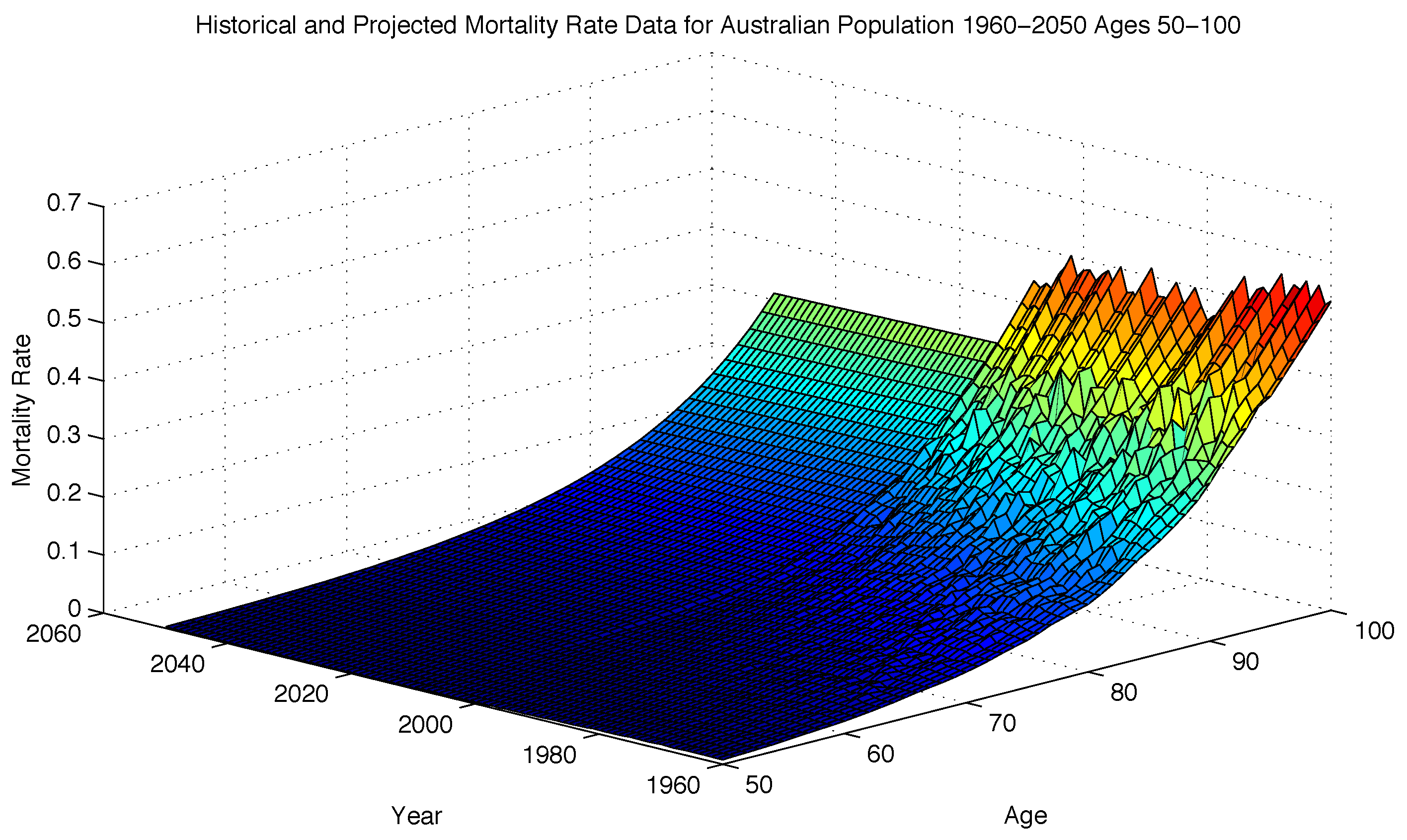
The mortality model is calibrated to Australian Mortality Data for males aged 50–100 and years 1960–2009 obtained from the Human Mortality Database [13]. We used the estimation methods in Koopman and Durbin [14] and Wong et al. [12] based on the Kalman filter. The calibrated parameters for the mortality model are shown in Table 1.
Figure 1 shows the historical mortality rate with the projected mortality rates from the calibrated model. Mean absolute relative error (MARE) range between and for the fitted ages from 50 to 100, similar to Schrager’s results when calibrated to Dutch mortality data.
2.2. Interest Rate Model
The instantaneous interest rate is modelled as a single-factor Cox-Ingersoll-Ross (CIR) process with its dynamics under the risk neutral measure given by:
where is the speed of mean reversion of , is the long-run mean of , is the volatility of the short rate process, and needs to be satisfied to ensure the process is positive [15].
The dynamics of the interest rate under the measure, where the over-bar is used for the real world parameters, is given by:
where
is the market premium of interest rate risk and we assume to be a function of so that is a constant.
The forward zero coupon bond price is given by:
where and are given by:
with
with boundary conditions and .
The CIR interest model parameters are estimated from zero-coupon bond yield data for 40 different maturities (3, 6, 9, ..., 117, 120 months) using daily data from 4 January 1993 to 31 July 2014 along with daily short rate data. The zero-coupon bond yield and short rate data were obtained from the Reserve Bank of Australia.
The estimation technique is adopted from Rogers and Stummer [16] and Kladıvko [17]. It uses the General Method of Moments (GMM) approach with moment conditions. M is the number of different maturities for the zero coupon bond data, in our case . The first M moments fit the yield curve allowing estimation of the implied market interest rate risk premium. The last 2 moments fit the time series data of short rates and match the mean and variance of the real world CIR interest rate process. This calibration method estimates the model parameters as well as the market risk premium using both yield curve and short rate data. The parameter estimates were found to be consistent across time when we fit the model to data for different time periods using the GMM. Fitting the model only to the yield curve data results in unreasonable estimates for the parameters.
The calibrated parameters of the interest model are shown in Table 2.
The model parameters imply an Australian long-term interest rate of approximately . The parameters under the measure are and . The standard errors for the parameter estimates are derived using numerical approximation of the asymptotic variance matrix as in Mátyás [18].
Figure 2 shows the 50-year yield curve used for product pricing.
3. Life Annuity Immunization
Our approach is to consider the immunization and hedging strategy from the perspective of an annuity provider issuing whole-life annuities with level monthly payments to males aged 65 at 30 June 2014. All life annuities are single premium and the insurer invests these premiums into fixed-income securities and longevity-linked securities. Our focus is on interest rate and longevity risk and we do not include idiosyncratic mortality risk or basis risk. Risk is measured by considering the surplus distribution on the portfolio taking into account the assets and liabilities. Risk measures used are volatility of the surplus as well as value-at-risk and expected shortfall. The effectiveness of the different asset portfolios is assessed by comparing these differing risk measures. A portfolio that produces a lower value for these risk measures is considered as more effective in managing the risk.
The initial number of policyholders is 100, the coupon bonds have a face value of 100 and the payment amount for the annuity bonds and the longevity bonds is $1. These values are used for convenience and are in effect arbitrary. The important determinant of the bond portfolios selected is the weights in each of the assets.
We use linear programming to solve for the optimal bond portfolio allocation. The methods used are standard in the literature for selection of asset portfolios to match liability cash flows.The linear programming approach of Shiu [4] and Panjer et al. [19] is extended to include both interest rate and mortality risk. To reflect the situation in practice, we take into consideration a wide range of different fixed-income securities and select the optimal portfolios from these. We select portfolios from more than 60 coupon bonds and annuity bonds, including maturities and securities available in the market, along with hypothetical longevity bonds. The details of the bonds are covered in Section 4. We assume all securities are non-callable, and default free. Credit risk is assumed fully hedged and does not impact the interest rate or longevity risk analysis.
The immunization approach aims to match time weighted values or the duration of the assets and liabilities where values are determined using the current interest rates and mortality rates. In our implementation we follow the approach in Panjer et al. [19] which aims to minimize surplus risk of the portfolio based on the convexity of the cash flows, while matching duration. This is used for bond portfolio selection and this approach is consistent with fixed income approaches. For derivatives, risk is usually measured with sensitivities based on the delta and gamma of the underlying securities, which in fixed interest portfolio selection are equivalent to modified duration and convexity.
3.1. Duration, Convexity, Delta and Gamma
For the immunization we adapt the Fisher-Weil cash flow duration and Fisher-Weil convexity measures to longevity linked cash flows. We also use delta and gamma. These are defined in Table 3, Table 4 and Table 5 for the asset and liability cash flows. Table 3 gives the Fisher-Weil duration and convexity measures along with the delta and gamma definitions used for the assets.
Table 4 gives the formulae used for cash flow prices, dollar duration and dollar convexity of assets and liabilities used in Table 3. To indicate whether we use interest only bond cash flows or mortality dependent cash flows we use the index k for fixed-income securities and j for longevity-linked securities.
denotes the time zero coupon bond price with maturity value of 1 at time t, and the risk-neutral survival probability for a cohort age x to survive t years from time . is the cash flow at time t for a fixed-income cash flow. is the cash flow at time t for a survival dependent cash flow. is the liability cash flow at time t.
Table 5 gives the delta and gamma sensitivities for the factors in the stochastic mortality and interest rate models. There are two factors in the mortality model and hence a delta and gamma for each factor is required.
We now derive expressions for the value, duration, convexity, delta and gamma of the liabilities ans assets. We do this for a general time t so that only cash flows occurring after time t would be included. We use time 0 values in our analysis.
3.2. Whole-Life Annuities
To consider the life annuity, the time value of a whole-life annuity is denoted by . We can write its value as the sum of a series of pure endowments with maturities from to ∞. The value of the whole-life annuity at time can be expressed as:
where is an indicator function for the alive status of the policyholder, and τ is the time of death.
The Fisher-Weil dollar duration and convexity of are then given by:
The delta and gamma of with respect to the mortality factors and and the interest rate are given by:
3.3. Fixed-Income Securities: Coupon Bonds and Annuity Bonds
A fixed-income coupon bond with price consists of a sum of zero coupon bonds with prices and maturities from T to . The time price is:
The Fisher-Weil dollar duration and convexity are:
The delta and gamma for the risk factors are:
For the annuity bond value, , Fisher-Weil dollar duration, convexity, delta and gamma, the cash flow at time t, , is adjusted to reflect the level payment and the lack of any final principal payment. For coupon bonds the cash flows are the coupon payments before maturity and at maturity a coupon payment and the principal repayment. For the annuity bond, each cash flow is a level amount so that it includes both interest and principal components and no final principal repayment. The two types of bond have quite different cash flow profiles as well as duration and convexity.
3.4. Longevity-Linked Securities: Longevity Bonds
For the longevity bonds, is used to denote the time value of a longevity bond consisting of a series of zero coupon longevity bonds with values for maturities from T to . The cash flows of the longevity bonds are linked to survival indices based on a reference cohort for the Australian population. To focus on longevity risk, we assume there is no basis risk and the annuity fund experience is the same as that of the Australian population. The time value of a longevity bond can be expressed as [20]:
where is the number of survivors of the population at time and is the coupon amount made at time for each survivor.
The dollar duration and convexity of are given by:
The delta and gamma of with respect to the two mortality factors and and the interest rate are given by:
4. Bond Markets—Coupon, Annuity and Longevity Bonds
The bonds used for selecting the immunization and hedging portfolios are based on coupon and annuity bonds available in the Australian market as well as hypothetical annuity and longevity bonds. We present the details on the bonds including coupon and other cash flow information, bond prices determined using the models in the paper, the modified Fisher-Weil duration and convexity, as well as the modified delta and gamma. The bonds considered have a wide range of maturities and cash flow structures including both coupon and annuity bonds. Frequency of cash flows payments includes annual, semi-annual, quarterly and monthly.
In practice coupon bonds are used to match or immunize the cash flows for life annuities. Initially only coupon bonds are considered using Fisher-Weil dollar durations and convexity and then delta-gamma hedging with our mortality and interest rate models. Since annuity bonds are also available, although of shorter terms, we then consider selecting bond portfolios from all of the annuity bonds with the inclusion of the hypothetical longer term annuity bonds.
Longevity bonds are not available and so we consider selecting the bond portfolio from hypothetical longevity bonds. These hypothetical bonds have a range of maturities. Finally we consider both coupon bonds and annuity bonds along with the longevity bonds.
Table 6 shows the details for the annuity liability of the portfolio. This is a whole-life annuity with monthly payments to males currently aged 65.
Table 7, Table 8, Table 9 and Table 10 give details for all the fixed-income securities we consider in the analysis.
The Government coupon bonds are all products available in the market. They have semi-annual coupon frequency.
The coupon bonds based on the FIIG securities are hypothetical coupon paying bonds with quarterly frequency based on the maturity of these securities.
The Waratah annuity bonds are fixed rate annuity bonds with monthly payments available in the market.
The annuity bonds based on the FIIG securities are hypothetical annuity bonds with maturities corresponding to securities in this market and with quarterly annuity payments.
Table 11 provides details of the hypothetical longevity bonds considered. We use maturities ranging from 5 to 50 years for these bonds. The values are based on the expected survival probabilities from the stochastic mortality model. We assume the longevity bond will be issued to a cohort of males currently age 65. The initial population is 100 and the coupon amount for all the longevity bonds are . The frequency of payment is assumed to be annual with the longevity index updated on a yearly basis.
- Life Annuity
- List of Government Coupon Bonds
- List of Coupon Bonds Based on Securities Offered on FIIG
- List of Waratah Annuity Bonds Offered by the NSW Government
- List of Hypothetical Annuity Bonds Based on Securities Offered on FIIG
- List of Assumed Longevity Bonds
5. Duration-Convexity Immunization
Bonds are selected to immunize the liability using a linear program, including both fixed-income and longevity linked securities. We follow Panjer et al. [19] and take into account the mean-absolute deviation of the net cash flows. The approach matches the Fisher-Weil dollar durations and minimizes portfolio risk arising from convexity. The optimization takes place at time 0 and is a one off determination of the matching portfolio.
An important aspect of this problem to note is that, for the net asset-liability cash flows in our optimization, it is necessary to modify the problem from one that minimizes the convexity with a greater than or equal sign for the mean-absolute deviation constraint in Equation (50) to one that maximizes the convexity subject to a less than equal sign for the mean-absolute deviation constraint in Equation (50). This is an important result that follows from the mathematics of the optimization and is discussed in detail in Panjer et al. [19]. It highlights the need to examine the net cash flows carefully in these problems and to check that the conditions for the optimization problem hold.
The linear program is as follows:
subject to
The numbers of the different bonds that are to be determined are given by and . Equation (49) is the objective for selecting the portfolio in fixed-income and longevity bonds. Equation (51) gives the value of the net cash flows at future times. In this case we maximize the convexity of the asset portfolio. This is because the mean-absolute deviation constraint in Equation (50) was only met for negative values for the cash flows in our problem. There were no feasible solutions for the portfolios when the convexity constraint was minimized with Equation (50) as a non negative constraint. The details of this approach are found in Panjer et al. [19]. Equation (52) gives the surplus for the portfolio which is set to zero at time 0 so that the risk measures for the future will be centered at zero. Equation (53) enforces a match of the Fisher-Weil dollar durations of the assets and liability, which is the basis for traditional immunization.
All allocations are determined as proportions of the liability value with
Equations (54) and (55) express the units of fixed-income assets () and longevity bond assets () as a proportion of the total asset fund ( and ). The proportions invested in all assets sum to 1 so that premiums are fully invested in assets.
Immunization Portfolio Results
Table 12 gives details of the bonds selected for the immunized portfolios. For coupon only bonds the portfolio selected includes a range of maturities in order to ensure the mean-absolute deviation constraint is met. This provides a closer match of the coupon bond cash flows to the expected life annuity cash flows. The bonds include both semi-annual and quarterly coupon bonds. There is 24% of the portfolio in the longest maturity bond, NSWTC-CB-35.
The annuity bonds required to immunize the life annuity are fewer than for the coupon bonds. None of the Waratah Annuity bonds are included since they are not of sufficiently long maturity to allow matching the life annuity duration or convexity. The immunized portfolio of annuity bonds has 94% in the hypothetical annuity bond with duration 8.38 and convexity 104.73, 1% in the hypothetical annuity bond with duration 8.32 and convexity 102.30 along with 5% in the hypothetical annuity bond with duration 2.96 and convexity 11.98. The portfolio includes the two longest maturity annuity bonds with maturities of approximately 21 years.
For the longevity bonds, 86% is invested in a 45 year bond with duration 8.48 and convexity 114.11, 8% in a 50 year bond with similar duration and convexity along with 6% in a 5 year bond with duration 2.86 and convexity 10.17. The portfolio includes both the shortest and the longest maturity longevity bonds. This reflects the objective of minimizing risk by matching the duration of the bond portfolio with the liability but also by including the impact of convexity.
Including both coupon bonds and longevity bonds or annuity bonds and longevity bonds produces little change in the portfolio selected compared with the longevity bond portfolio. Longevity bonds are the ideal form of bond to immunize the life annuity liability expected cash flows. If these are available in the market then other more traditional bonds are not required for immunization.
Since the driving factors in selecting bonds using immunization are the Fisher-Weil dollar duration and convexity, along with the mean-absolute deviation constraint, longevity bonds are shown to be very effective in immunizing a life annuity portfolio. It is interesting to consider why these bonds are not available in the market. One factor is the limited market for life annuities in most countries, including Australia. Also the availability of reinsurance and the use of natural hedging of longevity risk with life insurance business means that these forms of risk management dominate. We expect that as the life annuity market grows and as pension funds increasingly look to investment markets to manage longevity risk, longevity bonds will be issued.
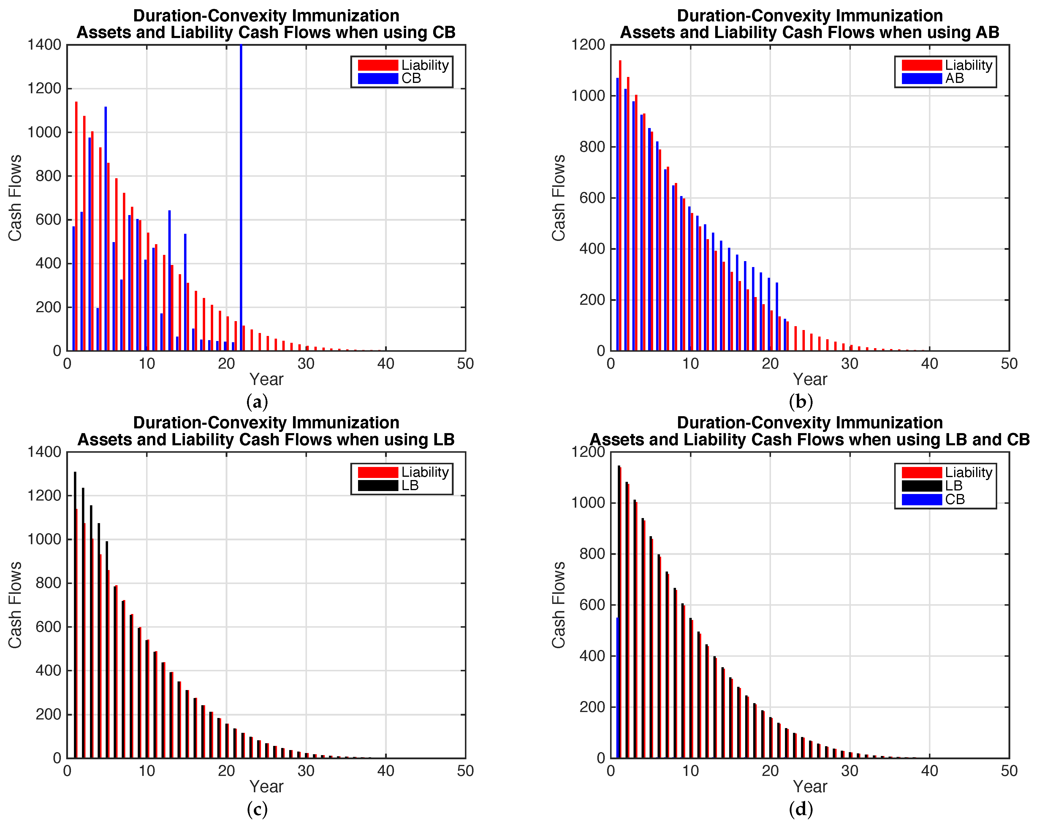
Figure 3 shows the cash flows for the immunized bond portfolios along with the expected liability cash flow. The annuity bonds provide a closer cash flow match than for the coupon bonds. Between years 10 and 20 the cash flows on the annuity bonds exceed the expected liability payments allowing a build up in surplus which is then used to meet the longer term liability cash flows that exceed the term of the longest annuity bonds. The longevity bond portfolio provides an even better cash flow match.
6. Delta-Gamma Hedging
The immunization results using Fisher-Weil dollar duration and convexity considers expected cash flows and the average time to receipt of cash flows incorporating mortality into the discount factor used for valuation. This approach does not explicitly allow for interest rate and mortality rate risks to be separately hedged. A benefit of delta-gamma hedging using sensitivities of the values to interest rates and mortality rates allows explicit recognition of the impact of both interest rate and mortality risks.
We use a linear programming approach with delta and gamma risk factors in order to select bond portfolios that have the same deltas for interest rate and mortality risk as the liability. At the same time we minimize the gamma of the asset portfolio in order to minimize both interest rate and mortality risk. Thne portfolio is determined at time 0 and is a static hedge comparable to the immunization approach.
The linear program used is as follows:
subject to
The bond portfolio is selected to minimize portfolio gamma in Equation (57). The objective used is the sum of the gamma values for each factor multiplied by the factor variances. Equation (60) ensures the surplus is zero initially so that the value f the assets and liabilities match. Since the impact of gamma on the value of the portfolio is multiplied by the factor variance, we weight by the variance. This also gives more weight to the more volatile risk factors. We multiply the objective by to reduce numerical problems with minimizing the objective since it can take small values when multiplied by the variances. This was determined based on the actual numerical size of the objective. The first summation term is for the fixed-income securities and the second summation term is for the longevity bonds, where both interest rate and mortality risk are included.
Equations (58) and (59) ensure the matching of the values of the assets and the liability. Equations (60) to (62) match the deltas of the assets and liabilities. The linear program is formulated in terms of and along with the dollar values of the deltas and gammas. Thus the solution for the and are in terms of units of the bonds based on the price of the bond. This is converted into a percentage of the liability so that the asset portfolio in terms of the proportion of the liability becomes
Equations (63) and (64) express the units of fixed-income assets () and longevity bond assets () as a proportion of the total asset fund ( and ). The proportions invested in all assets are required to sum to 1 so that premiums are fully invested in assets.
Hedge Portfolio Results
Table 13 shows the delta-gamma hedging portfolios of bonds for the different groups of bonds. The interest rate delta of the liability is −2.27 and the interest rate gamma is 5.78. The delta for the first risk factor of mortality, , is −7.79 and the gamma for this factor is 98.20.
For coupon bonds the portfolio selected has 65% in a bond with interest rate delta of −2.15, and interest rate gamma of 4.77, along with 35% in a bond with interest rate delta of −2.50 and interest rate gamma of 6.36. Only two bonds are required for the hedging with only one risk factor to hedge. The hedging is based on the dollar sensitivities so that the relative prices of the bonds and the liability are taken into account in the portfolio.
For the annuity bonds the portfolio selected has 24% in the Waratah annuity bond with monthly cash flows, an interest rate delta of −2.02 and an interest rate gamma of 4.57, along with 76% in the hypothetical annuity bond with quarterly cash flows, a maturity of 21 years, interest rate delta −2.35 and interest rate gamma of 6.08. These are the longest maturity annuity bonds for each of these bond types.
When considering only the longevity bonds, the portfolio requires a short position of 12% of the liability value in the 10 year maturity bond, a short position of 134% in the 20 year longevity bond and long positions in the 5 and 25 year bonds of 22% and 223% respectively. The portfolio requires short selling of longevity bonds to match the liability. This portfolio includes a combination of a short position in the 20 year longevity bond along with a long position in the 25 year longevity bond. This is equivalent to a position in a 20 year deferred, 5 year maturity longevity bond. The selected portfolio has an interest rate delta of −2.27 and an interest rate gamma 5.65. The portfolio delta for the mortality risk factor is −7.79 and the portfolio gamma for this risk factor is 100.35.
When both coupon bonds and annuity bonds are added to the longevity bonds in the portfolio, there is little difference from the case with only longevity bonds. The portfolio consists of a small component of coupon bonds but no additional annuity bonds are included.
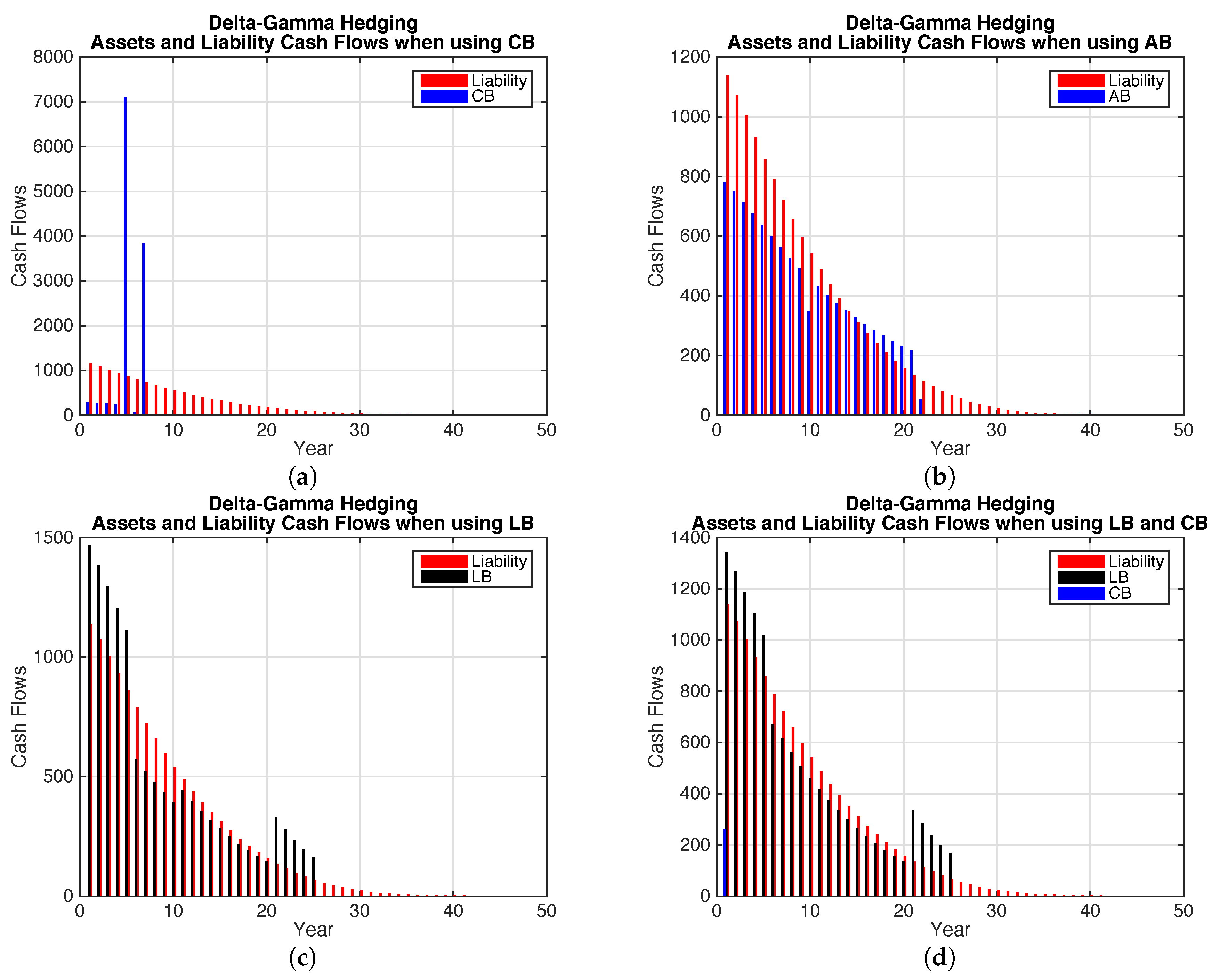
Figure 4 shows the cash flows for the bond portfolios selected with delta-gamma hedging allowing for both mortality and interest rate risk. The coupon bonds have shorter maturities than for the Fisher-Weil duration-convexity immunization portfolio. This reflects the lower sensitivities to maturity for the interest rate deltas for the interest rate risk model.
The liability cash flows are not well matched by the coupon bonds. The annuity bonds provide an improved cash flow match over coupon bonds in a similar way as in the Fisher-Weil duration-convexity immunization. However the liability cash flows exceed the annuity bond cash flows early on and the reverse is the case after the longest maturity annuity bond matures. Including the longevity bonds improves the cash flow match to the liability compared to the coupon and annuity bond cases.
The figures show a similar situation to the immunization case. In general the cash flow match is not as good for the delta-gamma hedge. The delta and gamma values are quite different from the duration and convexity risk measures used in immunization. The result is that for the coupon bonds, the duration of the delta-gamma hedge portfolio is much lower than for the immunization portfolio. However for the longevity bonds, the duration and convexity are much closer to those of the immunization portfolio.
7. Stochastic Assessment of Liability Hedging
Using both traditional immunization and delta-gamma hedging produces differences in the selected bond portfolios. The cash flow match varies depending on which bonds are included in the selected portfolios. In order to assess the differences between the different approaches and resulting portfolios, we use the stochastic interest rate and mortality models to simulate the distribution of the surplus at future time points. This distribution provides a more realistic assessment of the immunization and hedging effectiveness of the different bond portfolios. To do this we generate the surplus at future horizons of 1, 10 and 50 years, the terminal date for the annuity portfolio, to assess the short, medium and long term hedging performance.
7.1. Surplus Analysis
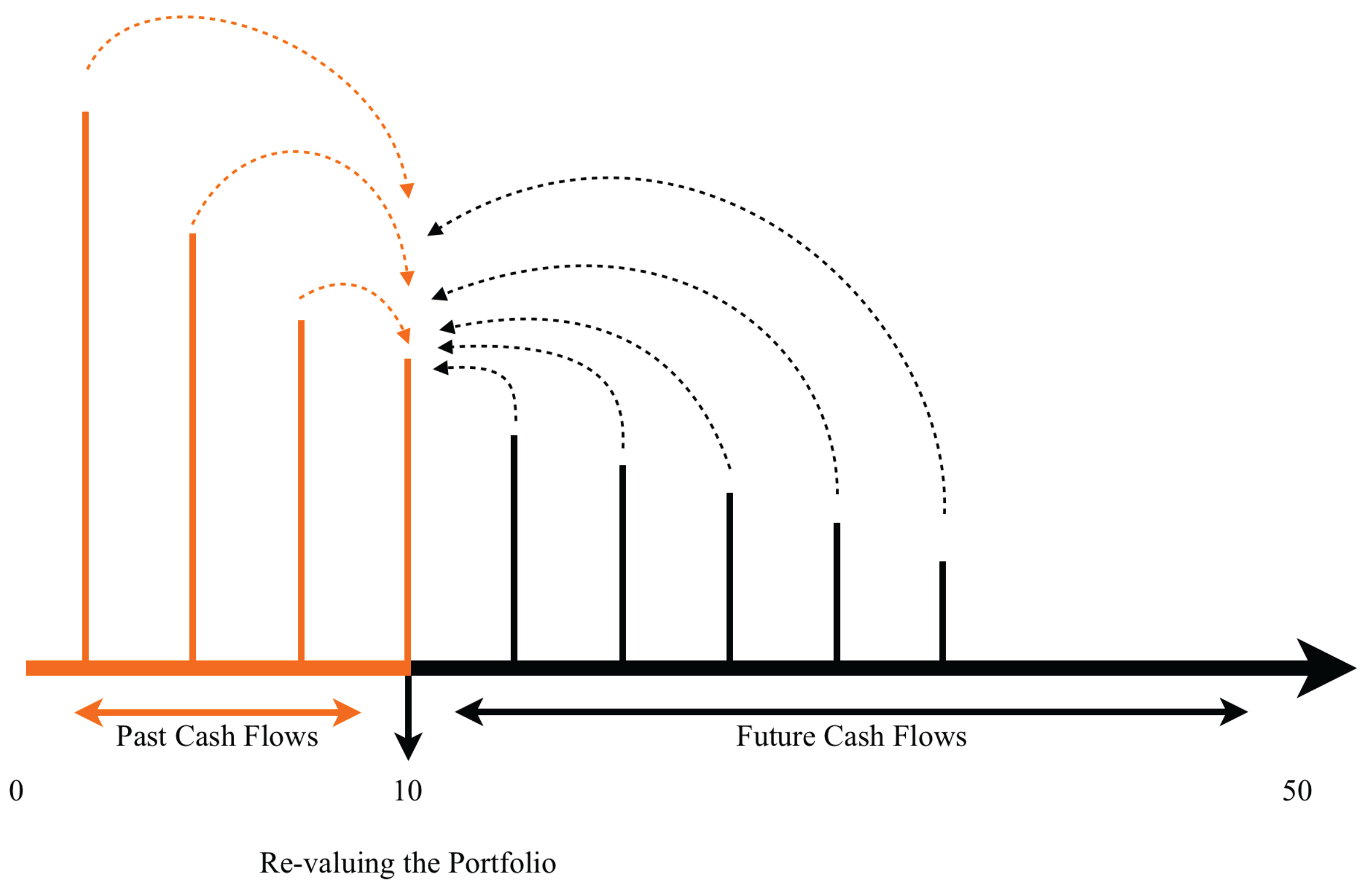
Immunization and hedging strategies require re-balancing of the bond portfolio through time. We allow for this to some extent by assuming reinvestment of cash flows in zero coupon bonds maturing on the horizon date used for the surplus. This reduces the reinvestment risk arising from future interest rates. Figure 5 illustrates the process used to determine the distribution of the surplus for the time horizon of 10 years. Similar calculations are used for the surplus at and 50.
Cash flows prior to the time horizon are accumulated assuming reinvestment in zero-coupon bonds maturing at time 10. All future cash flows occurring after the time horizon are revalued at time 10 using the simulated interest and mortality model values at time 10.
The portfolio surplus at time 10 is determined as the value of the assets minus the value of the liabilities:
where and are the number of units of fixed-income and longevity-linked bonds respectively. The portfolio surplus is thus the sum of the net accumulated cash flows and the net expected value of the future cash flows at time 10.
These values for the fixed-income assets (k), longevity-linked assets (j), and annuity liability at time 10 are determined using:
where for ,
is the zero-coupon bond price at time t maturing at time 10 and is the simulated interest rate at time t, and for ,
is the zero-coupon bond price at time maturing at time t and is the simulated interest rate at time 10.
For , and are the simulated survival probabilities, and for ,
is the projected survival probability at time 10 for age over years. and are the simulated mortality factors at time 10.
Figure 6 gives plots of the surplus for the different time horizons for the immunization portfolios. Each sub-figure shows a comparison of the surplus distribution for the different immunized bond portfolios. The improvement in the surplus distribution when longevity bonds are included is dramatic regardless of the time horizon. There is little difference between the coupon and annuity bonds. Although the annuity bonds appear to provide a better cash flow match, there is little difference in the surplus distribution. The annuity bonds do require fewer bonds to be held compared to coupon bonds.
Table 14 gives summary statistics for the surplus distributions showing the mean, standard deviation, value at risk () and expected shortfall () at the 0.5% probability level for the immunization portfolios. is a quantile measure that represents the worst expected loss over the given time period at confidence level α and Expected Shortfall () reflects the losses in the tail of the distribution. The confidence level used reflects the Solvency II risk levels of 1 in 200. These are expressed as a percentage of the initial liability value.
The mean surplus is approximately zero as expected. All the risk measures demonstrate the improvement from including longevity bonds in the portfolio. Even if interest rate risk is immunized, the 1 in 200 loss could be as high as 10% over a 10 year horizon and 10% over the full time horizon for the life annuity. Longevity bonds allow this risk to be reduced to less than 0.5% over a 10 year horizon and less than 0.6% over the full time horizon.
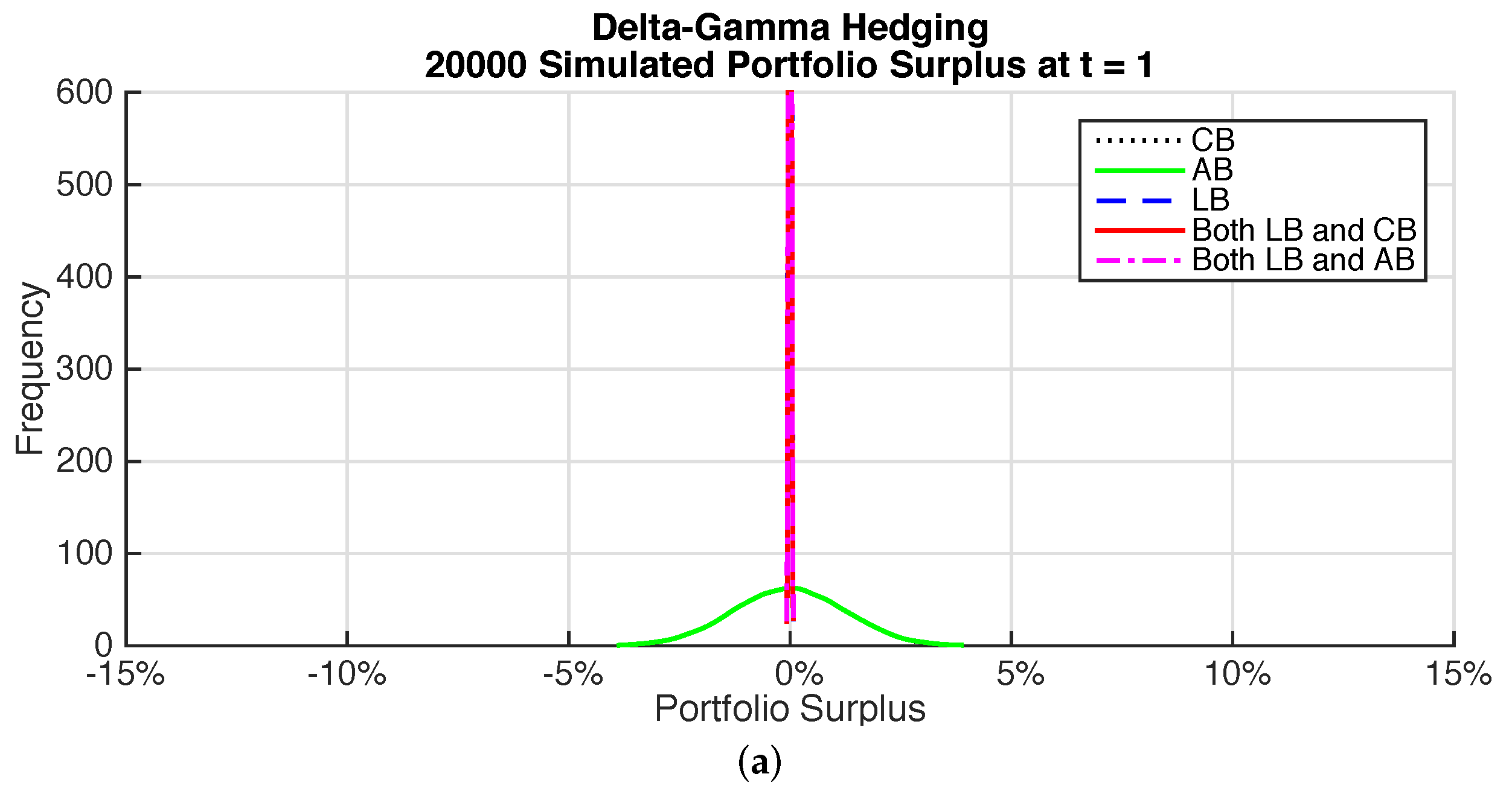
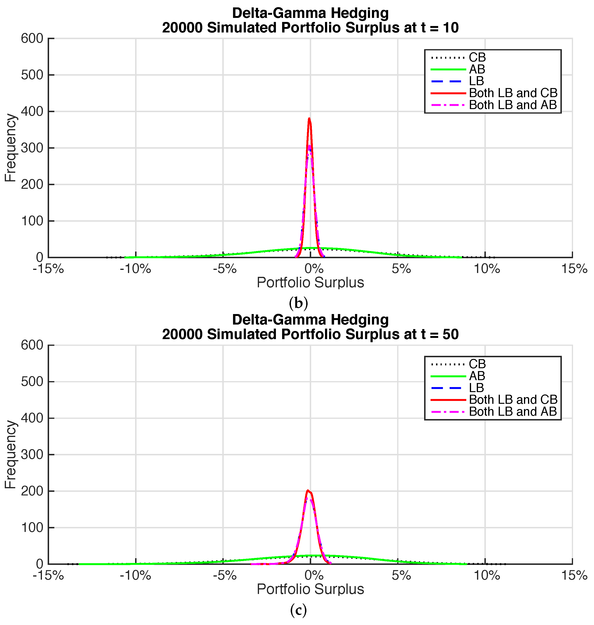
Figure 7 shows plots of the surplus for the varying time horizons for the different delta-gamma hedged bond portfolios. The benefits of holding longevity bonds are again very noticeable with significant reductions in the variability in surplus over all horizons compared to portfolios without longevity bonds. Although results are broadly similar to those for the immunization portfolios there are some noticeable differences. The coupon bond portfolio has more variability than the annuity bond portfolio over medium and long horizons. The portfolios that include longevity bonds have more variability than for the immunized portfolios.
Table 15 gives summary statistics for the surplus distributions for the delta-gamma hedging. For the coupon and annuity bond portfolios the risk measures are relatively large for all horizons.
All of the risk measures show significant reductions when longevity bonds are included. These reductions are not as great for the long horizon of 50 years compared to the short and medium term horizons.
There is very little difference when coupon bonds and annuity bonds are included in the portfolio along with the longevity bonds, as compared to including only longevity bonds.
7.2. Portfolio Hedge Effectiveness
Although there are clear benefits demonstrated from holding longevity bonds, in order to assess the significance of this improvement we consider three measures of the relative hedge effectiveness of the different portfolios. They are the standard deviation reduction ratio used in Lin and Tsai [7], the Value at Risk reduction ratio , and the expected shortfall reduction ratio used in Ngai and Sherris [21]. These measures are defined in Table 16.
To interpret the risk reduction measures, a negative figure indicates the former strategy with surplus performs better than the latter strategy with surplus and vice versa.
Table 17 shows the risk reductions at , and . Annuity bonds provide improved hedging compared to coupon bonds, especially over longer horizons.
Longevity bonds produce significant risk reductions regardless of the horizon used for the surplus when compared to using only coupon bonds. The reduction is almost complete and highlights the significance of longevity risk in life annuity portfolios that cannot be immunized or hedged with fixed-income securities. The reduction is not as great over the longer horizon when using delta-gamma hedging. Longevity bonds provide better match to the underlying liability and as a result provide the most effective immunization of the life annuity liability.
Table 18 compares the risk reductions for delta-gamma hedging portfolios with the immunization portfolios. For the coupon portfolios, immunization is more effective in risk reduction than is delta-gamma hedging. For annuity bonds there is little difference between the two approaches regardless of the horizon used.
For the longevity bonds, delta-gamma hedging portfolios are more effective over shorter horizons than immunization but significantly worse in effectiveness over medium and longer horizons. The combination of short and long positions in the longevity bonds with delta-gamma hedging is only more effective over short horizons.
Including coupon bonds along with longevity bonds produces delta-gamma hedging portfolios that are considerably less effective than the immunized portfolios. This reflects the inclusion of short positions in the delta-gamma longevity bond portfolios that resemble deferred longevity bonds. Since these are selected to hedge the delta and gamma, based on the stochastic model used, they do not provide the cash flow hedge that immunization does.
8. Conclusions
This paper presents an extensive analysis of bond portfolio selection for immunizing and hedging the life annuity liabilities of a life annuity provider. The paper assesses both Fisher-Weil immunization as well as delta-gamma hedging using stochastic models for both interest rate risk and mortality risk. The portfolios considered include coupon bonds, annuity bonds and longevity bonds.
We show how Fisher-Weil immunization can be used to immunize both interest rate and mortality risk. We extend a linear-programming approach used for interest rate immunization to selecting coupon, annuity and longevity bonds to immunize a life annuity portfolio. We use a linear programming approach for delta-gamma hedging and allow for both interest rate and mortality risk.
We show that annuity bonds provide better cash flow matching than coupon bonds, although the annuity bonds available in the Australian market do not have a long enough term to maturity to immunize a life annuity portfolio. Annuity bonds provide a better cash flow match to the life annuity liability, with improved immunization effectiveness compared with coupon bonds over short horizons.
For the delta-gamma hedging portfolio with longevity bonds, a short position in a shorter term bond and a long position in a longer term bond is required. This is the equivalent of a deferred longevity bond. Although this portfolio performs well over the short horizon, it does not perform well compared to the immunized portfolio over medium or long horizons.
The portfolios selected, regardless of method, all demonstrate that longevity bonds are extremely valuable in immunizing or hedging longevity risk in life annuities. They provide a better cash flow match in the case of immunization and have much reduced risk in the surplus distribution at short, medium and long horizons.
Longevity bonds are not available in the Australian market or in other bond markets. We have shown the clear benefits that these bonds bring to the risk management of a life annuity provider. As a result we expect that as the life annuity market develops these bonds should be in increasing demand by insurers.
Our analysis uses Australia bonds as well as stochastic models calibrated to Australian interest rate and mortality data. Most developed economies have similar bond markets as well as interest rate and mortality experience as has Australia. As a result our analysis has direct application to any economy considering the types of bonds that should be offered in order to better manage the risks of long term pension and annuity portfolios.
Acknowledgments
The authors acknowledge financial support from the CEPAR Honours Scholarship, the EJ Blackadder Honours Scholarship, the CIFR Honours Scholarship and support from the Australian Research Council Centre of Excellence in Population Ageing Research (project number CE110001029).
Author Contributions
Changyu Liu and Michael Sherris jointly designed and develoed the research project and jointly worte the paper. Changyu Liu carried out the computation.
Conflicts of Interest
The authors declare no conflict of interest.
References
- F.M. Redington. “Review of the principles of life-office valuations.” J. Inst. Actuar. 78 (1952): 286–340. [Google Scholar]
- L. Fisher, and R.L. Weil. “Coping with the risk of interest-rate fluctuations: Returns to bondholders from naive and optimal strategies.” J. Bus. 44 (1971): 408–431. [Google Scholar] [CrossRef]
- E.S. Shiu. “On the fisher-weil immunization theorem.” Insur.: Math. Econ. 6 (1987): 259–266. [Google Scholar] [CrossRef]
- E.S. Shiu. “Immunization of multiple liabilities.” Insur.: Math. Econ. 7 (1988): 219–224. [Google Scholar] [CrossRef]
- E.S. Shiu. “On Redington’s theory of immunization.” Insur.: Math. Econ. 9 (1990): 171–175. [Google Scholar] [CrossRef]
- C.C.-L. Tsai, and S.-L. Chung. “Actuarial applications of the linear hazard transform in mortality immunization.” Insur.: Math. Econ. 53 (2013): 48–63. [Google Scholar] [CrossRef]
- T. Lin, and C.C.-L. Tsai. “On the mortality/longevity risk hedging with mortality immunization.” Insur.: Math. Econ. 53 (2013): 580–596. [Google Scholar] [CrossRef]
- E. Luciano, L. Regis, and E. Vigna. “Delta–gamma hedging of mortality and interest rate risk.” Insur.: Math. Econ. 50 (2012): 402–412. [Google Scholar] [CrossRef]
- D.F. Schrager. “Affine stochastic mortality.” Insur.: Math. Econ. 38 (2006): 81–97. [Google Scholar] [CrossRef]
- E. Biffis. “Affine processes for dynamic mortality and actuarial valuations.” Insur.: Math. Econ. 37 (2005): 443–468. [Google Scholar] [CrossRef]
- C. Blackburn, and M. Sherris. “Consistent dynamic affine mortality models for longevity risk applications.” Insur.: Math. Econ. 53 (2013): 64–73. [Google Scholar] [CrossRef]
- A. Wong, M. Sherris, and R. Stevens. “Natural Hedging Strategies for Life Insurers: Impact of Product Design and Risk Measure.” J. Risk Insurance 84 (2017): 153–175. [Google Scholar]
- Human Mortality Database. “University of California, Berkeley (USA), and Max Planck Institute for Demographic Research (Germany).” Available online: www.mortality.org (accessed on 10 June 2014).
- S.J. Koopman, and J. Durbin. “Fast filtering and smoothing for multivariate state space models.” J. Time Ser. Anal. 21 (2000): 281–296. [Google Scholar] [CrossRef]
- J.C. Cox, J.E. Ingersoll Jr., and S.A. Ross. “A theory of the term structure of interest rates.” Econometrica 53 (1985): 385–408. [Google Scholar] [CrossRef]
- L.C. Rogers, and W. Stummer. “Consistent fitting of one-factor models to interest rate data.” Insur.: Math. Econ. 27 (2000): 45–63. [Google Scholar] [CrossRef]
- K. Kladıvko. Maximum Likelihood Estimation of the Cox-Ingersoll-Ross Process: The Matlab Implementation. Praha, Czech Republic: Technical Computing Prague, 2007. [Google Scholar]
- L. Mátyás. Generalized Method of Moments Estimation. Cambridge, UK: Cambridge University Press, 1999, Volume 5. [Google Scholar]
- H.H. Panjer, P.P. Boyle, S.H. Cox, D. Dufresne, H.U. Gerber, H.H. Mueller, H.W. Pedersen, S.R. Pliska, M. Sherris, E. Shiu, and et al. Financial Economics: With Applications to Investments, Insurance, and Pensions. Schaumburg, IL, USA: Society of Actuaries Foundation, 1997. [Google Scholar]
- F. Menoncin. “The role of longevity bonds in optimal portfolios.” Insur.: Math. Econ. 42 (2008): 343–358. [Google Scholar] [CrossRef]
- A. Ngai, and M. Sherris. “Longevity risk management for life and variable annuities: The effectiveness of static hedging using longevity bonds and derivatives.” Insur.: Math. Econ. 49 (2011): 100–114. [Google Scholar] [CrossRef]
Figure 1.
Historical (1960–2009) and Projected (2010–2050) Mortality Rates for Australian Population Males Aged 50–100.
Figure 1.
Historical (1960–2009) and Projected (2010–2050) Mortality Rates for Australian Population Males Aged 50–100.

Figure 2.
Yield Curve for 50 years as at 30 June 2014.
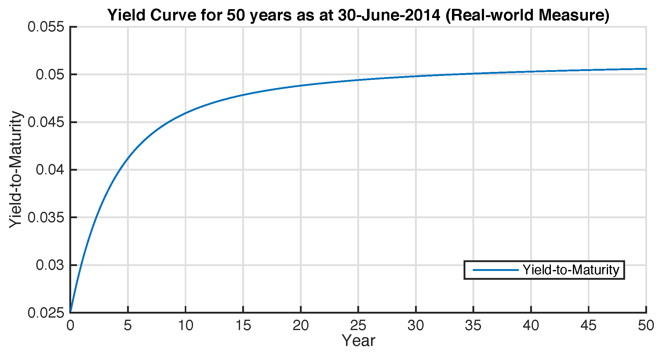
Figure 3.
Asset and Liability Cash Flows—Immunization. (a) Only Coupon Bonds; (b) Only Annuity Bonds; (c) Only Longevity Bonds; (d) Coupon Bonds and Longevity Bonds; (e) Annuity Bonds and Longevity Bonds.
Figure 3.
Asset and Liability Cash Flows—Immunization. (a) Only Coupon Bonds; (b) Only Annuity Bonds; (c) Only Longevity Bonds; (d) Coupon Bonds and Longevity Bonds; (e) Annuity Bonds and Longevity Bonds.

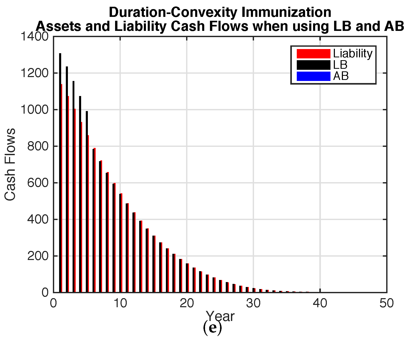
Figure 4.
Asset and Liability Cash Flows—Hedging. (a) Only Coupon Bonds; (b) Only Annuity Bonds; (c) Only Longevity Bonds; (d) Coupon Bonds and Longevity Bonds; (e) Coupon Bonds and Longevity Bonds.
Figure 4.
Asset and Liability Cash Flows—Hedging. (a) Only Coupon Bonds; (b) Only Annuity Bonds; (c) Only Longevity Bonds; (d) Coupon Bonds and Longevity Bonds; (e) Coupon Bonds and Longevity Bonds.

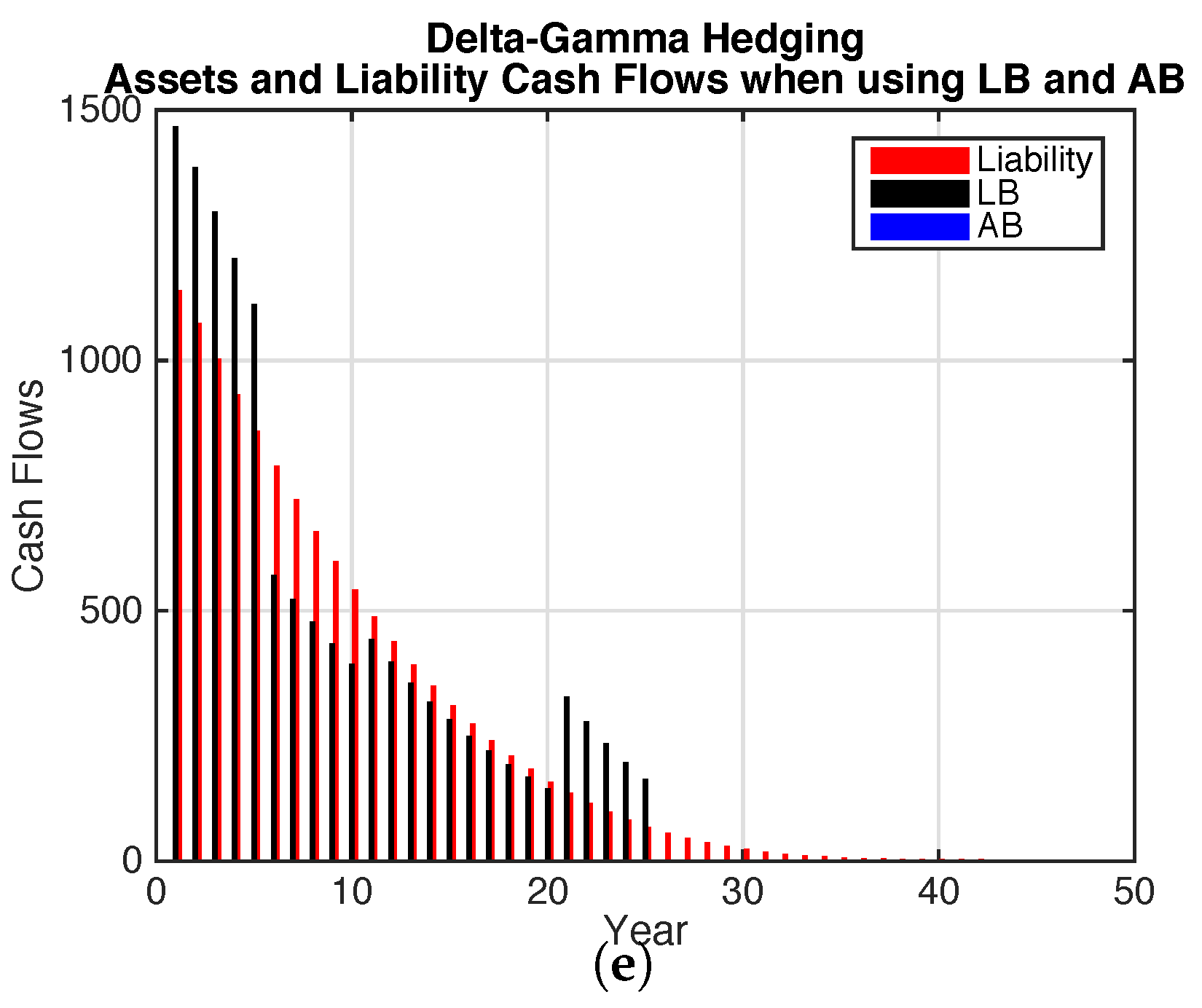
Figure 5.
Illustration of Simulation for the Portfolio Surplus.

Figure 6.
Surplus Distribution—Immunization. (a) Time horizon—1 year; (b) Time horizon—10 years; (c) Time horizon—50 years.
Figure 6.
Surplus Distribution—Immunization. (a) Time horizon—1 year; (b) Time horizon—10 years; (c) Time horizon—50 years.
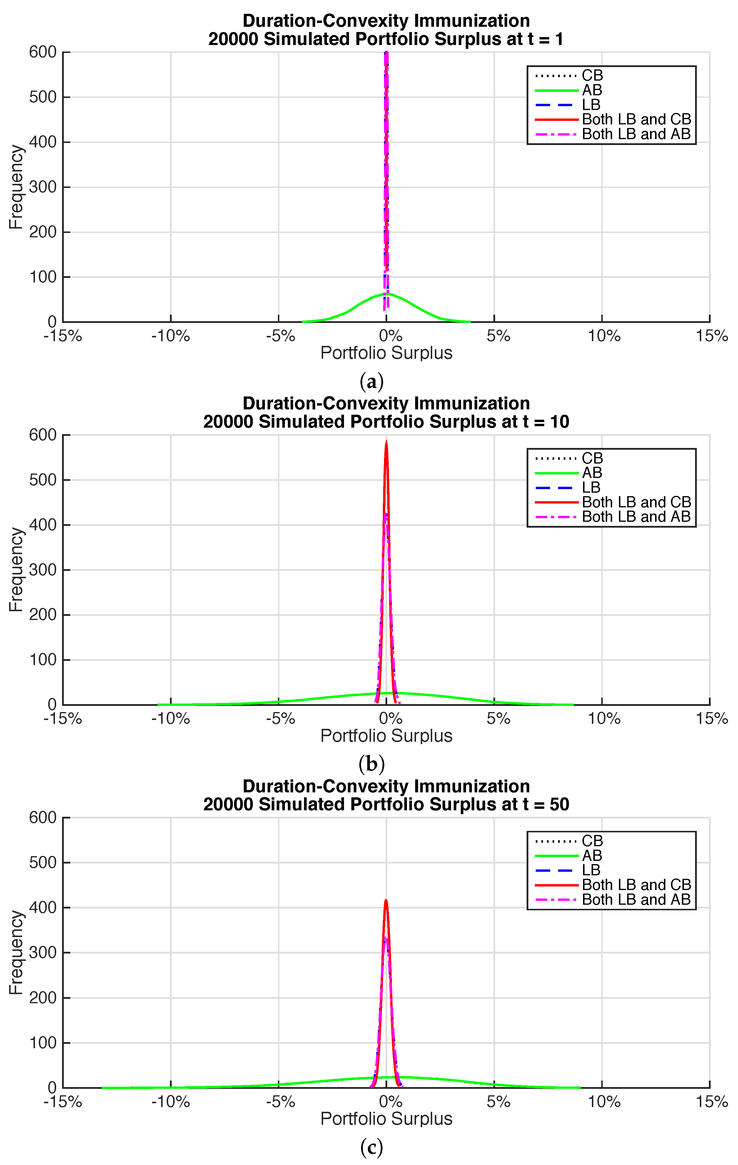
Figure 7.
Surplus Distribution—Delta-Gamma hedging. (a) Time horizon—1 year; (b) Time horizon—10 years; (c) Time horizon—50 years.
Figure 7.
Surplus Distribution—Delta-Gamma hedging. (a) Time horizon—1 year; (b) Time horizon—10 years; (c) Time horizon—50 years.


Table 1.
Parameters of the Calibrated Mortality Model—Australian Population Males Aged 50 to 100 for years 1960 to 2009.
| Parameter | Estimate | Standard Error |
|---|---|---|
| 0.00621 | 1.48e-04 | |
| 0.000742 | 1.93e-05 | |
| 0.000204 | 5.92e-07 | |
| 0.0000148 | 7.79e-09 | |
| c | 1.092 | 6.19e-06 |
Table 2.
Parameters of the Calibrated Interest Rate Model—Australian Interest Rate Data 4 January 1993 to 31 July 2014.
| Parameter 1 | Estimate | Standard Error |
|---|---|---|
| 0.445 | 0.0022 | |
| 0.0523 | 0.0012 | |
| 0.0414 | 0.0013 | |
| −0.111 | 0.0022 |
and are parameters under measure.
| Fixed-Income Securities (k) | Longevity-Linked Securities (j) | Liabilities |
|---|---|---|
| Fixed-Income Securities (k) | Longevity-Linked Securities (j) | Liabilities |
|---|---|---|
| - | ||
| - | ||
| - | ||
| - |
Table 6.
These are details of the life annuity with monthly payments. The deltas with respect to the mortality risk factors are negative. Increases in these factors produce lower survival probabilities used for the discount factors and hence lower annuity values. The interest rate delta is also negative. Increases in the short rate produce lower zero coupon bond prices and hence lower annuity values. For a 65 year old, the Fisher-Weil duration is 8.12 years. Interest rate sensitivity for the stochastic interest rate model is lower than the Fisher-Weil duration. The delta for the mortality risk factor is of a similar magnitude as the duration, with opposite sign. reflects the level of mortality, whereas captures the impact of age.
| Code | Maturity | TTM | Freq | Price | ||||||||
|---|---|---|---|---|---|---|---|---|---|---|---|---|
| IA-WL | ∞ | ∞ | 12 | 127.67 | −7.79 | −5.08E+03 | −2.27 | 98.20 | 7.85E+07 | 5.78 | 8.12 | 109.23 |
Table 7.
These are semi-annual coupon paying bonds available in the bond market. Codes used are those for the ASX. Maturities range up to 18.8 years and Fisher-Weil durations range up to 11.82 years with the longest duration exceeding that of the life annuity. The interest rate deltas range up to 2.62 and are all similar for bonds maturing longer than 4 years. Fisher-Weil convexity varies much more than interest rate gamma across the maturity range of the bonds.
| Code | Sector | Coupon | Maturity | TTM | FV | Freq | Price | ||||
|---|---|---|---|---|---|---|---|---|---|---|---|
| GSBS-CB-14 | Government | 4.50 % | 21/10/2014 | 0.31 | 100 | 2 | 101.39 | −0.29 | 0.09 | 0.31 | 0.10 |
| GSBS-CB-15 | Government | 4.75 % | 21/10/2015 | 1.31 | 100 | 2 | 102.65 | −1.03 | 1.08 | 1.28 | 1.65 |
| GSBM-CB-17 | Government | 4.25 % | 21/07/2017 | 3.06 | 100 | 2 | 102.05 | −1.79 | 3.35 | 2.85 | 8.53 |
| GSBA-CB-18 | Government | 5.50 % | 21/01/2018 | 3.56 | 100 | 2 | 106.13 | −1.90 | 3.83 | 3.21 | 11.10 |
| GSBS-CB-18 | Government | 3.25 % | 21/10/2018 | 4.31 | 100 | 2 | 95.33 | −2.15 | 4.77 | 4.02 | 16.93 |
| GSBG-CB-23 | Government | 5.50 % | 21/04/2023 | 8.81 | 100 | 2 | 101.44 | −2.47 | 6.49 | 6.99 | 56.56 |
| GSBG-CB-24 | Government | 2.75 % | 21/04/2024 | 9.82 | 100 | 2 | 79.06 | −2.62 | 7.16 | 8.39 | 77.99 |
| GSBG-CB-25 | Government | 3.25 % | 21/04/2025 | 10.82 | 100 | 2 | 80.99 | −2.60 | 7.13 | 8.85 | 89.19 |
| GSBG-CB-26 | Government | 4.25 % | 21/04/2026 | 11.82 | 100 | 2 | 88.01 | −2.56 | 6.97 | 9.04 | 96.85 |
| GSBG-CB-27 | Government | 4.75 % | 21/04/2027 | 12.82 | 100 | 2 | 91.41 | −2.54 | 6.91 | 9.35 | 106.67 |
| GSBG-CB-29 | Government | 3.25 % | 21/04/2029 | 14.82 | 100 | 2 | 74.11 | −2.61 | 7.22 | 11.04 | 147.40 |
| GSBG-CB-33 | Government | 4.50 % | 21/04/2033 | 18.82 | 100 | 2 | 83.37 | −2.55 | 6.94 | 11.82 | 186.06 |
| GSBG-CB-15 | Government | 6.25 % | 15/04/2015 | 0.79 | 100 | 2 | 103.77 | −0.68 | 0.47 | 0.78 | 0.61 |
| GSBK-CB-16 | Government | 4.75 % | 15/06/2016 | 1.96 | 100 | 2 | 102.13 | −1.39 | 1.97 | 1.89 | 3.66 |
| GSBC-CB-17 | Government | 6.00 % | 15/02/2017 | 2.63 | 100 | 2 | 107.13 | −1.63 | 2.77 | 2.43 | 6.23 |
| GSBE-CB-19 | Government | 5.25 % | 15/03/2019 | 4.71 | 100 | 2 | 103.81 | −2.15 | 4.88 | 4.17 | 18.85 |
| GSBG-CB-20 | Government | 4.50 % | 15/04/2020 | 5.80 | 100 | 2 | 98.56 | −2.33 | 5.68 | 5.10 | 28.25 |
| GSBI-CB-21 | Government | 5.75 % | 15/05/2021 | 6.88 | 100 | 2 | 104.08 | −2.38 | 6.01 | 5.74 | 36.91 |
| GSBM-CB-22 | Government | 5.75 % | 15/07/2022 | 8.05 | 100 | 2 | 105.28 | −2.40 | 6.22 | 6.38 | 47.39 |
Table 8.
These are hypothetical coupon paying bonds with coupons and maturities corresponding to index linked bonds available on the FIIG web site. We do not include inflation in the analysis so we have used these as hypothetical coupon paying bonds with quarterly frequency. These hypothetical bonds have longer duration compared to the Government Coupon bonds. They also have quarterly coupon cash flows.
| Code | Sector | Coupon | Maturity | TTM | FV | Freq | Price | ||||
|---|---|---|---|---|---|---|---|---|---|---|---|
| ACG-CB-15 | Government | 4.00 % | 20/08/2015 | 1.14 | 100 | 4 | 101.26 | −0.93 | 0.87 | 1.12 | 1.26 |
| ACG-CB-20 | Government | 4.00 % | 20/08/2020 | 6.15 | 100 | 4 | 95.06 | −2.38 | 5.91 | 5.42 | 31.87 |
| ACG-CB-22 | Government | 1.25 % | 21/02/2022 | 7.65 | 100 | 4 | 74.54 | −2.63 | 7.08 | 7.21 | 54.15 |
| ACG-CB-25 | Government | 3.00 % | 20/09/2025 | 11.23 | 100 | 4 | 77.73 | −2.63 | 7.23 | 9.22 | 96.65 |
| ACG-CB-30 | Government | 2.50 % | 20/09/2030 | 16.24 | 100 | 4 | 63.77 | −2.65 | 7.40 | 12.31 | 181.46 |
| SAFA-CB-15 | Semi-govern | 4.00 % | 20/08/2015 | 1.14 | 100 | 4 | 101.26 | −0.93 | 0.87 | 1.12 | 1.26 |
| TCV-CB-20 | Semi-govern | 4.00 % | 15/08/2020 | 6.13 | 100 | 4 | 95.13 | −2.37 | 5.90 | 5.40 | 31.72 |
| ACT-CB-30 | Semi-govern | 3.50 % | 17/06/2030 | 15.98 | 100 | 4 | 74.83 | −2.60 | 7.16 | 11.41 | 161.28 |
| QTC-CB-30 | Semi-govern | 2.75 % | 20/08/2030 | 16.15 | 100 | 4 | 66.80 | −2.63 | 7.31 | 12.01 | 174.92 |
| NSWTC-CB-20 | Semi-govern | 3.75 % | 20/11/2020 | 6.40 | 100 | 4 | 93.20 | −2.41 | 6.07 | 5.65 | 34.59 |
| NSWTC-CB-25 | Semi-govern | 2.75 % | 20/11/2025 | 11.40 | 100 | 4 | 75.47 | −2.63 | 7.28 | 9.41 | 100.52 |
| NSWTC-CB-35 | Semi-govern | 2.50 % | 20/11/2035 | 21.41 | 100 | 4 | 56.85 | −2.61 | 7.25 | 14.30 | 265.62 |
| ELECTRANET-CB-15 | Infrastructure | 5.21 % | 20/08/2015 | 1.14 | 100 | 4 | 102.74 | −0.92 | 0.86 | 1.11 | 1.25 |
| LANECOVE-CB-20 | Infrastructure | 4.50 % | 9/09/2020 | 6.20 | 100 | 4 | 97.46 | −2.37 | 5.88 | 5.40 | 31.89 |
| SYDAIR-CB-20 | Infrastructure | 3.76 % | 20/11/2020 | 6.40 | 100 | 4 | 93.25 | −2.41 | 6.07 | 5.64 | 34.58 |
| SYDAIR-CB-30 | Infrastructure | 3.12 % | 20/11/2030 | 16.40 | 100 | 4 | 70.42 | −2.61 | 7.21 | 11.82 | 172.67 |
| RABO-CB-20 | ADI-IB | 1.51 % | 28/08/2020 | 6.17 | 100 | 4 | 81.37 | −2.50 | 6.36 | 5.85 | 35.42 |
| CBA-CB-20 | ADI-Major Bank | 3.60 % | 20/11/2020 | 6.40 | 100 | 4 | 92.35 | −2.41 | 6.09 | 5.67 | 34.79 |
| ALE-CB-23 | Other Financials | 3.40 % | 20/11/2023 | 9.40 | 100 | 4 | 84.89 | −2.57 | 6.94 | 7.86 | 69.45 |
| ENVESTRA-CB-25 | Energy | 3.04 % | 20/08/2025 | 11.15 | 100 | 4 | 78.49 | −2.61 | 7.19 | 9.12 | 94.87 |
Table 9.
These are annuity bonds with monthly payments. Terms to maturity are relatively short compared to the coupon paying bonds with a maximum of around 9 years. Fisher-Weil durations are between 3 and 5 years. Interest rate deltas do not vary much. Similar comments apply to interest rate gamma and Fisher-Weil convexity. Since the life annuity is assumed to have monthly payments these annuity bonds have the potential to better match the cash flows for the liability but suffer from having short maturities.
| Code | Sector | Annuity Payment | Maturity | TTM | Freq | No. of Payment | Price | ||||
|---|---|---|---|---|---|---|---|---|---|---|---|
| NSWWAB1-AB-21 | Semi-govern | 1.00 | 15/10/2021 | 7.30 | 12 | 111 | 74.60 | −1.79 | 3.77 | 3.43 | 16.17 |
| NSWWAB2-AB-21 | Semi-govern | 1.00 | 15/10/2021 | 7.30 | 12 | 108 | 74.60 | −1.79 | 3.77 | 3.43 | 16.17 |
| NSWWAB3-AB-22 | Semi-govern | 1.00 | 15/01/2022 | 7.55 | 12 | 108 | 76.62 | −1.81 | 3.86 | 3.54 | 17.22 |
| NSWWAB4-AB-22 | Semi-govern | 1.00 | 15/04/2022 | 7.80 | 12 | 108 | 78.60 | −1.83 | 3.95 | 3.64 | 18.28 |
| NSWWAB5-AB-22 | Semi-govern | 1.00 | 15/07/2022 | 8.05 | 12 | 108 | 80.56 | −1.86 | 4.04 | 3.75 | 19.38 |
| NSWWAB6-AB-22 | Semi-govern | 1.00 | 15/10/2022 | 8.30 | 12 | 108 | 82.48 | −1.88 | 4.13 | 3.85 | 20.50 |
| NSWWAB7-AB-23 | Semi-govern | 1.00 | 15/01/2023 | 8.55 | 12 | 108 | 84.36 | −1.90 | 4.21 | 3.95 | 21.64 |
| NSWWAB8-AB-23 | Semi-govern | 1.00 | 15/04/2023 | 8.80 | 12 | 108 | 86.22 | −1.92 | 4.29 | 4.06 | 22.81 |
| NSWWAB9-AB-23 | Semi-govern | 1.00 | 15/07/2023 | 9.05 | 12 | 108 | 87.05 | −1.96 | 4.41 | 4.20 | 24.28 |
| NSWWAB10-AB-23 | Semi-govern | 1.00 | 15/07/2023 | 9.05 | 12 | 105 | 84.06 | −2.02 | 4.57 | 4.35 | 25.14 |
Table 10.
These are hypothetical annuity bonds with maturities corresponding to index linked bonds available on FIIG. We do not include inflation in the analysis so we have used these as hypothetical annuity bonds with quarterly frequency. Terms to maturity are longer than for the Waratah annuity bonds. We do not adjust pricing for credit risk.
| Code | Sector | Annuity Payment | Maturity | TTM | Freq | No. of Payment | Price | ||||
|---|---|---|---|---|---|---|---|---|---|---|---|
| MPC-AB-25 | Infrastructure | 1.00 | 31/12/2025 | 11.51 | 4 | 46 | 34.49 | −2.11 | 5.05 | 5.23 | 37.95 |
| MPC-AB-33 | Infrastructure | 1.00 | 31/12/2033 | 19.52 | 4 | 78 | 46.99 | −2.33 | 5.99 | 7.90 | 91.30 |
| CIVICNEXUS-AB-32 | Infrastructure | 1.00 | 15/09/2032 | 18.22 | 4 | 73 | 45.57 | −2.30 | 5.87 | 7.48 | 81.61 |
| PHF-AB-29 | Other Financials | 1.00 | 15/09/2029 | 15.22 | 4 | 61 | 41.31 | −2.23 | 5.58 | 6.52 | 60.83 |
| PJS-AB-30 | Other Financials | 1.00 | 15/06/2030 | 15.97 | 4 | 64 | 42.46 | −2.25 | 5.67 | 6.77 | 65.88 |
| Novacare-AB-33 | Other Financials | 1.00 | 15/04/2033 | 18.81 | 4 | 76 | 46.97 | −2.28 | 5.83 | 7.55 | 84.60 |
| Praeco-AB-20 | Other Corporate | 1.00 | 15/08/2020 | 6.13 | 4 | 25 | 21.82 | −1.66 | 3.31 | 2.96 | 11.98 |
| Boral-AB-20 | Other Corporate | 1.00 | 16/11/2020 | 6.39 | 4 | 26 | 22.54 | −1.70 | 3.43 | 3.07 | 12.92 |
| WYUNA-AB-22 | Other Corporate | 1.00 | 30/03/2022 | 7.75 | 4 | 31 | 12.58 | −1.84 | 3.95 | 3.61 | 17.69 |
| JEM(CCV)-AB-22 | Other Corporate | 1.00 | 15/06/2022 | 7.96 | 4 | 32 | 26.52 | −1.88 | 4.09 | 3.79 | 19.62 |
| JEM-AB-35 | Other Corporate | 1.00 | 28/06/2035 | 21.01 | 4 | 84 | 48.67 | −2.35 | 6.08 | 8.32 | 102.30 |
| JEM(NSWSch)-AB-31 | Other Corporate | 1.00 | 28/02/2031 | 16.68 | 4 | 67 | 43.66 | −2.26 | 5.72 | 6.98 | 70.48 |
| JEM(NSWSch)-AB-35 | Other Corporate | 1.00 | 28/11/2035 | 21.43 | 4 | 86 | 49.44 | −2.34 | 6.06 | 8.38 | 104.73 |
| ANU-AB-29 | Other Corporate | 1.00 | 7/10/2029 | 15.28 | 4 | 62 | 42.16 | −2.20 | 5.49 | 6.43 | 60.14 |
Table 11.
These longevity bonds are hypothetical bonds with maturities at 5 year intervals up to a maximum of 50 years. They are based on a cohort aged 65 at issue. Fisher-Weil durations at the longer maturities do not vary much with a maximum of 8.48 years. The interest rate deltas also show very little variation with maturity. The deltas for in the mortality model are of a similar magnitude to the Fisher-Weil durations. The gammas for are of a similar magnitude to the convexity. The deltas for the are larger and reflect the impact of age.
| Code | Maturity | TTM | Freq | Price | ||||||||
|---|---|---|---|---|---|---|---|---|---|---|---|---|
| LB65-19 | 30/06/2019 | 5 | 1 | 420.94 | −2.83 | −1.00E+03 | −1.71 | 9.92 | 1.31E+06 | 3.23 | 2.86 | 10.17 |
| LB65-24 | 30/06/2024 | 10 | 1 | 699.86 | −4.74 | −1.96E+03 | −2.11 | 29.81 | 5.66E+06 | 4.89 | 4.83 | 31.23 |
| LB65-29 | 30/06/2029 | 15 | 1 | 866.81 | −6.19 | −2.94E+03 | −2.26 | 53.41 | 1.45E+07 | 5.58 | 6.36 | 57.03 |
| LB65-34 | 30/06/2034 | 20 | 1 | 956.71 | −7.18 | −3.86E+03 | −2.33 | 74.98 | 2.88E+07 | 5.87 | 7.43 | 81.38 |
| LB65-39 | 30/06/2039 | 25 | 1 | 998.30 | −7.77 | −4.59E+03 | −2.35 | 90.50 | 4.70E+07 | 5.98 | 8.07 | 99.45 |
| LB65-44 | 30/06/2044 | 30 | 1 | 1,013.60 | −8.03 | −5.05E+03 | −2.36 | 98.84 | 6.47E+07 | 6.03 | 8.36 | 109.46 |
| LB65-49 | 30/06/2049 | 35 | 1 | 1,017.70 | −8.12 | −5.24E+03 | −2.36 | 101.87 | 7.64E+07 | 6.04 | 8.46 | 113.21 |
| LB65-54 | 30/06/2054 | 40 | 1 | 1,018.40 | −8.13 | −5.30E+03 | −2.36 | 102.52 | 8.10E+07 | 6.04 | 8.48 | 114.03 |
| LB65-59 | 30/06/2059 | 45 | 1 | 1,018.40 | −8.13 | −5.30E+03 | −2.36 | 102.58 | 8.19E+07 | 6.04 | 8.48 | 114.11 |
| LB65-64 | 30/06/2064 | 50 | 1 | 1,018.40 | −8.13 | −5.30E+03 | −2.36 | 102.59 | 8.20E+07 | 6.04 | 8.48 | 114.12 |
| Bond | Weight | Bond | Weight | |
|---|---|---|---|---|
| Only Coupon Bonds | ||||
| GSBS-CB-14 | 0.03 | GSBK-CB-16 | 0.01 | |
| GSBS-CB-15 | 0.04 | GSBC-CB-17 | 0.08 | |
| GSBS-CB-18 | 0.09 | GSBE-CB-19 | 0.01 | |
| GSBG-CB-23 | 0.06 | GSBG-CB-20 | 0.05 | |
| GSBG-CB-24 | 0.04 | GSBI-CB-21 | 0.03 | |
| GSBG-CB-25 | 0.05 | ACG-CB-22 | 0.05 | |
| GSBG-CB-26 | 0.01 | ACT-CB-30 | 0.01 | |
| GSBG-CB-27 | 0.09 | NSWTC-CB-25 | 0.01 | |
| GSBG-CB-29 | 0.07 | NSWTC-CB-35 | 0.24 | |
| GSBG-CB-15 | 0.02 | SYDAIR-CB-20 | 0.02 | |
| Only Annuity Bonds | ||||
| Praeco-AB-20 | 0.05 | JEM(NSWSch)-AB-35 | 0.94 | |
| JEM-AB-35 | 0.01 | - | - | |
| Only Longevity Bonds | ||||
| LB65-19 | 0.06 | LB65-64 | 0.08 | |
| LB65-59 | 0.86 | - | - | |
| Coupon Bonds and Longevity Bonds | ||||
| GSBS-CB-14 | 0.04 | LB65-64 | 0.08 | |
| LB65-59 | 0.87 | - | - | |
| Annuity Bonds and Longevity Bonds | ||||
| LB65-19 | 0.06 | LB65-64 | 0.08 | |
| LB65-59 | 0.86 | - | - | |
| Bond | Weight | Bond | Weight |
|---|---|---|---|
| Only Coupon Bonds | |||
| GSBS-CB-18 | 0.65 | RABO-CB-20 | 0.35 |
| Only Annuity Bonds | |||
| NSWWAB10-AB-23 | 0.24 | JEM-AB-35 | 0.76 |
| Only Longevity Bonds | |||
| LB65-19 | 0.22 | LB65-34 | −1.34 |
| LB65-24 | −0.12 | LB65-39 | 2.23 |
| Coupon Bonds and Longevity Bonds | |||
| GSBG-CB-15 | 0.02 | LB65-34 | −1.44 |
| LB65-19 | 0.13 | LB65-39 | 2.28 |
| Annuity Bonds and Longevity Bonds | |||
| LB65-19 | 0.22 | LB65-34 | −1.34 |
| LB65-24 | −0.12 | LB65-39 | 2.23 |
| Measure | CB | AB | LB | LB & CB | LB & AB |
|---|---|---|---|---|---|
| Time Horizon 1 year | |||||
| −0.0183% | −0.0187% | −0.0008% | −0.0002% | −0.0008% | |
| 0.0090% | 0.0090% | 0.0002% | 0.0000% | 0.0002% | |
| 1.28% | 1.28% | 0.03% | 0.01% | 0.03% | |
| 0.01% | 0.01% | 0.00% | 0.00% | 0.00% | |
| −3.32% | −3.31% | −0.08% | −0.02% | −0.08% | |
| 0.03% | 0.04% | 0.00% | 0.00% | 0.00% | |
| −3.73% | −3.74% | −0.09% | −0.02% | −0.09% | |
| 0.08% | 0.08% | 0.01% | 0.00% | 0.01% | |
| Time Horizon 10 year | |||||
| −0.0591% | −0.0597% | 0.0016% | −0.0017% | 0.0016% | |
| 0.0218% | 0.0218% | 0.0013% | 0.0010% | 0.0013% | |
| 3.08% | 3.08% | 0.19% | 0.14% | 0.19% | |
| 0.02% | 0.02% | 0.00% | 0.00% | 0.00% | |
| −8.90% | −8.93% | −0.45% | −0.35% | −0.45% | |
| 0.11% | 0.13% | 0.00% | 0.00% | 0.00% | |
| −10.13% | −10.12% | −0.49% | −0.40% | −0.49% | |
| 0.17% | 0.16% | 0.02% | 0.02% | 0.02% | |
| Time Horizon 50 year | |||||
| −0.1377% | −0.1280% | −0.0079% | −0.0083% | −0.0079% | |
| 0.0242% | 0.0241% | 0.0017% | 0.0014% | 0.0017% | |
| 3.42% | 3.41% | 0.25% | 0.20% | 0.25% | |
| 0.02% | 0.02% | 0.00% | 0.00% | 0.00% | |
| −10.55% | −10.44% | −0.60% | −0.51% | −0.60% | |
| 0.20% | 0.19% | 0.01% | 0.01% | 0.01% | |
| −12.63% | −12.61% | −0.90% | −0.78% | −0.90% | |
| 0.27% | 0.27% | 0.10% | 0.10% | 0.10% | |
| Measure | CB | AB | LB | LB & CB | LB & AB |
|---|---|---|---|---|---|
| Time Horizon 1 year | |||||
| −0.0179% | −0.0181% | −0.0038% | −0.0038% | −0.0038% | |
| 0.0090% | 0.0090% | 0.0002% | 0.0002% | 0.0002% | |
| 1.28% | 1.28% | 0.02% | 0.02% | 0.02% | |
| 0.01% | 0.01% | 0.00% | 0.00% | 0.00% | |
| −3.33% | −3.32% | −0.06% | −0.06% | −0.06% | |
| 0.04% | 0.03% | 0.00% | 0.00% | 0.00% | |
| −3.74% | −3.74% | −0.07% | −0.07% | −0.07% | |
| 0.08% | 0.08% | 0.01% | 0.01% | 0.01% | |
| Time Horizon 10 year | |||||
| 0.0225% | −0.0473% | −0.0449% | −0.0439% | −0.0449% | |
| 0.0251% | 0.0218% | 0.0019% | 0.0015% | 0.0019% | |
| 3.55% | 3.08% | 0.26% | 0.22% | 0.26% | |
| 0.03% | 0.02% | 0.00% | 0.00% | 0.00% | |
| −9.65% | −8.90% | −0.73% | −0.62% | −0.73% | |
| 0.12% | 0.12% | 0.01% | 0.01% | 0.01% | |
| −11.07% | −10.15% | −0.87% | −0.78% | −0.87% | |
| 0.18% | 0.17% | 0.04% | 0.05% | 0.04% | |
| Time Horizon 50 year | |||||
| −0.1397% | −0.1324% | −0.1148% | −0.1134% | −0.1148% | |
| 0.0275% | 0.0241% | 0.0037% | 0.0035% | 0.0037% | |
| 3.89% | 3.41% | 0.52% | 0.49% | 0.52% | |
| 0.03% | 0.02% | 0.00% | 0.00% | 0.00% | |
| −11.39% | −10.43% | −1.97% | −1.96% | −1.97% | |
| 0.20% | 0.16% | 0.05% | 0.06% | 0.05% | |
| −13.43% | −12.65% | −3.34% | −3.32% | −3.34% | |
| 0.27% | 0.28% | 0.23% | 0.23% | 0.23% | |
| Volatility | Value-at-Risk | Expected Shortfall |
|---|---|---|
| - |
| Measure | t = 1 | t = 10 | t = 50 |
|---|---|---|---|
| Delta-Gamma Hedging: AB compared to CB | |||
| 0 % | −13 % | −13 % | |
| −0 % | −8 % | −8 % | |
| −0 % | −8 % | −6 % | |
| Immunization: AB compared to CB | |||
| 2 % | 1 % | −7 % | |
| 0 % | 0 % | −0 % | |
| −0 % | 0 % | −1 % | |
| Delta-Gamma Hedging: LB compared to CB | |||
| −98 % | −93 % | −87 % | |
| −98 % | −92 % | −83 % | |
| −98 % | −92 % | −75 % | |
| Immunization: LB compared to CB | |||
| −98 % | −94 % | −93 % | |
| −98 % | −95 % | −94 % | |
| −98 % | −95 % | −93 % | |
| Delta-Gamma Hedging: CB and LB compared to only CB | |||
| −98 % | −94 % | −87 % | |
| −98 % | −94 % | −83 % | |
| −98 % | −93 % | −75 % | |
| Immunization: CB and LB compared to only CB | |||
| −100 % | −96 % | −94 % | |
| −100 % | −96 % | −95 % | |
| −100 % | −96 % | −94 % | |
| Delta-Gamma Hedging: AB and LB compared to only CB | |||
| −98 % | −93 % | −87 % | |
| −98 % | −92 % | −83 % | |
| −98 % | −92 % | −75 % | |
| Immunization: AB and LB compared to only CB | |||
| −98 % | −94 % | −93 % | |
| −98 % | −95 % | −94 % | |
| −98 % | −95 % | −93 % | |
| Measure | t = 1 | t = 10 | t = 50 |
|---|---|---|---|
| Using CB: Delta-Gamma Hedging compared to Immunization | |||
| − 0 % | 15 % | 14 % | |
| 0 % | 8 % | 8 % | |
| 0 % | 9 % | 6 % | |
| Using AB: Delta-Gamma Hedging compared to Immunization | |||
| −0 % | 0 % | 0 % | |
| 0 % | −0 % | −0 % | |
| 0 % | 0 % | 0 % | |
| Using LB: Delta-Gamma Hedging compared to Immunization | |||
| −13 % | 41 % | 113 % | |
| −20 % | 62 % | 228 % | |
| −20 % | 77 % | 272 % | |
| Using CB and LB: Delta-Gamma Hedging compared to Immunization | |||
| 292 % | 57 % | 146 % | |
| 289 % | 77 % | 288 % | |
| 304 % | 95 % | 327 % | |
| Using AB and LB: Delta-Gamma Hedging compared to Immunization | |||
| −13 % | 41 % | 113 % | |
| −20 % | 62 % | 228 % | |
| −20 % | 77 % | 272 % | |
© 2017 by the authors. Licensee MDPI, Basel, Switzerland. This article is an open access article distributed under the terms and conditions of the Creative Commons Attribution (CC BY) license ( http://creativecommons.org/licenses/by/4.0/).
Share and Cite
MDPI and ACS Style
Liu, C.; Sherris, M. Immunization and Hedging of Post Retirement Income Annuity Products. Risks 2017, 5, 19. https://doi.org/10.3390/risks5010019
AMA Style
Liu C, Sherris M. Immunization and Hedging of Post Retirement Income Annuity Products. Risks. 2017; 5(1):19. https://doi.org/10.3390/risks5010019
Chicago/Turabian StyleLiu, Changyu, and Michael Sherris. 2017. "Immunization and Hedging of Post Retirement Income Annuity Products" Risks 5, no. 1: 19. https://doi.org/10.3390/risks5010019
Note that from the first issue of 2016, this journal uses article numbers instead of page numbers. See further details here.