Optimal Investment and Liability Ratio Policies in a Multidimensional Regime Switching Model

Abstract

We consider an insurer who faces an external jump-diffusion risk that is negatively correlated with the capital returns in a multidimensional regime switching model. The insurer selects investment and liability ratio policies continuously to maximize her/his expected utility of terminal wealth. We obtain explicit solutions of optimal policies for logarithmic and power utility functions. We study the impact of the insurer’s risk aversion, the negative correlation between the external risk and the capital returns, and the regime of the economy on the optimal policy. We find, among other things, that the regime of the economy and the negative correlation between the external risk and the capital returns have a dramatic effect on the optimal policy.

1. Introduction

1.1. Economic Motivations

The 2007–2009 financial crisis and economic recession almost put the global financial system on the brink of collapse. With the accurate total cost of the financial crisis being incalculable, economists have estimated a conservative number of the total losses in the U.S. between $6 trillion and $14 trillion or, equivalently, $50,000–$120,000 for every U.S. household (see [1]). To further illustrate how severe this financial crisis was, we review the staggering case of American International Group, Inc. (AIG), once one of the largest and most successful insurance companies in the world. AIG’s stock price was traded at over $50 per share in February 2008 before the financial crisis, but dropped to less than $2 per share in September 2008 when AIG was deep in the crisis. To prevent the financial system from breakdown, the U.S. government took over AIG through an initial rescue of $85 billion in September 2008, the largest bailout amount in U.S. history. According to records, the total amount of rescue in the AIG case is over $182 billion (see [2] for additional information).

Apart from the huge impact on the industry and the financial markets, this financial crisis also brought intense discussions and research to academic society. Many academics investigate the influence of complicated financial products, such as credit default swaps (CDS), on the economy and the financial system. They debate over monetary policies, government intervention, regulation of the markets, systemic risk, etc. However, there are still many important open problems on quantitative investment and risk management with regards to the financial crisis, e.g., the mechanism of contagion effects in financial market; pricing, hedging and investing under systemic influences and complex dependence; and systemic risk measure.

1.2. Review of Consumption-Investment Models and Reinsurance Models

The study on consumption-investment problems in continuous-time started with the seminal paper of [3] in which dynamic programming was applied to obtain explicit optimal consumption and investment policies. The work in [4] provided a more general and rigorous analysis to Merton’s problem, including arguments on whether the positive constraint of consumption is active, different scenarios for the natural payments and conditions under which the value function is finite. Many early contributions to consumption-investment problems can be found in the monographs of [5] and [6]. The work in [7] further extended Merton’s framework by assuming that investors are subject to an external risk process (modeled by a diffusion process) and found optimal investment policies under two criteria: maximizing exponential utility and minimizing the probability of ruin. Following the same vein, [8] and [9] used a jump-diffusion process to model investors’ external risk. They both obtained explicit optimal investment strategies, but used different methods: the former by solving the associated HJB (Hamilton–Jacobi–Bellman) equations and the latter through the martingale approach. In optimal investment problems with an external risk process, e.g., the above-mentioned [7,8,9], investors leave their external risk process uncontrolled, which means the risk process is independent of investment decisions. The work in [10] incorporated an external risk (which can be insured against through the purchase of insurance policies) into Merton’s model and considered consumption, investment and insurance problems, which was generalized in a regime switching model by [11]. Application of regime switching models to pension funds management can be found in [12,13,14,15].

In the insurance industry, a commonly-used risk management tool for insurers is reinsurance. In a typical reinsurance problem, an insurer manages its risk exposure by controlling reinsurance strategies under certain objectives. A classical risk model in actuarial science is the compound Poisson process, also called the Cramér-Lundberg Model (e.g., [16]). Since the limit process of a compound Poisson process is a diffusion process, diffusion processes are also frequently used to model risk; see, for instance, [17]. Common reinsurance types used in the literature are proportional reinsurance (see [18]) and stop-loss reinsurance (see [19]). Academics also study reinsurance problems under various objectives, such as mean-variance criterion in [19], maximizing expected utility of running reserve in [18], minimizing the probability of ruin in [16], and maximizing expected utility of terminal wealth in [20].

1.3. Review of the AIG Case

As pointed out in [21] (Chapter 6), one major mistake in the AIG case was to ignore the negative correlation between its liabilities and the capital returns. Such correlation has also been ignored in consumption/investment models with external risk process and reinsurance problems with investment. To overcome this drawback, [21] (Chapter 6) proposed a diffusion model for AIG’s risk process that is negatively correlated with the stock price process. He then found the optimal liability ratio for AIG when its objective is to maximize the expected logarithmic utility of terminal wealth. The work in [22] improved Stein’s model by including investment as a control. Furthermore, they obtained optimal investment and liability ratio strategies under HARA (Hyperbolic Absolute Risk Aversion) , CARA (Constant Absolute Risk Aversion), and quadratic utility functions.

As agreed by most economists, the trigger of the 2007–2009 financial crisis was the crash of the housing market. However, back at that time, most individual investors, companies, financial institutions and banks did not seriously consider the business cycles in the U.S. housing market and made their financial decisions based on the false prediction of the housing price index. In the AIG case, AIG Financial Products Corp. (AIGFP), AIG’s subsidiary, significantly underestimated the risk of writing CDS (Credit default swaps) backed by mortgage payments. To manage the risk generated by business cycles, regime switching models should be considered. See, for instance, [11,23,24,25], for the references on regime switching models.

1.4. Contributions

This paper does not aim to solve all the problems of AIG. The AIG case simply gives us a lesson for modeling the investment and liabilities for an insurer. Such a lesson motivates us to propose a regime switching model that addresses two major mistakes AIG made during the financial crisis. We consider an insurer whose external risk (liabilities) is modeled by a jump-diffusion process and suppose that the insurer can control the risk process. We assume the insurer makes investment decisions in a financial market that consists of a riskless asset and a finite number of risky assets. We also assume the insurer’s risk process is negatively correlated with the price processes of the risky assets. In our model, both the financial market and the risk process depend on the regime of the economy. The objective of the insurer is to select the proportions of wealth invested in the risky assets and the liability ratio (which is defined as total liabilities over wealth) to maximize her/his expected utility of terminal wealth.

As far as we know, this is the first paper studying both investment and liability ratio problems when there is regime switching in the economy. We successfully obtain optimal investment and liability ratio policies in explicit forms for logarithmic utility and power utility. The work in [21] (Chapter 6) considered a similar problem, but in a much simpler framework than ours. First, he did not consider regime switching in the model. Second, the insurer did not control investment. Third, the risk was modeled by a diffusion process without jumps. Fourth, there was only one risky asset in the financial market. Last, the only utility function considered in [21] (Chapter 6) was the logarithmic utility function. The work in [22] generalized the model of [21] (Chapter 6) by allowing the insurer to control investment, by allowing jumps in the risk diffusion model and by studying not only logarithmic, but also power, exponential and quadratic utility functions. We generalize the model of [22] by allowing regime switching and more than one risky asset in the financial market. Another difference is that we apply the dynamic programming method, while [22] applied the martingale method. We have discussed the importance of incorporating regime switching into the model. Here, we consider a financial market of K risky assets, and each one of them has a different negative correlation with the external risk. We allow the regime of the economy to affect both the financial market and the risk process. Credit default swaps (CDS) give examples of risk processes strongly affected by the regime of the economy (see [26] for a description of CDS). Different from consumption/investment models with regime switching like [23,24,25], our model also incorporates an external risk process. Our research also differs from recent work in reinsurance problems in several directions. For instance, in [20], the insurer’s risk process is governed by a continuous diffusion process (without jumps) and is assumed to be independent of the price process of the securities. In [27], investment is not included, and they only provide numerical solutions.

This paper is organized as follows. In Section 2, we introduce the regime switching model and formulate the problem. In Section 3, we derive the associated Hamilton–Jacobi–Bellman equation and prove the corresponding verification theorem. In Section 4, we obtain explicit solutions of optimal investment and liability ratio policies for logarithmic utility and power utility functions. In Section 5, we present an economic analysis. Section 6 concludes our work.

2. The Model

We consider a continuous-time financial market with regime switching. The regime of the economy is represented by an observable, continuous-time and stationary Markov chain $ϵ=\{{ϵ}_t,0\le t\le T\}$ with finite state space $\mathcal{S}=\{1,2,\cdots ,S\}$. Here, $T\in (0,\infty )$ is the terminal time, and $S\in {\mathbb{N}}^{+}$ is the number of regimes in the economy. We assume that the Markov chain ϵ has a strongly irreducible generator $Q={(q_{ij})}_{S\times S}$, where ${\sum }_{j\in \mathcal{S}}{q}_{ij}=0$ for every $i\in \mathcal{S}$.

In the financial market, there exist one riskless asset (e.g., a bond) and K risky assets (e.g., stocks). The price processes of the riskless asset and the risky assets are represented by $P^0$ and $P^m$, $m\in \mathcal{K}:=\{1,2,\cdots ,K\}$, respectively, which satisfy the Markov-modulated stochastic differential equations:

$$\begin{array}{cc}\hfill d{P}^0(t)& =r({ϵ}_t)P^0(t)dt,P^0(0)=1;\hfill \\ \hfill d{P}^m(t)& =P^m(t)\left({\mu }^m({ϵ}_t)dt+\sum _{n=1}^K{\sigma }^{mn}({ϵ}_t)d{W}^{(n)}(t)\right),P^m(0)>0.\hfill \end{array}$$

Here, $W^{(n)}$, $n\in \mathcal{K}$, is a standard one-dimensional Brownian motion defined on a complete probability space $(\mathrm{\Omega },\mathcal{F},\mathbb{P})$, and $W^{(m)}$ is independent of $W^{(n)}$ for every $m\ne n\in \mathcal{K}$. For every ${ϵ}_t=i\in \mathcal{S}$, the coefficients1 $r_i:=r({ϵ}_t)$, ${\mu }_i^m:={\mu }^m({ϵ}_t)$, ${\sigma }_i^{mn}:={\sigma }^{mn}({ϵ}_t)$ are constants for every $m,n\in \mathcal{K}$. Furthermore, we denote the $K\times K$ matrix $\mathbf{\sigma }({ϵ}_t):=({\sigma }^{mn}({ϵ}_t))$ and assume $\mathbf{\sigma }({ϵ}_t)$ is positive definite and invertible for every $t\in [0,T]$. We introduce the following vector notations: $\mathit{W}=(W^{(1)},W^{(2)},\cdots ,W^{(K)})$, $\mathbf{\mu }=({\mu }^1,{\mu }^2,\cdots ,{\mu }^K)$, $\mathbf{1}=(1,1,\cdots ,1)$ (in K dimensions) and $\mathbf{\Sigma }({ϵ}_t)=\mathbf{\sigma }({ϵ}_t){\mathbf{\sigma }}^{\prime }({ϵ}_t)$, where prime $\prime$ denotes the transpose operation of a matrix or a vector. Since ${\mathbf{\sigma }}^{-1}({ϵ}_t)$ exists, ${\mathbf{\Sigma }}^{-1}({ϵ}_t)$ also exists for every $t\in [0,T]$.

We consider an insurer who chooses the proportions of her/his wealth to invest in all available assets in the financial market. We denote an investment policy by a K-dimensional process $\mathbf{\pi }:={({\pi }^1(t),{\pi }^2(t),\cdots ,{\pi }^K(t))}_{t\in [0,T]}$, where ${\pi }^m(t)$ is the proportion of wealth invested in the m-th risky asset at time t. Hence, the proportion invested in the riskless asset at time t is $1-{\sum }_{m=1}^K{\pi }^m(t)$. Here, we assume ${\pi }^m(·)\in \mathbb{R}$ for each $m\in \mathcal{K}$, which means that we allow short-selling in the market.

We assume that the insurer sells insurance policies at a unit premium $p({ϵ}_t)$ at time t, where $p_i:=p({ϵ}_t)>0$ for every ${ϵ}_t=i\in \mathcal{S}$. Here, $p({ϵ}_t)$ is the premium at time t per dollar of insurance liabilities. We allow the premium $p({ϵ}_t)$ to depend on the regime of the economy ϵ because of some empirical arguments (see, for example, [28] and [29]). For those insurance products for which the premium is independent of the regime of the economy, we simply write $p_i=p_1$ for every $i\in \mathcal{S}$. In the meantime, the insurer is subject to the risk (liabilities) from the written insurance policies. Generalizing [9] by allowing regime switching, we assume that the unit risk (dollar amount per liability) is modeled by a jump-diffusion process:

$$dR(t)=a({ϵ}_t)dt+b({ϵ}_t)d\tilde{W}(t)+\gamma ({ϵ}_t)dN(t),$$

(1)

where $\tilde{W}$ is a standard one-dimensional Brownian motion and N is a Poisson process with constant intensity $\lambda >0$. For every ${ϵ}_t=i\in \mathcal{S}$, the coefficients $a_i:=a({ϵ}_t)$, $b_i:=b({ϵ}_t)$ and ${\gamma }_i:=\gamma ({ϵ}_t)$ are positive constants. Therefore, in our setting, the insurer’s unit profit (loss if being negative) over the time period $(t,t+dt)$ is $p({ϵ}_t)dt-dR(t).$ Our risk model is applicable not only to traditional insurance, but also to non-traditional insurance in which the risk is strongly affected by the regime of the economy (like CDS).

As proposed by [21] (Chapter 6), the risk process R is negatively correlated with the capital gains in the financial market. We assume such negative correlation is captured by:

$$d{\langle \tilde{W},W^{(n)}\rangle }_t={\rho }^n({ϵ}_t)dt,$$

where $-1\le {\rho }_i^n<0$ for every ${ϵ}_t=i\in \mathcal{S}$.

We denote $\mathbf{\rho }=({\rho }^1,{\rho }^2,\cdots ,{\rho }^K)$ and ${\left|\mathit{x}\right|}^2=\mathit{x}·{\mathit{x}}^{\prime }$, where $\mathit{x}$ is a row vector. Then, we obtain:

$$d\tilde{W}(t)=\mathbf{\rho }({ϵ}_t)·d{\mathit{W}}^{\prime }(t)+\sqrt{1-|\mathbf{\rho }({ϵ}_t){|}^2}·d\overline{W}(t),$$

(2)

where $\overline{W}$ is a standard Brownian motion defined on $(\mathrm{\Omega },\mathcal{F},\mathbb{P})$, which is independent of $\mathit{W}$.

In the insurance market, we assume insurers can control their total liabilities at time t, denoted by $L(t)$. Then, the dynamics of the insurer’s total profit is given by:

$$L(t)·\left(p({ϵ}_t)dt-dR(t)\right).$$

Following [24], we assume that the Brownian motions $W^{(n)}$, $n\in \mathcal{K}$ and $\overline{W}$, the Poisson process N and the Markov chain ϵ are mutually independent. We take the $\mathbb{P}-$augmented filtration generated by $W^{(n)},\overline{W},N$ and ϵ as our filtration ${\left\{{\mathcal{F}}_t\right\}}_{0\le t\le T}$.

Remark 1.

The above model (1) for the risk process can be understood as a limiting process of the classical Cramér–Lundberg model; see, e.g., [9,17,27].

Remark 2.

We assume the coefficients satisfy ${\mu }_i>r_i>0$ and $p_i>a_i>0$ for every $i\in \mathcal{S}$. Such an assumption is reasonable and is also in accordance with the financial markets in real life. This is due to the well-accepted conclusion that extra uncertainty must be compensated by extra return.

At time t, the insurer selects her/his investment policy $\mathbf{\pi }(t)$ and her/his liability ratio $\kappa (t)$, defined as the ratio of total liabilities over wealth. We define the control $u:={\left\{(\mathbf{\pi }(t),\kappa (t))\right\}}_{t\in [0,T]}$. For every control u, we denote $X^u(t)$ as the insurer’s wealth (surplus) at time t, and thus, $\kappa (t)=\frac{L(t)}{X^u(t)}$, where $L(t)$ represents the total liabilities at time t. The insurer’s total wealth $X^u(t)$ can be decomposed into two parts: wealth from investing in the financial market $X^{u,F}(t)$ and wealth from the businesses in the insurance market $X^{u,I}(t)$, i.e., $X^u(t)=X^{u,F}(t)+X^{u,I}(t)$. We derive the dynamics of $X^{u,F}(t)$, (see, e.g., [5]):

$$d{X}^{u,F}(t)=X^u(t)\left\{\left[\left(\mathbf{\mu }({ϵ}_t)-r({ϵ}_t)\mathbf{1}\right)·{\mathbf{\pi }}^{\prime }(t)+r({ϵ}_t)\right]dt+\mathbf{\pi }(t)\mathbf{\sigma }({ϵ}_t)d{\mathit{W}}^{\prime }(t)\right\}.$$

The process of $X^{u,I}(t)$ is governed by:

$$d{X}^{u,I}(t)=\kappa (t)X^u(t-)\left[\left(p({ϵ}_t)-a({ϵ}_t)\right)dt-b({ϵ}_t)d\tilde{W}(t)-\gamma ({ϵ}_t)dN(t)\right].$$

From the decomposition of $\tilde{W}$ in Equation (2), we obtain the dynamics of $X^u(t)$:

$$\begin{array}{cc}\hfill \frac{d{X}^u(t)}{X^u(t-)}& =\left[\left(\mathbf{\mu }({ϵ}_t)-r({ϵ}_t)\mathbf{1}\right)·{\mathbf{\pi }}^{\prime }(t)+\left(r({ϵ}_t)+(p({ϵ}_t)-a({ϵ}_t))\kappa (t)\right)\right]dt\hfill \\ & +\left[\mathbf{\pi }(t)\mathbf{\sigma }({ϵ}_t)-b({ϵ}_t)\kappa (t)\mathbf{\rho }({ϵ}_t)\right]d{\mathit{W}}^{\prime }(t)\hfill \\ & -\sqrt{1-|\mathbf{\rho }({ϵ}_t){|}^2}b({ϵ}_t)\kappa (t)d\overline{W}(t)-\gamma ({ϵ}_t)\kappa (t)dN(t),\hfill \end{array}$$

(3)

with $X^u(0)>0$.

We denote by ${\mathcal{A}}_{t,x,i}$ the set of all admissible controls under the initial conditions $X^u(t)=x$ and $ϵ(t)=i$, where $t\in [0,T]$, $x>0$ and $i\in \mathcal{S}$. We say that $u\in {\mathcal{A}}_{t,x,i}$ if u is a predictable process and satisfies for every $t\in [0,T]$:

$$E\left[{\int }_t^T{({\pi }^m(s))}^{2}ds\right]<\infty ,\mathrm{for}\mathrm{every}m\in \mathcal{K},$$

$$E\left[{\int }_t^T{(\kappa (s))}^{2}ds\right]<\infty ,$$

$$\mathbb{P}\left\{\forall s\in [t,T]:X^u(s)>0\right\}=1,$$

and

$$0\le \kappa (s)<\frac{1}{\gamma ({ϵ}_s)},\mathrm{for}\mathrm{every}s\in [t,T].$$

According to Equations (14) and (22) below, we remark that the last condition above says that the insurer selects her/his liability ratio κ so that bankruptcy does not occur at jumps. Note that for any admissible control u, there exists a unique strong solution to Equation (3); see, e.g., Equations (14) and (22).

We define the criterion functional J by:

$$J(t,x,i;u):=E_{t,x,i}\left[U(X^u(T))\right],$$

where the utility function U is strictly increasing and concave and satisfies the linear growth condition:

$$\exists C>0\mathrm{such}\mathrm{that}U(y)\le C(1+y)\mathrm{for}\mathrm{every}y>0.$$

The notation $E_{t,x,i}$ means taking conditional expectation given $X^u(t)=x$ and $ϵ(t)=i$ under the probability measure $\mathbb{P}$.

We then formulate the optimal investment and liability ratio problem as follows.

Problem 1.

Select an admissible control $u^{*}=({\mathbf{\pi }}^{*},{\kappa }^{*})\in {\mathcal{A}}_{t,x,i}$ that attains the value function V, defined by:

$$V(t,x,i):=\underset{u\in {\mathcal{A}}_{t,x,i}}{\sup }J(t,x,i;u).$$

The control $u^{*}$ is called an optimal control or an optimal policy.

The work in [22] studied the special case in which there is only one risky asset (stock) in the financial market, and neither the financial market nor the risk process is affected by the regime of the economy. In other words, our model generalizes the model of [22] by allowing more than one risky asset (stock) in the financial market (we allow $K\ge 1$) and by allowing the regime of the economy to affect both the financial market and the risk process (we allow $S\ge 1$). The work in [22] applied the martingale method, while we apply the dynamic programming method.

3. The Verification Theorem

Let $\psi (t,x,i)$ be a $C^{1,2}$ function for every fixed $i\in \mathcal{S}$. We define the operator ${\mathcal{L}}_i^u$ by:

$$\begin{array}{ccc}\hfill {\mathcal{L}}_i^u\psi & :=& {\psi }_t(t,x,i)+\left[({\mathbf{\mu }}_i-r_i\mathbf{1})·{\mathbf{\pi }}^{\prime }+r_i+(p_i-a_i)\kappa \right]x{\psi }_x(t,x,i)\hfill \\ & & +\frac{1}{2}\left[|\mathbf{\pi }·{\mathbf{\sigma }}_i-b_i\kappa {\mathbf{\rho }}_i{|}^2+\left(1-|{\mathbf{\rho }}_i{|}^2\right)b_i^2{\kappa }^2\right]x^2{\psi }_{xx}(t,x,i),\hfill \end{array}$$

where $u=(\mathbf{\pi },\kappa )\in A:={\mathbb{R}}^K\times [0,\frac{1}{{\gamma }_i})$.

Theorem 1.

Let $v(·,·,i)\in C^{1,2}$ for each $i\in \mathcal{S}$ and $v(t,·,i)$ be an increasing and concave function for every $t\in [0,T]$ and $i\in \mathcal{S}$. If $v(t,x,i)$ satisfies the Hamilton–Jacobi–Bellman equation:

$$\underset{u\in A}{\sup }\left\{{\mathcal{L}}_i^{u}v(t,x,i)+\lambda [v(t,(1-{\gamma }_i\kappa )x,i)-v(t,x,i)]\right\}=-\sum _{j\in \mathcal{S}}{q}_{ij}v(t,x,j)$$

(4)

and the boundary condition:

$$v(T,x,i)=U(x)$$

(5)

for every $x>0$, $i\in \mathcal{S}$, then for every $u\in {\mathcal{A}}_{t,x,i}$:

$$J(t,x,i;u)\le v(t,x,i),\forall t\in [0,T],x>0,i\in \mathcal{S}.$$

Furthermore, if the control $u^{*}=({\mathbf{\pi }}^{*},{\kappa }^{*})$ defined by:

$$u^{*}=\underset{u\in A}{\arg \max }\left\{{\mathcal{L}}_i^{u}v(t,x,i)+\lambda [v(t,(1-{\gamma }_i\kappa )x,i)-v(t,x,i)]\right\}$$

(6)

is admissible, then $u^{*}$ is an optimal control to Problem 1, and v is the value function.

Proof. 

Let v be a solution of the HJB equation, and let $X^u$ be the stochastic process associated with the control $u=(\mathbf{\pi },\kappa )\in {\mathcal{A}}_{t,x,i}$. We define for each $n\in \{1,2,3,\cdots \}$,

$$\begin{array}{cc}\hfill {\tau }_n:=\inf \{s\in [t,T]:& X_s^u\ge n\mathrm{or}{X}_s^u\le \frac{1}{n}\mathrm{or}{\int }_t^s\sum _{m=1}^K{({\pi }^m(w))}^{2}dw\ge n\hfill \\ & \mathrm{or}{\int }_t^s{(\kappa (w))}^{2}dw\ge n\}\wedge T.\hfill \end{array}$$

Applying the Markov-modulated Ito formula (see, e.g., [24]), we obtain, for every $t\in [0,T]$:

$$\begin{array}{cc}\hfill v({\tau }_n,X_{{\tau }_n}^u,{ϵ}_{{\tau }_n})& =v(t,X_t^u,{ϵ}_t)+{\int }_t^{{\tau }_n}\left({\mathcal{L}}_{{ϵ}_s}^{u}v(s,X_s^u,{ϵ}_s)+\sum _{j\in \mathcal{S}}{q}_{{ϵ}_s,j}v(s,X_s^u,j)\right)ds\hfill \\ & +{\int }_t^{{\tau }_n}{X}_{s-}^u{v}_x(s,X_{s-}^u,{ϵ}_s)\left(\mathbf{\pi }(s)\mathbf{\sigma }({ϵ}_s)-b({ϵ}_s)\kappa (s)\mathbf{\rho }({ϵ}_s)\right)·d{\mathit{W}}^{\prime }(s)\hfill \\ & +{\int }_t^{{\tau }_n}\left(v(s,(1-\gamma ({ϵ}_s){\kappa }_s)X_{s-}^u,{ϵ}_s)-v(s,X_{s-}^u,{ϵ}_s)\right)d{N}_s+m_{{\tau }_n}^v,\hfill \end{array}$$

where $m^v$ is a square-integrable martingale with $m_0^v=0$.

Due to the boundedness conditions on the stochastic processes until time ${\tau }_n$, the expected value of the above Ito integral w.r.t. $\mathit{W}$ is equal to zero.

Similarly,

$$E_{t,x,i}\left[{\int }_t^{{\tau }_n}\left(v(s,(1-\gamma ({ϵ}_s){\kappa }_s)X_{s-}^u,{ϵ}_s)-v(s,X_{s-}^u,{ϵ}_s)\right)d{M}_s\right]=0,$$

where M, defined as $M_t:=N_t-\lambda t$, is the compensated Poisson process of N and, hence, a true martingale under measure $\mathbb{P}$.

Hence, taking conditional expectation for $v({\tau }_n,X_{{\tau }_n}^u,{ϵ}_{{\tau }_n})$ yields:

$$\begin{array}{cc}& E_{t,x,i}\left[v({\tau }_n,X_{{\tau }_n}^u,{ϵ}_{{\tau }_n})\right]=v(t,x,i)+E_{t,x,i}[{\int }_t^{{\tau }_n}({\mathcal{L}}_{{ϵ}_s}^{u(s)}v(s,X_s^u,{ϵ}_s)\hfill \\ & +\sum _{j\in \mathcal{S}}{q}_{{ϵ}_s,j}v(s,X_s^u,j)+\lambda \left[v(s,(1-\gamma ({ϵ}_s){\kappa }_s)X_s^u,{ϵ}_s)-v(s,X_s^u,{ϵ}_s)\right])ds].\hfill \end{array}$$

We are assuming that v satisfies the HJB Equation (4). Thus,

$$E_{t,x,i}\left[v({\tau }_n,X_{{\tau }_n}^u,{ϵ}_{{\tau }_n})\right]\le v(t,x,i).$$

We are also assuming that v satisfies the boundary condition (5). Thus, by letting n go to infinity, we obtain:

$$E_{t,x,i}\left[U(X_T^u)\right]=E_{t,x,i}\left[v(T,X_T^u,{ϵ}_T)\right]\le v(t,x,i).$$

Finally, if the control $u^{*}$ defined by Equation (6) is admissible, then:

$$E_{t,x,i}\left[U(X_T^{u^{*}})\right]=E_{t,x,i}\left[v(T,X_T^{u^{*}},{ϵ}_T)\right]=v(t,x,i).$$

Therefore, $u^{*}$ is optimal, and v is the value function. ☐

4. Construction of Explicit Solutions

In this section, we obtain explicit solutions to Problem 1 in a regime switching model. There are two standard tools to solve stochastic control problems: (1) the dynamic programming method (HJB); and (2) the martingale method. The market is generally incomplete in a regime switching model, such as the one considered in this paper, which adds extra difficulty when applying the martingale method. Hence, we apply the dynamic programming method (HJB) to solve Problem 1. Our strategy is to conjecture that the value function is strictly increasing and strictly concave. Such a conjecture will give a candidate for the value function and a candidate for the optimal control. Next, we will apply Verification Theorem 1 to prove that the candidate for the value function is indeed the value function, and the candidate for the optimal control is indeed an optimal control.

To obtain a candidate for the optimal control, we separate the optimization problem in the HJB Equation (4) into two optimization problems:

$$\underset{\mathbf{\pi }\in {\mathbb{R}}^K}{\max }\left[({\mathbf{\mu }}_i-r_i\mathbf{1})·{\mathbf{\pi }}^{\prime }x{v}_x(t,x,i)+\frac{1}{2}{|\mathbf{\pi }·{\mathbf{\sigma }}_i-b_i\kappa {\mathbf{\rho }}_i|}^2{x}^2{v}_{xx}(t,x,i)\right]$$

for the investment portfolio $\mathbf{\pi }$ and:

$$\begin{array}{cc}\hfill \underset{\kappa \in [0,\frac{1}{{\gamma }_i})}{\max }[& (p_i-a_i)\kappa x{v}_x(t,x,i)+\frac{1}{2}{|\mathbf{\pi }·{\mathbf{\sigma }}_i-b_i\kappa {\mathbf{\rho }}_i|}^2{x}^2{v}_{xx}(t,x,i)\hfill \\ & +\frac{1}{2}{b}_i^2\left(1-|{\mathbf{\rho }}_i{|}^2\right){\kappa }^2{x}^2{v}_{xx}(t,x,i)+\lambda v(t,(1-{\gamma }_i\kappa )x,i)]\hfill \end{array}$$

for the liability ratio κ.

Under the conjecture that $v(t,·,i)$ is strictly increasing and strictly concave, we obtain the candidate for the optimal investment strategy, ${\mathbf{\pi }}^{*}$, as:

$${\mathbf{\pi }}^{*}=-\frac{v_x(t,x,i)}{x{v}_{xx}(t,x,i)}({\mathbf{\mu }}_i-r_i\mathbf{1}){\mathbf{\Sigma }}_i^{-1}+b_i{\mathbf{\rho }}_i{\mathbf{\sigma }}_i^{-1}{\kappa }^{*},$$

(7)

while the candidate for the optimal liability ratio, ${\kappa }^{*}$, is solved through the following equation:

$$\begin{array}{c}\hfill \left(p_i-a_i+b_i({\mathbf{\mu }}_i-r_i\mathbf{1}){({\mathbf{\sigma }}_i^{\prime })}^{-1}{\mathbf{\rho }}_i^{\prime }\right)·v_x(t,x,i)-\lambda {\gamma }_i·v_x(t,(1-{\gamma }_i{\kappa }^{*})x,i)\\ \hfill +x(1-|{\mathbf{\rho }}_i{|}^2)b_i^2{\kappa }^{*}·v_{xx}(t,x,i)=0.\end{array}$$

(8)

We will impose the technical condition:

$$p_i-a_i+b_i({\mathbf{\mu }}_i-r_i\mathbf{1}){({\mathbf{\sigma }}_i^{\prime })}^{-1}{\mathbf{\rho }}_i^{\prime }>\lambda {\gamma }_i\mathrm{for}\mathrm{every}i\in \mathcal{S}.$$

(9)

That is, we are assuming that the premium $p_i$ is large enough. We will see below that this inequality guarantees that Equation (8) has a unique solution.

We consider two utility functions:

• $U(x)=\ln (x),x>0$;
• $U(x)=\frac{1}{\alpha }{x}^{\alpha },x>0$, where $\alpha <1$ and $\alpha \ne 0$.

We note that logarithmic utility $\ln (x)$ is a limit case of power utility $\frac{1}{\alpha }{x}^{\alpha }$ when $\alpha \to 0$.

4.1. $U(x)=\ln (x),x>0$

In this case, we conjecture that the solution to the HJB Equation (4) is given by:

$$v(t,x,i)=\ln (x)+g(t,i),$$

where $g(t,i)$ will be determined below.

We obtain $v_x(t,x,i)=\frac{1}{x}$ and $v_{xx}(t,x,i)=-\frac{1}{x^2}$. Hence, the candidate policy is given by:

$${\mathbf{\pi }}^{*}=({\mathbf{\mu }}_i-r_i\mathbf{1})·{\mathbf{\Sigma }}_i^{-1}+b_i{\mathbf{\rho }}_i{\mathit{\sigma }}_i^{-\mathbf{1}}{\kappa }^{*},$$

(10)

and:

$$A_i{({\kappa }^{*})}^2-B_i{\kappa }^{*}+C_i=0,$$

(11)

where:

$$\begin{array}{cc}\hfill A_i:& =(1-|{\mathbf{\rho }}_i{|}^2)b_i^2{\gamma }_i,\hfill \\ \hfill B_i:& =(1-|{\mathbf{\rho }}_i{|}^2)b_i^2+{\gamma }_i\left[p_i-a_i+b_i({\mathbf{\mu }}_i-r_i\mathbf{1}){({\mathbf{\sigma }}_i^{\prime })}^{-1}{\mathbf{\rho }}_i^{\prime }\right],\hfill \\ \hfill C_i:& =p_i-a_i+b_i({\mathbf{\mu }}_i-r_i\mathbf{1}){({\mathbf{\sigma }}_i^{\prime })}^{-1}{\mathbf{\rho }}_i^{\prime }-\lambda {\gamma }_i.\hfill \end{array}$$

(12)

Lemma 1.

If the technical condition (9) holds, then there exists a unique solution ${\kappa }^{*}\in [0,\frac{1}{{\gamma }_i})$ to Equation (11).

Proof. 

Define the function $f_i(x):=A_i{x}^2-B_{i}x+C_i$. Then, we obtain:

$$f_i(0)=C_i>0\mathrm{by}Equation(9),\mathrm{and}:f_i\left(\frac{1}{{\gamma }_i}\right)=-\lambda {\gamma }_i<0.$$

Furthermore, $f_i^{″}(x)=2A_i>0$, so $f_i$ is strictly convex. Therefore, there exists a unique solution ${\kappa }^{*}\in [0,\frac{1}{{\gamma }_i})$ to Equation (11). ☐

By substituting candidate strategies ${\mathbf{\pi }}^{*}$ and ${\kappa }^{*}$, given by Equations (10) and (11), into the HJB Equation (4), we obtain the following system of linear differential equations:

$$g_t(t,i)+\sum _{j\in \mathcal{S}}{q}_{ij}g(t,j)+{\mathrm{\Pi }}_i=0,$$

(13)

where ${\mathrm{\Pi }}_i$ is defined by:

$$\begin{array}{cc}\hfill {\mathrm{\Pi }}_i:& =r_i+\frac{1}{2}({\mathbf{\mu }}_i-r_i\mathbf{1}){\mathbf{\Sigma }}_i^{-\mathbf{1}}{({\mathbf{\mu }}_i-r_i\mathbf{1})}^{\prime }+\lambda \ln (1-{\gamma }_i{\kappa }^{*})\hfill \\ & +\left(p_i-a_i+b_i({\mathbf{\mu }}_i-r_i\mathbf{1}){({\mathbf{\sigma }}_i^{\prime })}^{-1}{\mathbf{\rho }}_i^{\prime }\right){\kappa }^{*}-\frac{1}{2}{b}_i^2{(1-|\mathbf{\rho }|}^2){({\kappa }^{*})}^2.\hfill \end{array}$$

In addition, g also satisfies the boundary condition:

$$g(T,i)=0\mathrm{for}\mathrm{every}i\in \mathcal{S}.$$

Notice that the linear ODE system (13) has a unique solution $g(t,i)$, and the candidate for the optimal control, given by Equations (10) and (11), is square integrable. Next, we show that the corresponding wealth process $X^{*}:=X^{u^{*}}$ with the candidate control $u^{*}$ is almost surely positive.

Let us denote:

$$\begin{array}{ccc}\hfill \overline{\mu }(t,{ϵ}_t)& :=& \left(\mathbf{\mu }({ϵ}_t)-r({ϵ}_t)\mathbf{1}\right)·{({\mathbf{\pi }}^{*})}^{\prime }(t)+\left(r({ϵ}_t)+(p({ϵ}_t)-a({ϵ}_t)){\kappa }^{*}(t)\right),\hfill \\ \hfill {\overline{\mathbf{\sigma }}}_{\mathbf{1}}(t,{ϵ}_t)& :=& {\mathbf{\pi }}^{*}(t)\mathbf{\sigma }({ϵ}_t)-b({ϵ}_t){\kappa }^{*}(t)\mathbf{\rho }({ϵ}_t),\hfill \\ \hfill {\overline{\sigma }}_2(t,{ϵ}_t)& :=& \sqrt{1-|\mathbf{\rho }({ϵ}_t){|}^2}b({ϵ}_t){\kappa }^{*}(t).\hfill \end{array}$$

We define ${\eta }_i$ as the i-th jump time of the wealth process $X^{*}$, where $i\in {\mathbb{N}}^{+}$. Then, by solving the SDE (3) with $u=u^{*}$, we obtain:

$$\begin{array}{cc}\hfill X^{*}(t)& =X(0)·\exp \left({\int }_0^t\left(\overline{\mu }(s,{ϵ}_s)-\frac{1}{2}{\left|{\overline{\mathbf{\sigma }}}_{\mathbf{1}}(s,{ϵ}_s)\right|}^2-\frac{1}{2}{\overline{\sigma }}_2^2(s,{ϵ}_s)\right)ds\right)\hfill \\ & ·\exp \left({\int }_0^t\left({\overline{\mathbf{\sigma }}}_{\mathbf{1}}(s,{ϵ}_s)d{\mathit{W}}^{\prime }(s)-{\overline{\sigma }}_2(s,{ϵ}_s)d\overline{W}(s)\right)\right)\hfill \\ & ·\prod _{i\in {\mathbb{N}}^{+},0\le {\eta }_i<t}\left(1-\gamma ({ϵ}_{{\eta }_i})\kappa ({\eta }_i)\right).\hfill \end{array}$$

(14)

Between any two adjacent jump times ${\eta }_i$ and ${\eta }_{i+1}$, the wealth process $X^{*}$ is in exponential form, implying that $X^{*}$ stays positive in $({\eta }_i,{\eta }_{i+1})$. In addition, due to ${\kappa }^{*}\in [0,1/{\gamma }_i)$, $X^{*}({\eta }_i)=(1-{\kappa }^{*}({\eta }_i)\gamma ({ϵ}_{{\eta }_i}))·X^{*}({\eta }_i-)$ is positive at any jump ${\eta }_i$, $i\in \mathbb{N}$. Thus, the positiveness of $X^{*}$ follows.

Therefore, the candidate $(\mathbf{\pi },{\kappa }^{*})$, from Equations (10) and (11), is indeed an optimal control, and $v(t,x,i)=\ln (x)+g(t,i)$ is the value function to Problem 1.

Theorem 2.

Consider the logarithmic utility given by $U(x)=\ln (x)$. Let ${\kappa }^{*}(t)$ be the unique solution in $\left[0,\frac{1}{\gamma (ϵ(t))}\right)$ to the equation:

$$A_{{ϵ}_t}·{({\kappa }^{*}(t))}^2-B_{{ϵ}_t}·{\kappa }^{*}(t)+C_{{ϵ}_t}=0,$$

(15)

and:

$${\mathbf{\pi }}^{*}(t)=(\mathbf{\mu }({ϵ}_t)-r({ϵ}_t)\mathbf{1})·{\mathbf{\Sigma }}^{-1}({ϵ}_t)+b({ϵ}_t)\mathbf{\rho }(t){\mathbf{\sigma }}^{-1}({ϵ}_t){\kappa }^{*}(t).$$

(16)

Then, $u^{*}=({\mathbf{\pi }}^{*},{\kappa }^{*})$ is optimal control to Problem 1.

The corresponding optimal wealth $X^{*}$ is provided by Equation (14) with $u^{*}=({\mathbf{\pi }}^{*},{\kappa }^{*})$ given by the two equations above.

The value function V is given by $V(t,x,i)=\ln (x)+g(t,i)$, where $g(t,i)$ is the solution to Equation (13).

We observe that Equation (15) is simply a quadratic function, so it is easy to calculate ${\kappa }^{*}$. After calculating ${\kappa }^{*}$, we can obtain ${\pi }^{*}$ from Equation (16). This equation can be decomposed in two summands. The first term: $(\mathbf{\mu }({ϵ}_t)-r({ϵ}_t)\mathbf{1})·{\mathbf{\Sigma }}^{-1}({ϵ}_t)$ is a generalization of the Merton-proportion that takes into account the regime switching. The value function V can be decomposed into two summands, as well. The first term $\ln (x)$ depends only on x, while the second term $g(t,i)$ depends only on time t and regime i.

4.2. $U(x)=\frac{1}{\alpha }{x}^{\alpha },x>0,where\alpha <1$ and $\alpha \ne 0$

In this case, the utility function is of the hyperbolic absolute risk aversion (HARA) type, and the relative risk aversion coefficient is $1-\alpha$.

The solution to the HJB (4) is given by:

$$v(t,x,i)=\frac{1}{\alpha }{x}^{\alpha }·\widehat{g}(t,i),$$

where $\widehat{g}(t,i)>0$ for every $i\in \mathcal{S}$ will be determined below.

From Equations (7) and (8), we obtain that the candidate for the optimal liability ratio ${\kappa }^{*}$ is a solution to the equation:

$$(\alpha -1)(1-|{\mathbf{\rho }}_i{|}^2)b_i^2{\kappa }^{*}-\lambda {\gamma }_i{(1-{\gamma }_i{\kappa }^{*})}^{\alpha -1}+p_i-a_i+b_i({\mathbf{\mu }}_i-r_i\mathbf{1}){({\mathbf{\sigma }}_i^{\prime })}^{-1}{\mathbf{\rho }}_i^{\prime }=0,$$

(17)

and the candidate for the optimal portfolio ${\mathbf{\pi }}^{*}$ is:

$${\mathbf{\pi }}^{*}=\frac{1}{1-\alpha }({\mathbf{\mu }}_i-r_i\mathbf{1})·{\mathbf{\Sigma }}_i^{-1}+b_i{\mathbf{\rho }}_i{\mathbf{\sigma }}_i^{-1}{\kappa }^{*}.$$

(18)

Define ${\widehat{B}}_i$ and ${\widehat{C}}_i$ by:

$$\begin{array}{cc}\hfill {\widehat{B}}_i:& =\frac{(\alpha -1)(1-|{\mathbf{\rho }}_i{|}^2)b_i^2}{\lambda {\gamma }_i^2},\hfill \\ \hfill {\widehat{C}}_i:& =-\frac{1}{\lambda {\gamma }_i}\left[p_i-a_i+b_i({\mathbf{\mu }}_i-r_i\mathbf{1}){({\mathbf{\sigma }}_i^{\prime })}^{-1}{\mathbf{\rho }}_i^{\prime }\right]-{\widehat{B}}_i.\hfill \end{array}$$

(19)

Then, Equation (17) becomes:

$${(1-{\gamma }_i{\kappa }^{*})}^{\alpha -1}-{\gamma }_i{\widehat{B}}_i{\kappa }^{*}+({\widehat{B}}_i+{\widehat{C}}_i)=0.$$

(20)

Lemma 2.

If the technical condition (9) holds, then there exists a unique solution in $[0,\frac{1}{{\gamma }_i})$ to Equation (20).

Proof. 

Let ${\varphi }_i:=1-{\gamma }_i{\kappa }^{*}$. To show there exists a unique solution in $[0,\frac{1}{{\gamma }_i})$ to Equation (20), we only need to prove that the following equation has a unique solution in $(0,1]$:

$${\varphi }_i^{\alpha -1}+{\widehat{B}}_i{\varphi }_i+{\widehat{C}}_i=0.$$

Consider the function ${\widehat{h}}_i(x):=x^{\alpha -1}+{\widehat{B}}_{i}x+{\widehat{C}}_i$. At the two end points, we have:

$$\begin{array}{cc}\hfill {\widehat{h}}_i(0)& =\underset{x\to 0^{+}}{\lim }{\widehat{h}}_i(x)=+\infty ,\hfill \\ \hfill {\widehat{h}}_i(1)& =1-\frac{1}{\lambda {\gamma }_i}\left[p_i-a_i+b_i({\mathbf{\mu }}_i-r_i\mathbf{1}){({\mathbf{\sigma }}_i^{\prime })}^{-1}{\mathbf{\rho }}_i^{\prime }\right]<0,\hfill \end{array}$$

where the above inequality comes from Equation (9).

Furthermore, we have ${\widehat{h}}_i^{\prime }(x)=(\alpha -1)x^{\alpha -2}+{\widehat{B}}_i<0$, and ${\widehat{h}}_i(x)$ is continuous in $(0,1)$, which together give the desired result. ☐

By plugging the candidate for the optimal control into the HJB (4), we obtain:

$${\widehat{g}}_t(t,i)+\sum _{j\in \mathcal{S}}{q}_{ij}\widehat{g}(t,j)+\alpha {\widehat{\mathrm{\Pi }}}_i\widehat{g}(t,i)=0,$$

(21)

where ${\widehat{\mathrm{\Pi }}}_i$ is defined by:

$$\begin{array}{cc}\hfill {\widehat{\mathrm{\Pi }}}_i:& =r_i+\frac{1}{2(1-\alpha )}({\mathbf{\mu }}_i-r_i\mathbf{1}){\mathbf{\Sigma }}_i^{-\mathbf{1}}{({\mathbf{\mu }}_i-r_i\mathbf{1})}^{\prime }+\lambda \left[{(1-{\gamma }_i{\kappa }^{*})}^{\alpha }-1\right]\hfill \\ & +\left[p_i-a_i+b_i({\mathbf{\mu }}_i-r_i\mathbf{1}){({\mathbf{\sigma }}_i^{\prime })}^{-1}{\mathbf{\rho }}_i^{\prime }\right]{\kappa }^{*}-\frac{1}{2}(1-\alpha )b_i^2{(1-|\mathbf{\rho }|}^2){({\kappa }^{*})}^2.\hfill \end{array}$$

The boundary condition for $\widehat{g}$ is given by:

$$\widehat{g}(T,i)=1\mathrm{for}\mathrm{every}i\in \mathcal{S}.$$

We remark that the linear ODE system above has a unique solution. Furthermore, to verify our conjecture that $v(t,·,i)$ is strictly increasing and strictly concave, we need to show that $\widehat{g}(t,i)$ is strictly positive for every $i\in \mathcal{S}$, which is given by Lemma 3.

Lemma 3.

The function $\widehat{g}(t,i)$ solving Equation (21) is strictly positive.

Proof. 

Using Ito’s formula for the Markov-modulated process, we obtain:

$$\widehat{g}(T,{ϵ}_T)=\widehat{g}(t,{ϵ}_t)+{\int }_t^T{\widehat{g}}_t(s,{ϵ}_s)ds+{\int }_t^T\sum _{j\in \mathcal{S}}{q}_{{ϵ}_s,j}\widehat{g}(s,j)ds+m_T^{\widehat{g}},$$

where $m^{\widehat{g}}$ is a square integrable martingale with $m_0^{\widehat{g}}=0$.

Taking conditional expectation and using Equation (21), we get:

$$E_{t,x,i}[\widehat{g}(T,{ϵ}_T)]=\widehat{g}(t,i)-E_{t,x,i}\left[{\int }_t^T\alpha {\widehat{\mathrm{\Pi }}}_{ϵ(s)}\widehat{g}(s,{ϵ}_s)ds\right],$$

which is equivalent to (recall the boundary condition $\widehat{g}(T,i)=1$)

$$\widehat{g}(t,i)=1+E_{t,x,i}\left[{\int }_t^T\alpha {\widehat{\mathrm{\Pi }}}_{ϵ(s)}\widehat{g}(s,{ϵ}_s)ds\right].$$

We find the unique solution given by:

$$\widehat{g}(t,i)=E_{t,x,i}\left[\exp \left\{{\int }_t^T\alpha {\widehat{\mathrm{\Pi }}}_{ϵ(s)}ds\right\}\right].$$

Hence, the positiveness of $\widehat{g}(t,i)$ follows. ☐

From the construction of $\widehat{g}(t,i)$ and Lemma 3, $v(t,x,i)=\frac{1}{\alpha }{x}^{\alpha }·\widehat{g}(t,i)$ is the candidate for the value function to Problem 1. It can shown in a similar way as in Section 4.1 that the wealth process $X^{*}$ associated with the candidate control $u^{*}$ satisfies:

$$\begin{array}{cc}\hfill X^{*}(t)& =X(0)·\exp \left({\int }_0^t\left(\overline{\mu }(s,{ϵ}_s)-\frac{1}{2}{\left|{\overline{\mathbf{\sigma }}}_{\mathbf{1}}(s,{ϵ}_s)\right|}^2-\frac{1}{2}{\overline{\sigma }}_2^2(s,{ϵ}_s)\right)ds\right)\hfill \\ & ·\exp \left({\int }_0^t\left({\overline{\mathbf{\sigma }}}_{\mathbf{1}}(s,{ϵ}_s)d{\mathit{W}}^{\prime }(s)-{\overline{\sigma }}_2(s,{ϵ}_s)d\overline{W}(s)\right)\right)\hfill \\ & ·\prod _{i\in {\mathbb{N}}^{+},0\le {\eta }_i<t}\left(1-\gamma ({ϵ}_{{\eta }_i})\kappa ({\eta }_i)\right).\hfill \end{array}$$

(22)

Then, by Lemma 2, $u^{*}=({\mathbf{\pi }}^{*},{\kappa }^{*})$ is admissible, where ${\mathbf{\pi }}^{*}$ and ${\kappa }^{*}$ are given by Equations (18) and (17). Hence Theorem 3 follows accordingly.

Theorem 3.

Consider the power utility given by $U(x)=\frac{1}{\alpha }{x}^{\alpha }$, where $\alpha <1$ and $\alpha \ne 0$. Then, $u^{*}=({\mathbf{\pi }}^{*},{\kappa }^{*})$ is optimal control to Problem 1, where ${\kappa }^{*}(t)$ is the unique solution in $\left[0,\frac{1}{\gamma (ϵ(t))}\right)$ to the equation:

$${\left(1-{\gamma }_{{ϵ}_t}·{\kappa }^{*}(t)\right)}^{\alpha -1}-{\gamma }_{{ϵ}_t}{\widehat{B}}_{{ϵ}_t}·{\kappa }^{*}(t)+\left({\widehat{B}}_{{ϵ}_t}+{\widehat{C}}_{{ϵ}_t}\right)=0.$$

(23)

and:

$${\mathbf{\pi }}^{*}(t)=\frac{1}{1-\alpha }(\mathbf{\mu }({ϵ}_t)-r({ϵ}_t)\mathbf{1})·{\mathbf{\Sigma }}^{-1}({ϵ}_t)+b({ϵ}_t){\mathbf{\rho }}_i{\mathbf{\sigma }}^{-1}({ϵ}_t)·{\kappa }^{*}(t).$$

(24)

The corresponding optimal wealth $X^{*}$ is given by Equation (22) with $u^{*}=({\mathbf{\pi }}^{*},{\kappa }^{*})$ solved from the above two equations.

The value function V is given by $V(t,x,i)=\frac{1}{\alpha }{x}^{\alpha }·\widehat{g}(t,i)$, where $\widehat{g}(t,i)$ is the solution to Equation (21).

We observe that Equation (23) is more complicated than the quadratic function (15) of the logarithmic utility case. After calculating ${\kappa }^{*}$, we can calculate ${\pi }^{*}$ from Equation (24). This equation can be decomposed in two summands. The first term $(\mathbf{\mu }({ϵ}_t)-r({ϵ}_t)\mathbf{1})·{\mathbf{\Sigma }}^{-1}({ϵ}_t)$ is a generalization of the Merton-proportion that takes into account the regime switching. The value function V can be decomposed into two products. The first term $\frac{1}{\alpha }{x}^{\alpha }$ depends only on x, while the second term $\widehat{g}(t,i)$ depends only on time t and regime i.

5. Economic Analysis

In this section, we study the impact of the insurer’s risk attitude, the negative correlation ρ and the regime of the economy on the optimal policy. To this purpose, we assume there are two regimes in the economy. Regime 1 represents a bull market, in which the economy is booming. Regime 2 represents a bear market, meaning the economy is in recession. We take $K=1$, i.e., there is only one risky asset in the financial market. We denote the return and volatility of this risky asset by ${\mu }_i$ and ${\sigma }_i$, respectively. For comparative analysis, we consider HARA utility functions, namely, $U(x)=\frac{1}{\alpha }{x}^{\alpha }$, where $\alpha <1$ ($\alpha =0$ is associated with the case of logarithmic utility function $U(x)=\ln (x)$). Insurers are high risk-averse when $\alpha <0$, moderate risk-averse when $\alpha =0$ and low risk-averse when $0<\alpha <1$.

We assume ${\mu }_i>r_i>0$ and $p_i>a_i>0$, $i=1,2$ (Remark 2). The works in [30] and [31] find that capital returns are higher in a bull market; hence, we assume ${\mu }_1>{\mu }_2$ and $r_1>r_2$. The work in [32] shows that the stock volatility is greater when the economy is in recession, which implies ${\sigma }_1<{\sigma }_2$. Furthermore, we assume $\frac{{\mu }_1-r_1}{{\sigma }_1^2}>\frac{{\mu }_2-r_2}{{\sigma }_2^2}$, as supported by [31]. Motivated by non-traditional insurance policies like CDS, we assume that the risk process (claims) is negatively correlated with the stock returns and interest rate; see, e.g., [33] and [34]. This conclusion leads to the assumption that $a_2>a_1$, $b_2>b_1$, ${\gamma }_2>{\gamma }_1$ and ${\rho }_2<{\rho }_1$. When the economy is in recession, the insurance companies charge a higher premium; hence, $p_2>p_1$. In

Table 1. Basic parameter values.

Regime	${\mathit{\mu }}_{\mathit{i}}$	${\mathit{r}}_{\mathit{i}}$	${\mathit{\sigma }}_{\mathit{i}}$	${\mathit{a}}_{\mathit{i}}$	${\mathit{b}}_{\mathit{i}}$	${\mathit{\gamma }}_{\mathit{i}}$	${\mathit{p}}_{\mathit{i}}$	λ
1 (bull market)	0.1	0.03	0.15	0.04	0.05	0.2	0.1	0.1
2 (bear market)	0.05	0.01	0.25	0.08	0.1	0.4	0.2

, we set the basic parameter values that we are going to use in our analysis.

Remark 3.

• Notice that the coefficients in the standard model (see Table 1) satisfy the technical condition (9).
• Denote the loading factor of the insurer by χ. We apply the expected value principle to calculate the premium rate $p_i$ by:

  $$p_i=(1+\chi )·E[R_i]=(1+\chi )·(a_i+\lambda {\gamma }_i),wherei=1,2.$$

  In Table 1, the premium rate $p_i$ is calculated at $\chi =66.7\%$.

5.1. Analysis of the Impact of the Risk Aversion Parameter α on the Optimal Policy

We first discuss the impact of the insurer’s risk aversion on the optimal policy. In this subsection, we study the impact of the risk aversion parameter α on the optimal investment ${\pi }^{*}$ and the optimal liability ratio ${\kappa }^{*}$. To concentrate on the influence of α, we set:

$$\rho ={\rho }_1={\rho }_2,$$

and consider $\rho =-0.1,-0.5$ and $-0.9$ in this analysis.

For moderate risk-averse insurers (i.e., $\alpha =0$), we calculate the optimal policy, given by Equations (15) and (16), from Theorem 2 and list the results in

Table 2. Optimal policy when $\alpha =0$.

ρ	Regime	${\mathit{\pi }}^{*}$ (Investment)	${\mathit{\kappa }}^{*}$ (Liability Ratio)
−0.9	1	2.4031	2.3600
	2	0.0905	1.5263
−0.5	1	2.6628	2.6900
	2	0.3386	1.5069
−0.1	1	3.0108	3.0088
	2	0.5787	1.5314

.

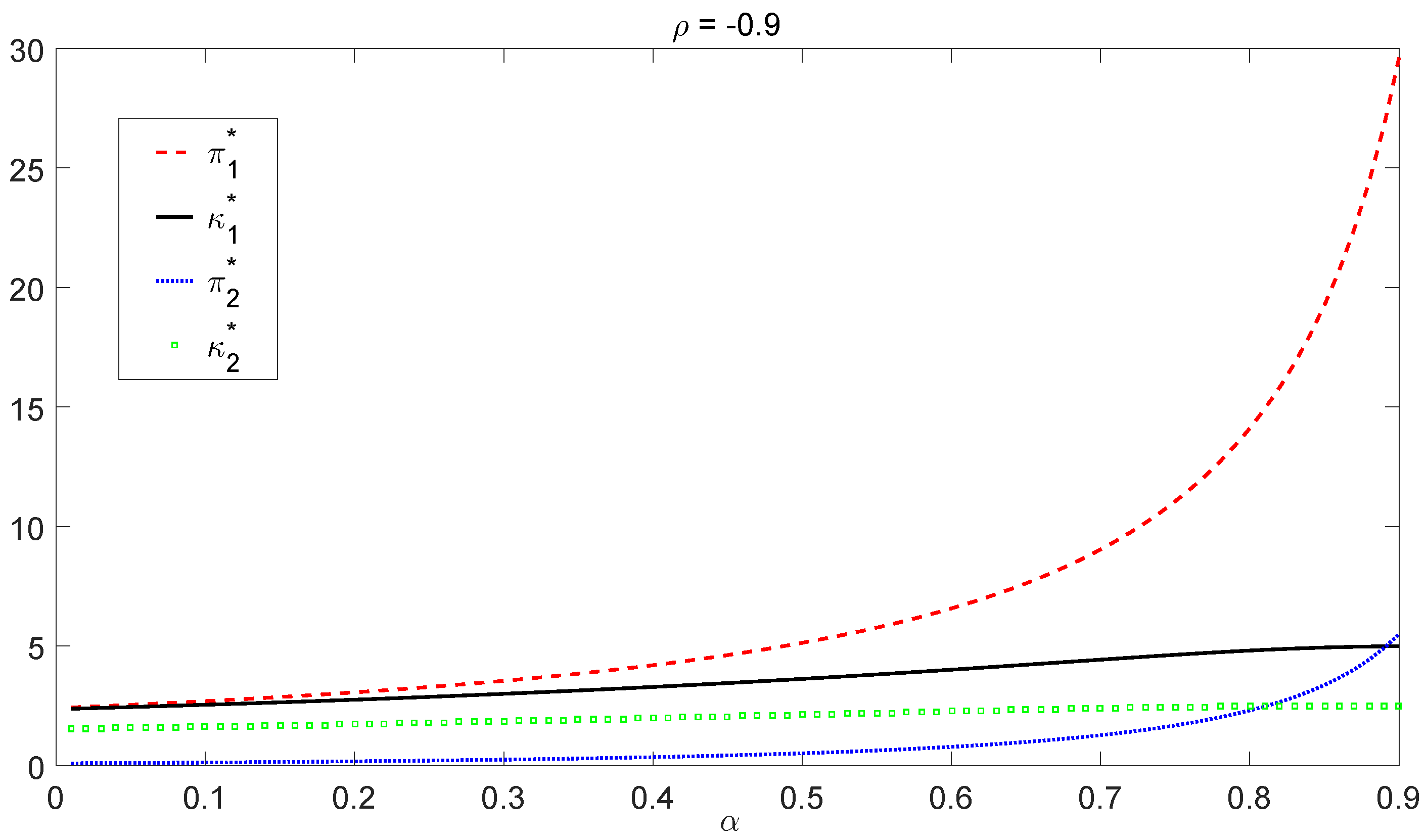
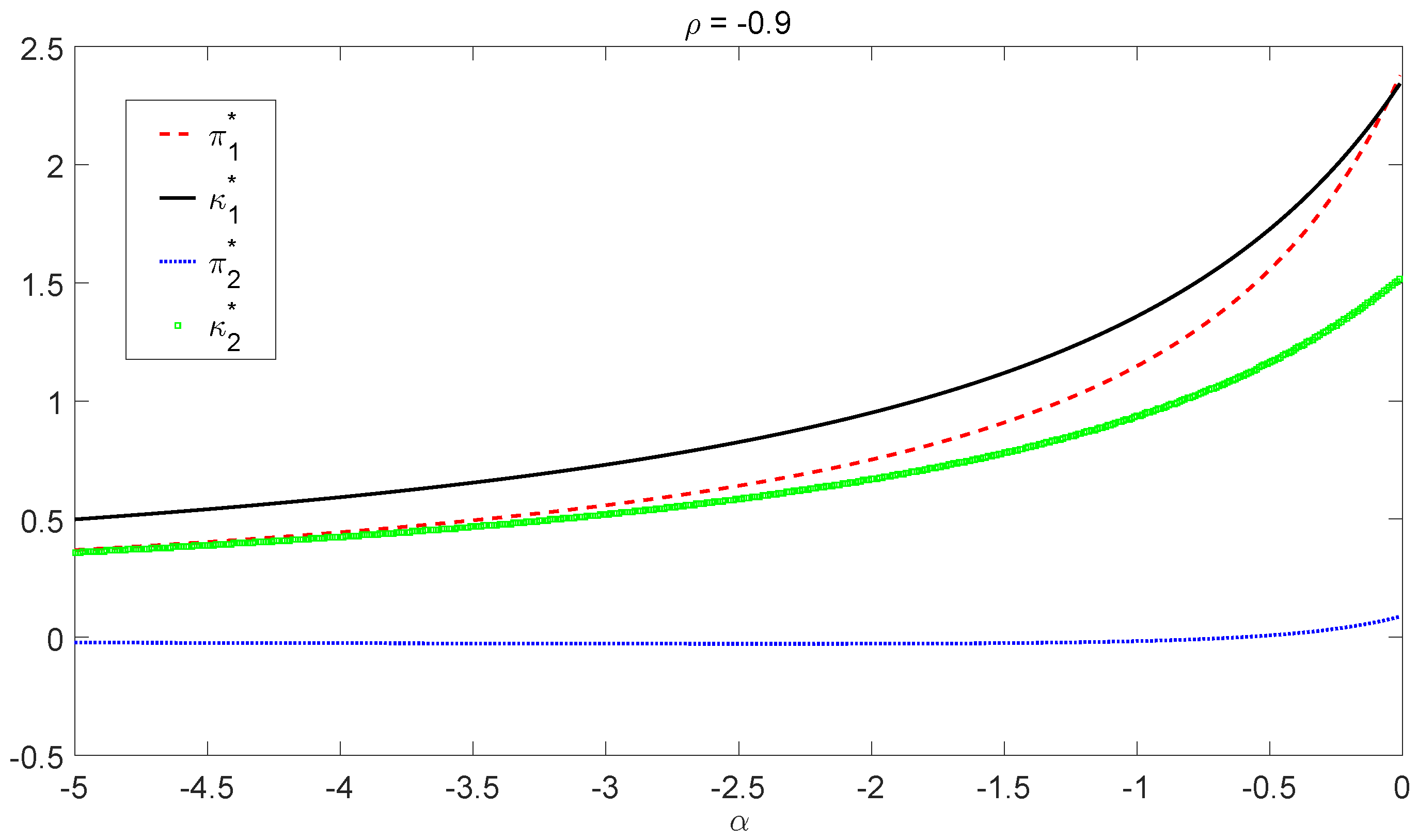
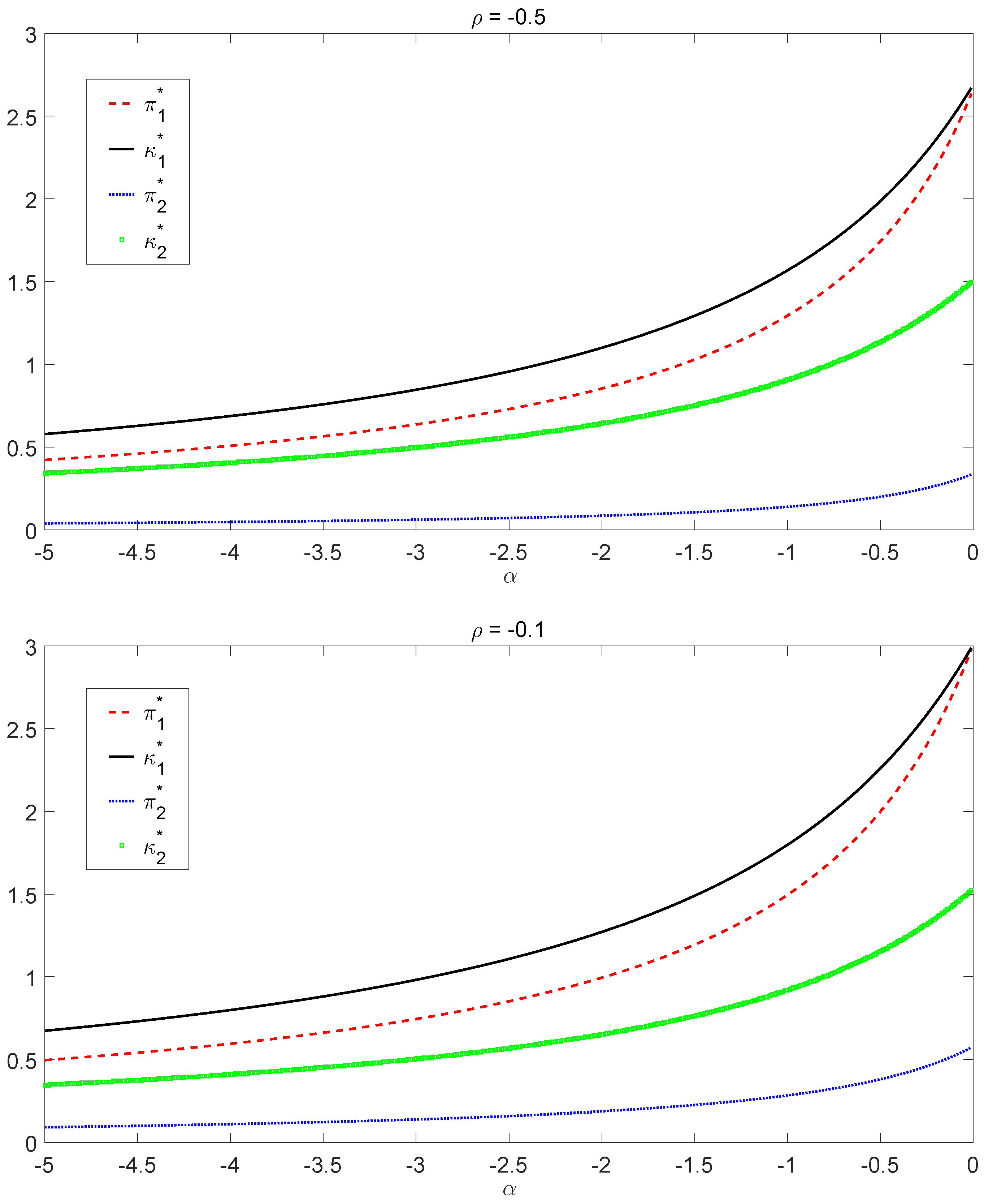
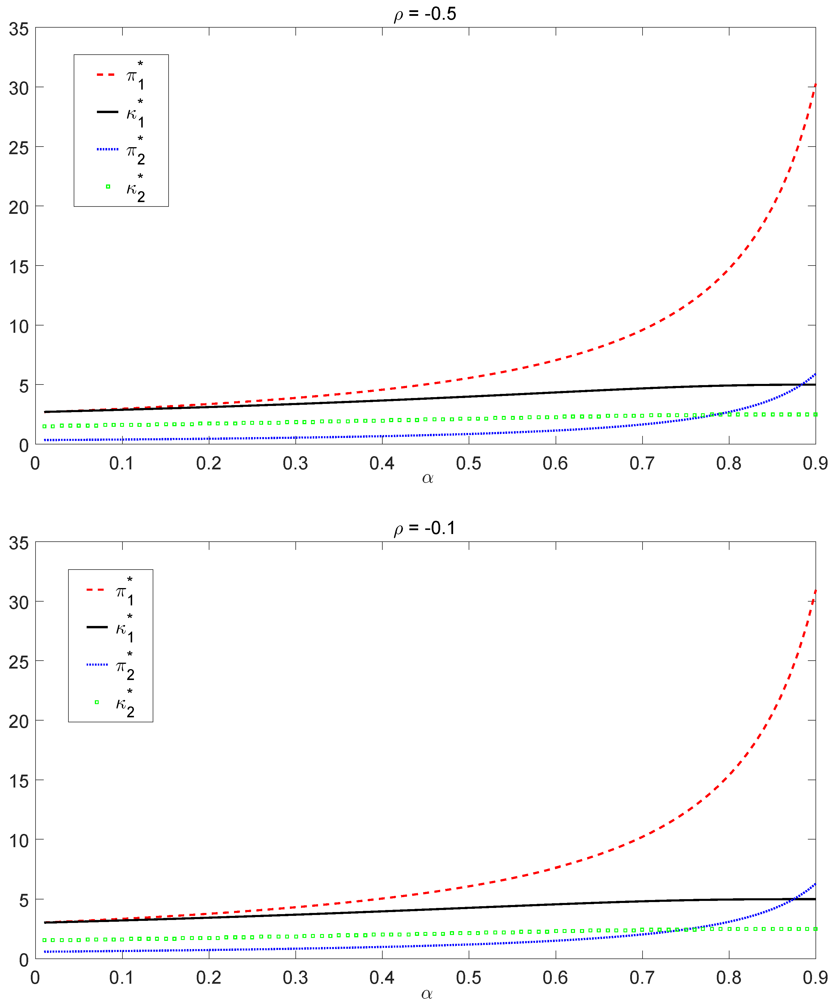
For both high risk-averse ($\alpha <0$) and low risk-averse ($0<\alpha <1$) insurers, we obtain the corresponding optimal policy, given by Equations (23) and (24), through Theorem 3. We plot the optimal policy $u^{*}=({\pi }^{*},{\kappa }^{*})$ as a function of α under three different values of the correlation coefficient ρ. The case $-5<\alpha <0$ is graphed in Figure 1 while the case $0<\alpha <0.9$ is presented in Figure 2. By Equation (18), the optimal investment ${\pi }^{*}$ will explode as α approaches one, so we choose the interval of α to be $(0,0.9)$ instead of $(0,1)$ for low risk-averse insurers.

From the graphs in Figure 1 and Figure 2, we observe that the optimal investment ${\pi }^{*}$ and the optimal liability ratio ${\kappa }^{*}$ are increasing with respect to α in both bull and bear regimes for all chosen ρ. Hence, less risk-averse insurers (that is, insurers with large α) invest proportionally more in the risky asset and choose a higher liability ratio. Figure 1 shows that after α drops below some threshold (e.g., around $-3$ in the bear regime when $\rho =-0.1$), the optimal policy is not sensitive to the change of α, indicating that there exists a “saturation” level for the risk aversion. For high risk-averse insurers (α small enough), risk aversion does not affect the optimal liability ratio ${\kappa }^{*}$, nor the optimal investment ${\pi }^{*}$ that much in both regimes. On the other hand, when α gets close to one, there is a dramatic effect of the risk aversion on the optimal investment ${\pi }^{*}$. In this scenario, the optimal investment ${\pi }^{*}$ will clearly explode due to the factor $\frac{1}{1-\alpha }$ going to infinity. We also notice that borrowing (${\pi }^{*}>1$) is necessary to reach the optimal policies in some cases. Furthermore, the optimal policies obtained in Figure 1 and Figure 2 converge to the one in Table 2 as $\alpha \to 0$ from both sides.

5.2. Analysis on the Impact of the Correlation Coefficient ρ on the Optimal Policy

As pointed out in [21] (Chapter 6), a major mistake that contributed significantly to AIG’s sudden collapse was the negligence of the negative correlation between the risk and the capital returns (equivalently, AIG assumed ${\rho }_i\equiv 0$ instead of ${\rho }_i<0$). Thus, in this subsection, we focus on the impact of the correlation coefficient on the optimal policy.

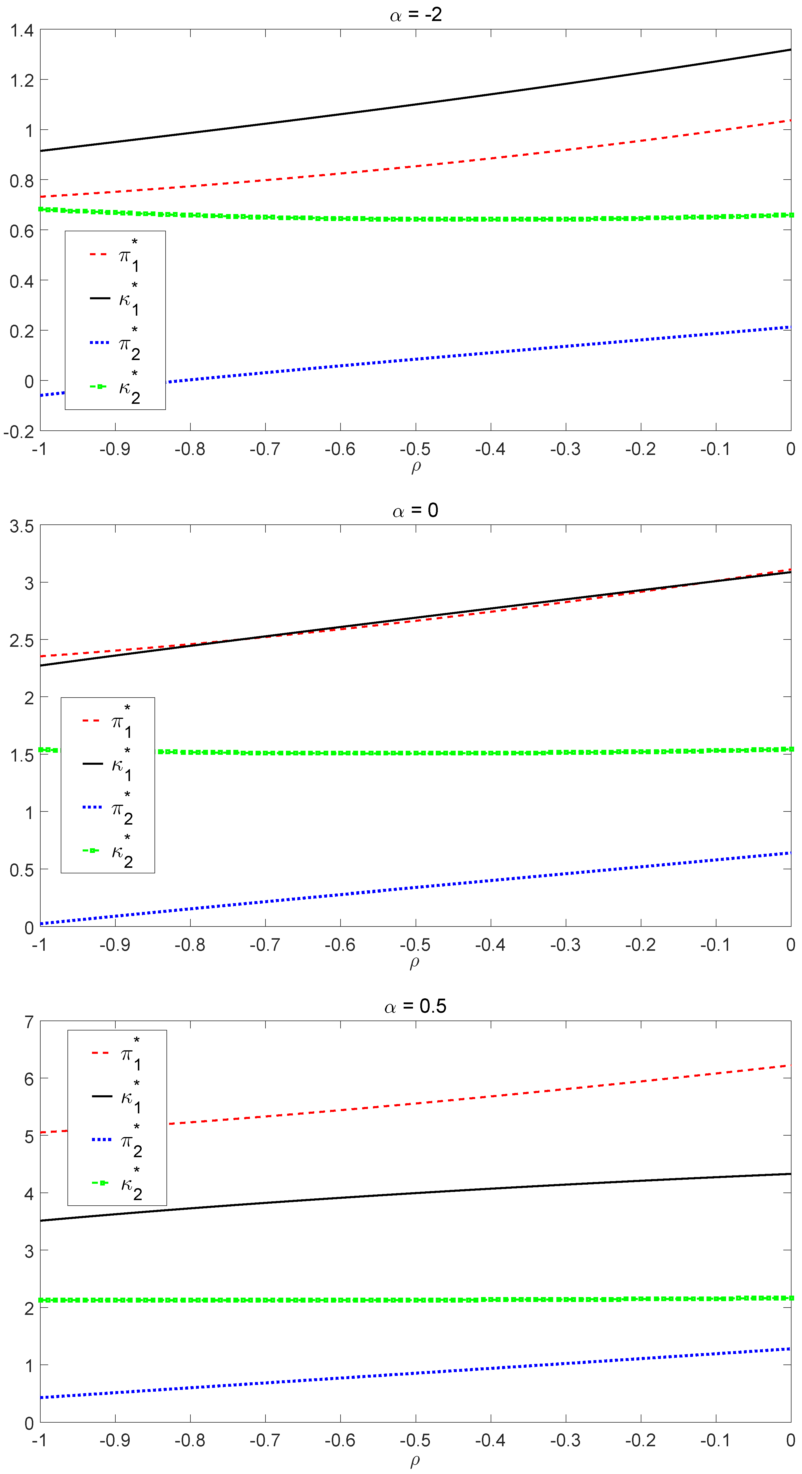
We consider $\alpha =-2,0,$ and $0.5$, representing high risk-averse, moderate risk-averse and low risk-averse insurers, respectively. We first study a simplified case in which the correlation coefficient is the same in both bull and bear regimes, namely $\rho ={\rho }_1={\rho }_2$. Based on the results in Figure 3, we find that the optimal investment strategy ${\pi }^{*}$ is an increasing function of ρ in both regimes and in all cases of α. In addition, since ${\kappa }^{*}$ does not fluctuate significantly with respect to the change of ρ, the increasing magnitude of ${\pi }^{*}$ in ρ is close to linear growth, which is consistent with Equations (10) and (18). However, the impact of ρ on the optimal liability ratio ${\kappa }^{*}$ is more complicated. In the bull market, ${\kappa }^{*}$ increases as the negative correlation strength reduces (that is, ${\kappa }^{*}$ increases as $\left|\rho \right|$ decreases). In the bear market, ${\kappa }^{*}$ is somehow immune to ρ, especially in the case of $\alpha =0.5$. 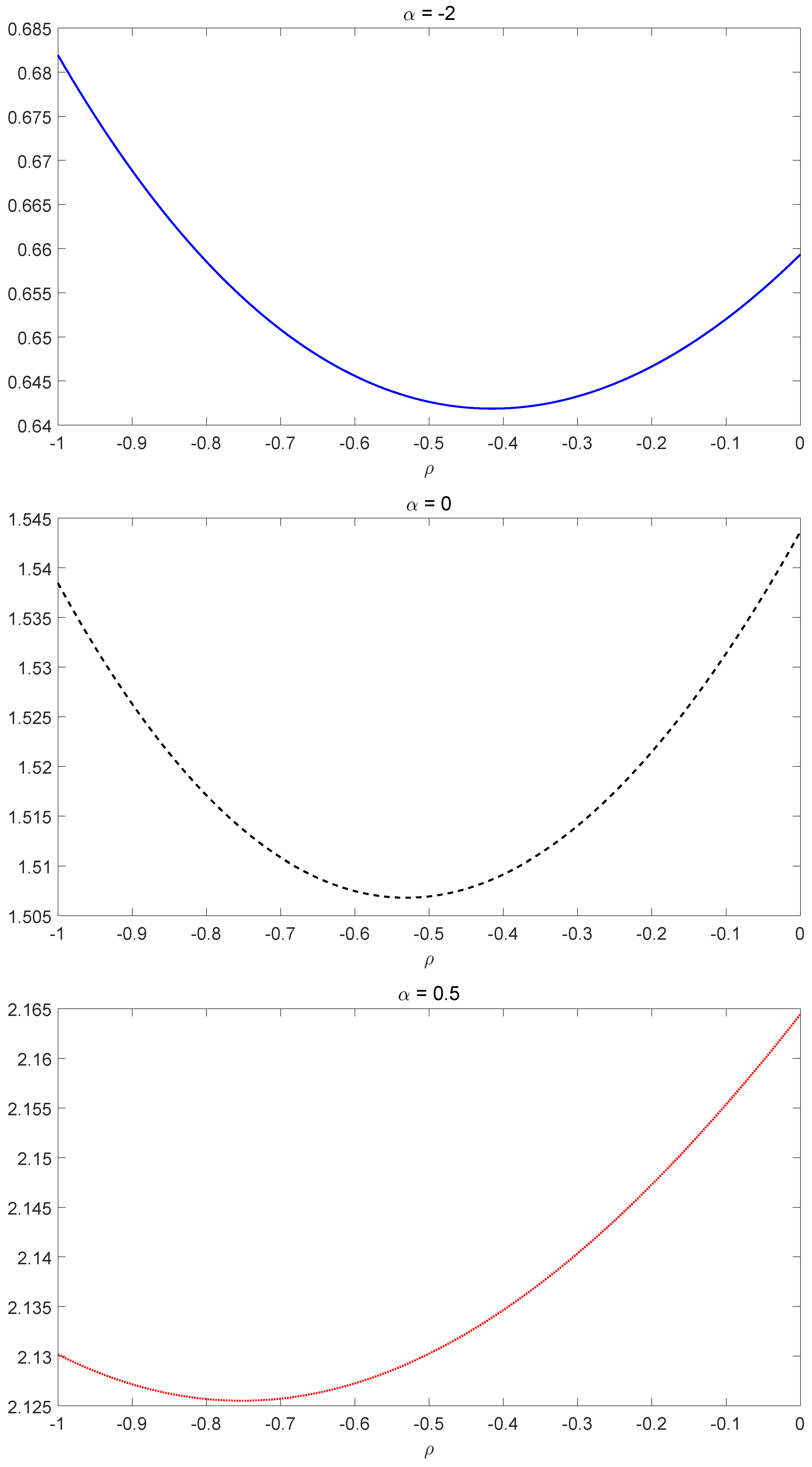To further investigate the relationship between ${\kappa }^{*}$ (${\kappa }_2^{*}$) and ρ in the bear market, we draw the graph of ${\kappa }^{*}$ against ρ separately in Figure 4. We conclude that in the bear market, the optimal liability ratio ${\kappa }_2^{*}$ is a convex function of ρ, where $\rho \in (-1,0)$. This conclusion is consistent with the findings in [22] for the case of only one regime.

Next, we proceed to deal with the more realistic case where $|{\rho }_1|<|{\rho }_2|$ (equivalently, $-1\le {\rho }_2<{\rho }_1<0$), in which the negative correlation between the liabilities and the capital returns is stronger in the bear market. For the basic parameter values (with parameter values given by Table 1), we calculate the optimal policy under the following four cases for ${\rho }_1$ and ${\rho }_2$:

$$\begin{array}{ccc}\hfill \mathrm{Case}1.& & {\rho }_1=-0.7\mathrm{and}{\rho }_2=-0.9\hfill \\ \hfill \mathrm{Case}2.& & {\rho }_1=-0.5\mathrm{and}{\rho }_2=-0.7\hfill \\ \hfill \mathrm{Case}3.& & {\rho }_1=-0.3\mathrm{and}{\rho }_2=-0.5\hfill \\ \hfill \mathrm{Case}4.& & {\rho }_1=-0.1\mathrm{and}{\rho }_2=-0.3.\hfill \end{array}$$

The results are presented in

Table 3. Optimal policy when $|{\rho }_1|<|{\rho }_2|$.

α	Case of ${\mathit{\rho }}_1$ and ${\mathit{\rho }}_2$	${\mathit{\pi }}_1^{*}$	${\mathit{\kappa }}_1^{*}$	${\mathit{\pi }}_2^{*}$	${\mathit{\kappa }}_2^{*}$
$\alpha =-5$	Case 1	0.3932	0.5372	−0.0227	0.3594
	Case 2	0.4221	0.5785	0.0094	0.3474
	Case 3	0.4561	0.6237	0.0383	0.3417
	Case 4	0.4961	0.6737	0.0657	0.3415
$\alpha =-2$	Case 1	0.7983	1.0233	−0.0274	0.6688
	Case 2	0.8537	1.1000	0.0311	0.6508
	Case 3	0.9188	1.1823	0.0848	0.6426
	Case 4	0.9947	1.2714	0.1361	0.6433
$\alpha =0$	Case 1	2.5214	2.5275	0.0905	1.5263
	Case 2	2.6628	2.6900	0.2170	1.5108
	Case 3	2.8261	2.8502	0.3386	1.5069
	Case 4	3.0108	3.0088	0.4583	1.5140
$\alpha =0.2$	Case 1	3.2027	2.9408	0.1760	1.7333
	Case 2	3.3696	3.1157	0.3178	1.7220
	Case 3	3.5606	3.2827	0.4558	1.7211
	Case 4	3.7741	3.4426	0.5924	1.7299
$\alpha =0.5$	Case 1	5.3301	3.8234	0.5142	2.1272
	Case 2	5.5565	3.9941	0.6848	2.1257
	Case 3	5.8080	4.1423	0.8539	2.1303
	Case 4	6.0799	4.2711	1.0232	2.1404

, which are consistent with the findings when ${\rho }_1={\rho }_2$ above.2 Namely, we still observe that the optimal investment in both regimes (${\pi }_1^{*}$ and ${\pi }_2^{*}$) and the optimal liability ratio in the bull regime (${\kappa }_1^{*}$) are increasing with respect to ${\rho }_i$, $i=1,2$, while the optimal liability ratio in the bear regime (${\kappa }_2^{*}$) is a convex function of ${\rho }_i$, $i=1,2$. We also notice that in some cases, ${\pi }_2^{*}$ is negative, which means the optimal investment involves short-selling the risky asset.

It is surprising to observe that in the case $\alpha =-5$, ${\kappa }^{*}$ is not only a convex function, but also increases as the economy goes from Case 4–Case 1. To understand this situation, we consider only two regimes and rewrite Equation (18) in the form:

$${\pi }^{*}-{\mathbb{I}}_i{\kappa }^{*}={\mathbb{J}}_i,$$

where:

$${\mathbb{I}}_i=\frac{b_i{\rho }_i}{{\sigma }_i}<0\mathrm{and}{\mathbb{J}}_i=\frac{1}{(1-\alpha )}\frac{{\mu }_i-r_i}{{\sigma }_i^2}>0.$$

We recall that we are assuming $\frac{{\mu }_1-r_1}{{\sigma }_1^2}>\frac{{\mu }_2-r_2}{{\sigma }_2^2}$, as supported by [31]. Thus, when the economy is good, both ${\pi }^{*}$ and ${\kappa }^{*}$ take large positive values. That is not surprising and agrees with the above equation. When the economy is bad, ${\mathbb{J}}_i$ approaches zero, especially when the investor is very risk averse. In addition, ${\rho }_i$ approaches $-1$. In a case of severe recession, ${\pi }^{*}$ would take even negative values. To compensate for that, the above equation says that ${\kappa }^{*}$ should take large positive values.

5.3. Analysis of the Impact of the Regimes on the Optimal Policy

The numerical results obtained in Section 5.1 and Section 5.2 allow us to reach some conclusions on the impact of the market regimes on the optimal policy.

In all of the above studies, the optimal policy depends on the market regime. Furthermore, we always have:

$${\pi }_1^{*}>{\pi }_2^{*}\mathrm{and}{\kappa }_1^{*}>{\kappa }_2^{*}.$$

This result shows that all insurers, regardless of risk aversion, should invest a greater proportion in the risky asset and choose a higher liability ratio when the economy is in the bull regime.

6. Conclusions

The 2007–2009 financial crisis brought new challenges on risk management to all market participants. For instance, AIG did not follow proper risk management strategies and, as a consequence, almost went bankrupt in 2008. There were two major contributors to AIG’s sudden collapse. First, AIG did not pay full attention to the business cycles (regime switching) in the U.S. housing market, which directly caused a significant underestimation of the risk of CDS policies. Second, AIG ignored the negative correlation between its liabilities and the capital gains in the financial market.

Taking the lessons from the AIG case, we set up a regime switching model from an insurer’s perspective. In the model, we assume that not only the financial market, but also the insurer’s risk process depend on the regime of the economy. An insurer makes investment decisions in a financial market, which consists of a riskless asset and K risky assets, and faces an external risk that is negatively correlated with the capital returns of the risky assets. The insurer wants to maximize her/his expected utility of terminal wealth by selecting simultaneously the optimal investment proportions in the risky assets and the optimal liability ratio. We obtain explicitly optimal investment and liability ratio policies when the insurer’s utility is given by the logarithmic and power utility functions.

Through an economic analysis, we find that the optimal policy depends strongly on both the business cycles (market regimes) and the negative correlation between the liabilities and the capital returns. To be more specific, all insurers should invest a greater proportion in the risky assets and select a higher liability ratio when the market is in a bull regime. The optimal investment proportions in the risky assets are increasing with respect to ρ (correlation coefficient) in both bull and bear regimes. The relationship between the optimal liability ratio and ρ is more complicated: there is an increasing relationship in the bull regime and a convex relationship in the bear regime. Furthermore, we find that the optimal investment proportions and the optimal liability ratios are increasing functions of α (risk aversion parameter) in both market regimes. That means a less risk-averse insurer will invest a greater proportion in the risky assets and select a higher liability ratio, no matter what regime the market is in.