
Actuarial Geometry


St. John’s University, Peter J. Tobin College of Business, 101 Astor Place, New York, NY 10003, USA
Risks 2017, 5(2), 31; https://doi.org/10.3390/risks5020031
Submission received: 12 April 2017
/
Revised: 16 May 2017
/
Accepted: 2 June 2017
/
Published: 16 June 2017
(This article belongs to the Special Issue A Celebration of the Ties That Bind Us: Connections between Actuarial Science and Mathematical Finance)
Abstract
:The literature on capital allocation is biased towards an asset modeling framework rather than an actuarial framework. The asset modeling framework leads to the proliferation of inappropriate assumptions about the effect of insurance line of business growth on aggregate loss distributions. This paper explains why an actuarial analog of the asset volume/return model should be based on a Lévy process. It discusses the impact of different loss models on marginal capital allocations. It shows that Lévy process-based models provide a better fit to the US statutory accounting data, and identifies how parameter risk scales with volume and increases with time. Finally, it shows the data suggest a surprising result regarding the form of insurance parameter risk.
1. Introduction
Geometry is the study of shape and change in shape. Actuarial Geometry1 studies the shape and evolution of shape of actuarial variables, in particular the distribution of aggregate losses, as portfolio volume and composition changes. It also studies the shape and evolution paths of variables in the space of all risks. Actuarial variables are curved across both a volumetric dimension as well as a temporal dimension. Volume here refers to expected losses per year, x, and temporal to the duration, t, for which a given volume of insurance is written. Total expected losses are —just as distance = speed × time. Asset variables are determined by a curved temporal return distribution but are flat in the volumetric (position size) dimension. Risk, and hence economic quantities like capital, are intimately connected to the shape of the distribution of losses, and so actuarial geometry is inextricably linked to capital determination and allocation.
Actuarial geometry is especially important today because risk and probability theory, finance, and actuarial science are converging after prolonged development along separate tracks. There is now general agreement that idiosyncratic insurance risk matters for pricing, and as a result we need to appropriately understand, model, and reflect the volumetric and temporal diversification of insurance risk. These are the central topics of the paper.
The paper makes two research contributions both linked to the use of Lévy processes in actuarial science. The first contribution is theoretical. It is to explain precisely how insurance losses diversify as volume increases and to compute the impact of this diversification compared to an asset portfolio model where risk is independent of position size. In particular we show that even when insurance losses and an asset portfolio have the same distribution of outcomes for a particular volume, the agreement is that of two lines crossing at an angle. It is not a first order tangency and so any risk allocation involving derivatives—which almost all do—will produce different results. The picture we make precise is shown in Figure 1. In the figure k is the distribution of values of an asset portfolio with initial value x, modeled as for a fixed return variable X. The map m represents aggregate losses from an insurance portfolio with expected losses x. Even though the tangent vector, , to the embedding m at is not the same as the tangent vector . We have drawn m as a straight line because it will naturally capture the idea of “growth in the direction X”. The full rationale behind Figure 1 is described in Section 6.
The second contribution is empirical. It uses US statutory accounting data to determine a Lévy process based model for insurance losses by line of business that reflects their observed volumetric and temporal properties. The analysis compares four potential models and determines that only one is consistent with the data. The analysis produces specific line of business measures of non-diversifiable parameter risk that vary substantially but that have been consistent over time. It also provides an explicit form for the distribution of parameter risk, even though parameter risk cannot be directly observed. Most papers on risk measures take the actual distribution of losses as given. And much work done by companies to quantify risk is regarded as proprietary and is not published. The explicit quantification we provide should therefore be useful as a benchmark for both academics and practicing actuaries.
The remainder of the paper is organized as follows.
Section 2 describes the how actuaries and academics came to agree, over the last century, that idiosyncratic insurance risk matters for pricing. This agreement provides an important motivation for our theoretical and empirical work.
Section 3 defines a risk measure and explains how the allocation problem naturally leads to the derivative and gradient of a risk measure.
Section 4 presents two motivating examples that it is instructive to keep in mind through the rest of the paper, and which also illustrate Figure 1.
Section 5 defines Lévy processes and gives some basic examples. It then defines four Lévy process-based loss models that will be used as candidate models for aggregate losses, as well as an alternative asset-based model, and it establishes some of their basic properties.
Section 6 is the technical heart of the paper. It investigates the definition of derivative for a real function and considers how it could be defined on more general spaces, such as the space of random variables. It explains how Lévy processes can be used to define “direction” and how the infinitesimal generator of a Lévy process relates to derivatives. This allows us to pin-point the difference between the derivatives of an insurance process and of an asset process.
Section 7 is contains all the empirical results in the paper. It shows how we can effectively quantify parameter risk, even though it cannot be observed directly. It then determines the amount and shape of parameter risk across many lines of business. Finally, it addresses the differences between temporal and volumetric growth.
The paper covers topics from a variety of viewpoints befitting an article in this special edition celebrating the connections between actuarial science and mathematical finance. As a result it is quite long. Readers more interested in the theoretical findings can focus on Section 4, Section 5.1, Section 5.2 and Section 6. Readers more interested in the empirical analysis can focus on Section 5.1, Section 5.2 and Section 7.
2. Why Idiosyncratic Insurance Risk Matters
In its early years property-casualty actuarial science in the US largely ignored risk theory in rate making because of the dominance of bureau-based rates. Property rates were made to include a 5% profit provision and a 1% contingency provision; they were priced to a 94% combined ratio Magrath (1958). Lange (1966) describes a 5% provision for underwriting and contingencies as “constant for all liability insurance lines in most states”. Kallop (1975) states that a 2.5% profit and contingency allowance for workers’ compensation has been in use for at least 25 years and that it “contemplates additional profits from other sources to realize an adequate rate level”. The higher load for property lines was justified by the possibility of catastrophic losses—meaning large conflagration losses rather than today’s meaning of hurricane or earthquake related, severity driven events.
Regulators and actuaries started to consider improvements to these long-standing conventions in the late 1960s. Bailey (1967) introduced actuaries to the idea of including investment income in profit. Ferrari (1968) was the first actuarial paper to include investment income and to consider return on investor equity as well as margin on premium. During the following dozen years actuaries developed the techniques needed to include investment income in ratemaking. At the same time, finance began to consider how to determine a fair rate of return on insurance capital. The theoretical results they derived, summarized as of 1987 in Cummins and Harrington (1987), focused on the use of discounted cash flow models using CAPM-derived discount rates for each cash flow, including taxes. Since CAPM only prices systematic risk, a side-effect of the financial work was to de-emphasize details of the distribution of ultimate losses in setting the profit provision.
At the same time option and contingent claim theoretic methods, (Doherty and Garven 1986; Cummins 1988), were developed as another approach to determining fair premiums. Interest in option theoretic models was motivated in part by the difficulty of computing appropriate s. These papers applied powerful results from option pricing theory using a geometric Brownian motion to model losses, possibly with a jump component. Cummins and Phillips (2000) and D’Arcy and Doherty (1988) contain a summary of the CAPM and contingent claims approaches from a finance perspective and D’Arcy and Dyer (1997) contains a more actuarial view.
The CAPM-based theories failed to explain the observed fact that insurance companies charged for specific risk. A series of papers, beginning in the early 1990s, developed a theoretical explanation of this based around agency, taxation and regulatory costs of capital, certainty in capital budgeting, costly external capital for opaque intermediaries, contracting under asymmetric information, and adverse selection, see Cummins (2000); Froot and O’Connell (2008); Froot and Stein (1998); Froot et al. (1993); Froot (2007); Merton and Perold (2001); Perold (2001); Zanjani (2002).
At the same time banking regulation led to the development of robust risk measures and an axiomatic theory of risk measures, including the idea of a coherent measure of risk Artzner et al. (1999). Risk measures are sensitive to the particulars of idiosyncratic firm risk, unlike the CAPM-based pricing methods which are only concerned with systemic risks.
The next step was to develop a theory of product pricing for a multiline insurance company within the context of costly firm-specific risk and robust risk measures. This proceeded down two paths. Phillips et al. (1998) considered pricing in a multiline insurance company from a complete-market option theoretic perspective, modeling losses with a geometric Brownian motion and without allocating capital. They were concerned with the effect of firm-wide insolvency risk on individual policy pricing.
The second path, based around explicit allocation of capital, was started by Myers and Read (2001). They also worked in a complete market setting and used expected default value as a risk measure, determined surplus allocations by line, and presented a gradient vector, Euler theorem based allocation assuming volumetrically homogeneous losses—but making no other distributional assumptions. This thread was continued by Tasche (1999), Denault (2001) and Fischer (2003). Sherris (2006) takes the view that, in a complete market setting, only the default put has a canonical allocation and that there is no natural allocation of the remaining capital—a view echoed by Gründl and Schmeiser (2007). Kalkbrener (2005) and Delbaen (2000a) used directional derivatives to clarify the relationship between risk measures and allocations.
Concepts from banking regulation, including an own risk solvency assessment, have been adopted by insurance regulators and have led to increased academic interest in technical aspects of risk measurement, capital allocation and risk based pricing. A focus on catastrophe reinsurance pricing following the US hurricanes of 2004 and 2005 and the development of a robust capital market alternative to traditional reinsurance has also motivated research. As a result there is now a very rich literature around this nexus, including the following.
- Technical and axiomatic characterization of risk measures: (Dhaene et al. 2003; Furman and Zitikis 2008; Laeven and Stadje 2013).
- Capital allocation and its relationship with risk measurement: (Dhaene et al. 2003; Venter et al. 2006; Bodoff 2009; Buch and Dorfleitner 2008; Dhaene et al. 2012; Erel et al. 2015; Furman and Zitikis 2008; Powers 2007; Tsanakas 2009).
- The connection between purpose and method in capital allocation: (Dhaene et al. 2008; Zanjani 2010; Bauer and Zanjani 2013b; Goovaerts et al. 2010).
- Questioning the need for capital allocation in pricing: Gründl and Schmeiser 2007.
With the confluence of these different theoretical threads, and, in particular, in light of the importance of firm-specific risk to insurance pricing, the missing link—and the link considered in this paper—is a careful examination of the underlying actuarial loss distribution assumptions. Unlike traditional static distribution-based pricing models, such as standard deviation and utility, modern marginal and differential methods require explicit volumetric and temporal components. The volumetric and temporal geometry are key to the differential calculations required to perform risk and capital allocations. All of the models used in the papers cited are, implicitly or explicitly, volumetrically homogeneous and geometrically flat in one dimension. For example, in a geometric Brownian motion model losses at time t are of the form where is a Brownian motion. Changing volume, , simply scales the whole distribution and does not affect the shape of the random component. The jump-diffusion model in Cummins (1988) is of the same form. There are essentially no other explicit loss models in the papers cited. Mildenhall (2004) and Meyers (2005b) show volumetric homogeneity is not an appropriate assumption. This paper provides further evidence and uses insurance regulatory data to explore more appropriate models.
3. Risk Measures, Risk Allocation and the Ubiquitous Gradient
3.1. Definition and Examples of Risk Measures
A risk measure, , is a real valued function defined on a space of risks . Here is the sample space, is a sigma-algebra of subsets of , and is a probability measure on . The space consists of all real valued random variables, that is, measurable functions , defined up to equivalence (identify random variables which differ on a set of measure zero). As Delbaen (2000b) points out there are only two spaces which are invariant under equivalent measures, and , the space of all essentially bounded random variables. Since it is desirable to work with a space invariant under change of equivalent measure, but not to be restricted to bounded variables, we work with . Kalkbrener (2005) works on . Risk measures are a large and important topic, but their details are not central this paper. For more details see Föllmer and Schied (2011) and Dhaene et al. (2006).
Given a risk , is the amount of capital required to support the risk. Examples of risk measures include value at risk at a percentile (the inverse of the distribution of X, defined as ), tail value at risk (the average of the worst outcomes), and standard deviation .
3.2. Allocation and the Gradient
At the firm level, total risk X can be broken down into a sum of parts corresponding to different lines of business. Since it is costly for insurers to hold capital Froot and O’Connell (2008) it is natural to ask for an attribution of total capital to each line . One way to do this is to consider the effect of a marginal change in the volume of line i on total capital. For example, if the marginal profit from line i divided by the marginal change in total capital resulting from a small change in volume in line i exceeds the average profit margin of the firm then it makes sense to expand line i. This is a standard economic optimization that has been discussed in the insurance context by many authors including Tasche (1999), Myers and Read (2001), Denault (2001), Meyers (2005b) and Fischer (2003).
The need to understand marginal capital leads us to consider
which, in a sense to be made precise, represents the change in as a result of a change in the volume of line i, or more generally the gradient vector of representing the change across all lines. Much of this paper is an examination of exactly what this equation means.
Tasche (1999) shows that the gradient vector of the risk measure is the only vector suitable for performance measurement, in the sense that it gives the correct signals to grow or shrink a line of business based on its marginal profitability and marginal capital consumption. Tasche’s framework is unequivocally financial. He considers a set of basis asset return variables , and then determines a portfolio as a vector of asset position sizes . The portfolio value distribution corresponding to x is simply
A risk measure on induces a function , . Rather than being defined on a space of random variables, the induced is defined on (a subset of) Euclidean space using the correspondence between x and a portfolio. In this context is simply the usual limit
Equation (3) is a powerful mathematical notation and it contains two implicit assumptions. First, the fact that we can write requires that we can add in the domain. If were defined on a more general space this may not possible—or it may involve the convolution of measures rather than addition of real numbers. Second, and more importantly, adding to x in the ith coordinate unambiguously corresponds to an increase “in the direction” of the ith asset. This follows directly from the definition in Equation (2) and is unquestionably correct in a financial context.
Numerous papers work in an asset/volume model framework, either because they are working with assets or as a simplification of the real insurance world, for example (Myers and Read 2001; Panjer 2001; Erel et al. 2015; Fischer 2003). The resulting risk process homogeneity is essential to all Euler-based “adds-up” results: in fact the two are equivalent for homogeneous risk measures (Mildenhall 2004; Tasche 2004). However, it is important to realize that risk can be measured appropriately with a homogeneous risk measure, that is one satisfying , even if the risk process itself is not homogeneous, that is . The compound Poisson process and Brownian motion are examples of non-homogeneous processes.
In order to consider alternatives to the asset/return framework, we now discuss the meaning of the differential and examine other possible definitions. The differential represents the best linear approximation to a function at a particular point in a given direction. Thus the differential to a function f, at a point x in its domain, can be regarded as a linear map which takes a direction, i.e., a tangent vector at x, to a direction at . Under appropriate assumptions, the differential of f at in direction , , is defined by the property
see Abraham et al. (1988) or Borwein and Vanderwerff (2010). The vector is allowed to tend to from any direction, and Equation (4) must hold for all of them. This is called Fréchet differentiability. There are several weaker forms of differentiability defined by restricting the convergence of to . These include the Gâteaux differential, where with , , the directional differential, where with , , and the Dini differential, where for , , and . The function if and is not differentiable at , in fact it is not even continuous, but all directional derivatives exist at , and f is Gâteaux differentiable. The Gâteaux differential need not be linear in its direction argument.
Kalkbrener (2005) applied Gâteaux differentiability to capital allocation. The Gâteaux derivative can be computed without choosing a set of basis asset return-like variables, that is without setting up a map from , provided it is possible to add in the domain. This is the case for because we can add random variables. The Gâteaux derivative of at in the direction is defined as
Kalkbrener shows that if the risk measure satisfies certain axioms then it can be associated with a unique capital allocation. He shows that the allocation is covariance-based if risk is measured using standard deviation and a conditional measure approach when risk is measured by expected shortfall—so his method is very natural.
We have shown that notions of differentiability are central to capital allocation. The next section will present two archetypal examples and that show the asset/return and insurance notions of growth do not agree, setting up the need for a better understanding of “direction” for actuarial random variables. We will see that Lévy processes provide that understanding.
4. Two Motivating Examples
This section presents two examples illustrating the difference between an asset/return model and a realistic insurance growth model.
Let be a Poisson random variable with mean u. Consider two functions, and . The function k defines a random variable with mean u and standard deviation u. The function m also defines a random variable with has mean u, but it has standard deviation . The variable k defines a homogeneous family, that is , and correctly models the returns from a portfolio of size u in an asset with an (unlikely) Poisson(1) asset return distribution. The variable m is more realistic for a growing portfolio of insurance risks with expected annual claim count u.
If we measure risk using the standard deviation risk measure , this example shows that although have the same distribution the marginal risk for k is whereas the marginal risk for m is . For m risk decreases as volume increases owing to portfolio effects whereas for k there is no diversification.
Next we present a more realistic example, due to Meyers (2005a), where Kalkbrener’s “axiomatic” allocation produces a different result than a marginal business written approach that is based on a more actuarial set of assumptions. Meyers calls his approach “economic” since it is motivated by the marginal increase in business philosophy discussed in Section 3.2. This example has also been re-visited recently by Boonen et al. (2017).
In order to keep the notation as simple as possible the example works with independent lines of business and allocates capital to line 1 . The risk measure is standard deviation for . Losses are modeled with a mixed compound Poisson variable
where is a -mixed Poisson, so the conditional distribution is Poisson with mean and the mixing distribution has mean 1 and variance . Meyers calls the contagion. The mixing distributions are often taken to be gamma variables, in which case each has a negative binomial distribution. The , are independent, identically distributed severity random variables. For simplicity, assume that , so that . Since the model only considers volumetric diversification and not temporal diversification.
We can compute as follows:
where . Note that for any constant k.
Kalkbrener’s axiomatic capital is computed using the Gâteaux directional derivative. Let and note that . Then, by definition and the independence of and , the Gâteaux derivative of at in the direction is
This whole calculation has been performed without picking an asset return basis, but it can be replicated if we do. Specifically, use the as a basis and define a linear map of -vector spaces , by . Let be the composition of k and ,
Then
agreeing with Equation (7). It is important to remember that for .
Given the definition of , we can also define an embedding , by . The map m satisfies but it is not a linear map of real vector spaces because . In fact, the image of m will generally be an infinite dimensional real vector subspace of . The lack of homogeneity is precisely what produces a diversification effect. As explained in Section 3.2, an economic view of capital requires an allocation proportional to the gradient vector at the margin. Thus capital is proportional to where is the composition of m and ,
Since a real function, we can compute its partial derivative using standard calculus:
5. Lévy process Models of Insurance Losses
We define Lévy processes and discuss some of their important properties. We then introduce four models of insurance risk which we will analyze in the rest of the paper.
5.1. Definition and Basic Properties of Lévy processes
Lévy processes are fundamental to actuarial science, but they are rarely discussed explicitly in basic actuarial text books. For example, there is no explicit mention of Lévy processes in Bowers et al. (1986); Beard et al. (1969); Daykin et al. (1994); Klugman et al. (1998); Panjer and Willmot (1992). However, the fundamental building block of all Lévy processes, the compound Poisson process, is well known to actuaries. It is instructive to learn about Lévy processes in an abstract manner as they provide a very rich source of examples for modeling actuarial processes. There are many good textbooks covering the topics described here, including Feller (1971) volume 2, Breiman (1992), Stroock (1993), Bertoin (1996), Sato (1999), and Barndorff-Nielsen et al. (2001), and Applebaum (2004).
Definition 1.
A Lévy process is a stochastic process defined on a probability space satisfying
- LP1.
- almost surely;
- LP2.
- X has independent increments, so for the variables are independent;
- LP3.
- X has stationary increments, so has the same distribution as ; and
- LP4.
- X is stochastically continuous, so for all and
Based on the definition it is clear that the sum of two Lévy processes is a Lévy process. Lévy processes are in one-to-one correspondence with the set of infinitely divisible distributions, where X is infinitely divisible if, for all integers , there exist independent, identically distributed random variables so that X has the same distribution as . If is a Lévy process then is infinitely divisible since , and conversely if X is infinitely divisible there is a Lévy process with . In an idealized world, insurance losses should follow an infinitely divisible distribution because annual losses are the sum of monthly, weekly, daily, or hourly losses. Bühlmann Bühlmann (1970) discusses infinitely divisible distributions and their relationship with compound Poisson processes. The Poisson, normal, lognormal, gamma, Pareto, and Student t distributions are infinitely divisible; the uniform is not infinitely divisible, nor is any distribution with finite support, nor any whose moment generating function takes the value zero, see Sato (1999).
Example 1 (Trivial process).
for a constant k is a trivial Lévy process.
Example 2 (Poisson process).
The Poisson process with intensity λ has
for is a Lévy process.
Example 3 (Compound Poisson process).
The compound Poisson process with severity component Z is defined as
where is a Poisson process with intensity λ. The compound Poisson processes is the fundamental building block of Lévy processes in the sense that any infinitely divisible distribution is the limit distribution of a sequence of compound Poisson distributions, see Sato (1999) Corollary 8.8
Example 4 (Brownian motion).
Brownian motion is an example of a continuous Lévy process.
Example 5 (Operational time).
Lundberg introduced the notion of operational time transforms in order to maintain stationary increments for compound Poisson distributions. Operational time is a risk-clock which runs faster or slower in order to keep claim frequency constant. It allows seasonal and daily effects (rush hours, night-time lulls, etc.) without losing stationary increments. Operational time is an increasing function chosen so that becomes a Lévy process.
Example 6 (Subordination).
Let be a Lévy process and let be a subordinator, that is, a Lévy process with non-decreasing paths. Then is also a Lévy process. This process is called subordination and Y is subordinate to X. Z is called the directing process. Z is a random operational time.
The characteristic function of a random variable X with distribution is defined as for . The characteristic function of a Poisson variable with mean is . The characteristic function of a compound Poisson process is
where is the distribution of severity . The characteristic equation of a normal random variable is
We now quote an important result in the theory of Lévy processes that allows us to identify an infinitely divisible distribution, and hence a Lévy process, with a measure on , and two constants and .
Theorem 1 (Lévy-Khintchine).
If the probability distribution μ is infinitely divisible then its characteristic function has the form
where ν is a measure on satisfying and , and . The representation by is unique. Conversely given any such triple there exists a corresponding infinitely divisible distribution.
See Breiman (1992) or Sato (1999) a proof. In Equation (18), is the standard deviation of a Brownian motion component, and is called the Lévy measure. The indicator function is present for technical convergence reasons and is only needed when there are a very large number of very small jumps. If it can be omitted and the resulting can be interpreted as a drift. In the general case does not have a clear meaning as it is impossible to separate drift from small jumps. The indicator can therefore also be omitted if , and in that case the inner integral can be written as
where is a distribution. Comparing with Equation (17) shows this term corresponds to a compound Poisson process.
The triples in the Lévy-Khintchine formula are called Lévy triples. The Lévy process corresponding to the Lévy triple has triple .
The Lévy-Khintchine formula helps characterize all subordinators. A subordinator must have a Lévy triple with no diffusion component (because Brownian motions take positive and negative values) and the Lévy measure must satisfy , i.e., have no negative jumps, and . In particular, there are no non-trivial continuous increasing Lévy processes.
The insurance analog of an asset return portfolio basis becomes a set of Lévy processes representing losses in each line of business and “line” becomes synonymous with the Lévy measure that describes the frequency and severity of the jumps, i.e., of the losses. Unless the Lévy process has an infinite number of small jumps the Lévy measure can be separated into a frequency component and a severity component. Patrik et al. (1999) describes modeling with Lévy measures, which the authors call a loss frequency curve.
5.2. Four Temporal and Volumetric Insurance Loss Models
We now define four models describing how the total insured loss random variable evolves volumetrically and temporally. Let the random variable denote aggregate losses from a line with expected annual loss x that is insured for a time period t years. Thus is the distribution of annual losses. The central question of the paper is to describe appropriate models for as x and t vary. A Lévy process provides the appropriate basis for modeling . We consider four alternative insurance models.
- IM1.
- . This model assumes there is no difference between insuring given insureds for a longer period of time and insuring more insureds for a shorter period.
- IM2.
- , for a subordinator with . Z is an increasing Lévy process which measures random operational time, rather than calendar time. It allows for systematic time-varying contagion effects, such as weather patterns, inflation and level of economic activity, affecting all insureds. Z could be a deterministic drift or it could combine a deterministic drift with a stochastic component.
- IM3.
- , where C is a mean 1 random variable capturing heterogeneity and non-diversifiable parameter risk across an insured population of size x. C could reflect different underwriting positions by firm, which drive systematic and permanent differences in results. The variable C is sometimes called a mixing variable.
- IM4.
- .
All models assume severity has been normalized so that . Two other models suggested by symmetry, and , are already included in this list because is also a Lévy process.
An important statistic describing the behavior of is the coefficient of variation
Since insurance is based on the notion of diversification, the behavior of as and as are both of interest. The variance of a Lévy process either grows with t or is infinite for all t. If has a variance, then for IM1, as t or or as
Definition 2.
For in Equation (20):
- 1.
- If as we will call temporally diversifying.
- 2.
- If as we will call volumetrically diversifying.
- 3.
- A process which is both temporally and volumetrically diversifying will be called diversifying.
If is a standard compound Poisson process whose severity component has a variance then IM1 is diversifying.
Models IM1-4 are all very different to the asset model
- AM1.
where is a return process, often modeled using a geometric Brownian motion (Hull 1983; Karatzas and Shreve 1988). AM1 is obviously volumetrically homogeneous, meaning . Therefore it has no volumetric diversification effect whatsoever, since and
is independent of x.
Next we consider some properties of the models IM1-4 and AM1. In all cases severity is normalized so that . Define and so that and . Practical underwritten loss distributions will have a variance or will have limits applied so the distribution of insured losses has a variance, so this is not a significant restriction.
Models IM3 and IM4 no longer define Lévy processes because of the common C term. Each process has conditionally independent increments given C. Thus, these two models no longer assume that each new insured has losses independent of the existing cohort. Example 6 shows that IM2 is a Lévy process.
Table 1 lays out the variance and coefficient of variation of these five models. It also shows whether each model is volumetrically (resp. temporally) diversifying, that is whether as (resp. ). The calculations follow easily by conditioning. For example
The characteristics of each model will be tested against regulatory insurance data in Section 7.
The models presented here are one-dimensional. A multi-dimensional version would use multi-dimensional Lévy processes. This allows for the possibility of correlation between lines. In addition, correlation between lines can be induced by using correlated mixing variables C. This is the common-shock model, described in Meyers (2005b).
6. Defining the Derivative of a Risk Measure and Directions in the Space of Risks
This section is the technical heart of the paper. It investigates the definition of derivative for a real function and considers how it could be defined on more general spaces, such as the space of random variables. It explains how Lévy processes can be used to define "direction" and how the infinitesimal generator of a Lévy process relates to derivatives. This allows us to pin-point the difference between the derivatives of an insurance process and of an asset process.
6.1. Defining the Derivative
When the meaning of is clear. However we want to consider where is the more complicated space of random variables. We need to define the derivative mapping as a real-valued linear map on tangent vectors or “directions” at . Meyers’ example shows the asset/return model and an insurance growth model correspond to different directions.
A direction in can be identified with the derivative of a coordinate path where . Composing and x results in a real valued function of a real variable , , so standard calculus defines . The derivative of at in the direction defined by the derivative of is given by
The surprise of Equation (22) is that the two complex objects on the left combine to the single, well-understood object on the right. The exact definitions of the terms on the left will be discussed below.
Section 4 introduced two important coordinates. The first is , for some fixed random variable . It is suitable for modeling assets: u represents position size and X represents the asset return. The second coordinate is , , where is a compound Poisson distribution with frequency mean and severity component Z. It is suitable for modeling aggregate losses from an insurance portfolio. (There is a third potential coordinate path where is a Brownian motion, but because it always takes positive and negative values it is of less interest for modeling losses.)
An issue with the asset coordinate in an insurance context is the correct interpretation of . For , can be interpreted as a quota share of total losses, or as a coinsurance provision. However, for or is generally meaningless due to policy provisions, laws on over-insurance, and the inability to short insurance. The natural way to interpret a doubling in volume (“”) is as where are identically distributed random variables, rather than as a policy paying $2 per $1 of loss. This interpretation is consistent with doubling volume since . Clearly has a different distribution to unless and are perfectly correlated. The insurance coordinate has exactly this property: is the sum of two independent copies of because of the additive property of the Poisson distribution.
To avoid misinterpreting it is safer to regard insurance risks as probability measures (distributions) on . The measure corresponds to a random variable X with distribution . Now there is no natural way to interpret . Identify with , the set of probability measures on . We can combine two elements of using convolution: the distribution of the sum of the corresponding random variables. Since the distribution if is the same as the distribution of order of convolution does not matter. Now in our insurance interpretation, , corresponds to , where ⋆ represents convolution, and we are not led astray.
We still have to define “directions” in and . Directions should correspond to the derivatives of curves. The simplest curves are straight lines. A straight line through the origin is called a ray. Table 2 shows several possible characterizations of a ray each of which uses a different aspect of the rich mathematical structure of , and which could be used as characterizations in .
The first two use properties of that require putting a differential structure on , which is very complicated. The third corresponds to the asset volume/return model and uses the identification of the set of possible portfolios with the vector space . This leaves the fourth approach: a ray is characterized by the simple relationship . This definition only requires the ability to add for the range space, which we have on . It is the definition adopted in Stroock (2003).
Therefore rays in should correspond to families of random variables satisfying (or, equivalently, in to families of measures satisfying ), i.e., to Lévy processes. Since a ray must start at 0, the random variable taking the value 0 with probability 1. Straight lines correspond to translations of rays: a straight line passing through the point is a family where is a ray (resp. passing thought is where is a ray.) Directions in are determined by rays. By providing a basis of directions in , Lévy processes provide the insurance analog of individual asset return variables.
We now think about derivatives in a more abstract way. Working with functions on obscures some of the complication involved in working on more general spaces (like ) because the set of directions at any point in can naturally be identified with a point in . In general this is not the case; the directions live in a different space. A familiar non-trivial example of this is the sphere in . At each point on the sphere the set of directions, or tangent vectors, is a plane. The collection of different planes, together with the original sphere, can be combined to give a new object, called the tangent bundle over the sphere. A point in the tangent bundle consists of a point on the sphere and a direction, or tangent vector, at that point.
There are several different ways to define the tangent bundle. For the sphere, an easy method is to set up a family of local charts, where a chart is a differentiable bijection from a subset of to a neighborhood of each point. Charts must be defined at each point on the sphere in such a way that they overlap consistently, producing an atlas, or differentiable structure, on the sphere. Charts move questions of tangency and direction back to functions on where they are well understood. This is called the coordinate approach.
Another way of defining the tangent bundle is to use curves, or coordinate paths, to define tangent vectors: a direction becomes the derivative of a curve. The tangent space can be defined as the set of curves through a point, with two curves identified if they are tangent (agree to degree 1). In the next section we will apply this approach to . A good general reference on the construction of the tangent bundle is Abraham et al. (1988).
Figure 2 is an illustrative schematic. The sphere S is used as a proxy for , an object with more complex geometry than flat Euclidean space. The two paths m and k are shown as the red and blue lines, passing through the same point (distribution) x on the sphere at . The red line is part of a great circle geodesic—the analog of a straight line on a sphere—whereas the blue line is not. Above x is the tangent plane (isomorphic to ) to the sphere at x,; is the projection from the tangent bundle to S. The derivative of at x is a linear map . For Euclidean spaces we can identify the tangent bundle with the space so . Although they have different derivatives (define different vectors in ), at .
The derivative of a risk measure , , is the evaluation of the linear differential on a tangent vector in the direction X. Meyer’s embedding m corresponds to whereas Kalkbrener’s corresponds to . As demonstrated in Section 4 these derivatives are not the same—just as the schematic leads us to expect—because the direction is not the same as the direction .
The difference between and is a measure of the diversification benefit given by m compared to k. The embedding k maps and so offers no diversification to an insurer. Again, this is correct for an asset portfolio (you don’t diversify a portfolio by buying more of the same stock) but it is not true for an insurance portfolio. We will describe the analog of next.
6.2. Directions in the Space of Actuarial Random Variables
We now show how Lévy processes provide a description of “directions” in the space . The analysis combines three threads:
- The notion that directions, or tangent vectors, live in a separate space called the tangent bundle.
- The identification of tangent vectors as derivatives of curves.
- The idea that Lévy processes, characterized by the additive relation , provide the appropriate analog of rays to use as a basis for insurance risks.
The program is to compute the derivative of the curve defined by a Lévy process family of random variables (or defined by an additive family of probability distributions on ). The ideas presented here are part of a general theory of Markov processes. The presentation follows the beautiful book by Stroock (2003). We begin by describing a finite sample space version of which illustrates the difficulties involved in regarding it as a differentiable manifold.
To see that the construction of tangent directions in may not be trivial, consider the space M of probability measures on , the integers with + given by addition modulo n. An element can be identified with an n-tuple of non-negative real numbers satisfying . Thus elements of M are in one to one correspondent with elements of the dimensional simplex . inherits a differentiable structure from and we already know how to think about directions and tangent vectors in Euclidean space. However, even thinking about shows M is not an easy space to work with. is a plane triangle; it has a boundary of three edges and each edge has a boundary of two vertices. The tangent spaces at each of these boundary points is different and different again from the tangent space in the interior of . As n increases the complexity of the boundary increases and, to compound the problem, every point in the interior gets closer to the boundary. For measures on the boundary is dense.
Let be the measure giving probability 1 to . We will describe the space of tangent vectors to at . By definition, all Lévy processes have distribution at . Measures are defined by their action on functions f on . Let , where X has distribution . In view of the fundamental theorem of calculus, the derivative of should satisfy
with a linear functional acting on f, i.e., and is linear in f. Converting Equation (23) to its differential form suggests that
where has distribution .
We now consider how Equation (25) works when is related to a Brownian motion or a compound Poisson—the two building block Lévy processes. Suppose first that is a Brownian motion with drift and standard deviation , so where is a standard Brownian motion. Let f be a function with a Taylor’s expansion about 0. Then
because and and so and . Thus acts as a second order differential operator evaluated at (because we assume ):
Next suppose that is a compound Poisson distribution with Lévy measure , and . Let J be a variable with distribution , so, in actuarial terms, J is the severity. The number of jumps of follows a Poisson distribution with mean . If t is very small then the axioms characterizing the Poisson distribution imply that in the time interval there is a single jump with probability and no jump with probability . Conditioning on the occurrence of a jump, and so
This analysis side-steps some technicalities by assuming that . For both the Brownian motion and the compound Poisson if we are interested in tangent vectors at for then we replace 0 with x because . Thus Equation (33) becomes
for example. Combining these two results makes the following theorem plausible.
Theorem 2
(Stroock (2003) Thm 2.1.11). There is a one-to-one correspondence between Lévy triples and rays (continuous, additive maps) . The Lévy triple corresponds to the infinitely divisible map given by the Lévy process with the same Lévy triple. The map is is differentiable and
where is a pseudo differential operator, see Applebaum (2004); Jacob (2001 2002 2005), given by
If is a differentiable curve and for some then there exists a unique Lévy triple such that is the linear operator acting on f by
Thus , the tangent space to at , can be identified with the cone of linear functionals of the form where is a Lévy triple.
Just as in the Lévy-Khintchine theorem, the extra term in the integral is needed for technical convergence reasons when there is an infinite number of very small jumps. Note that is a number, is a function and its value at x, is a number. The connection between and x is is the measure concentrated at .
At this point we have described tangent vectors to at degenerate distributions . To properly illustrate Figure 1 and Figure 2 we need a tangent vector at a more general . Again, following (Stroock 2003, sct. 2.11.4), define a tangent vector to at a general to be a linear functional of the form where is a continuous family of operators L determined by x. We will restrict attention to simpler tangent vectors where does not vary with x. If is the Lévy process corresponding to the triple and f is bounded and has continuously bounded derivatives, then, by independent and stationary increments
by dominated convergence. The tangent vector is an average of the direction at all the locations that can take.
6.3. Examples
We present a number of examples to illustrate the theory. Test functions f are usually required to be bounded and twice continuously and boundedly differentiable to ensure that all relevant integrals exist. However, we can apply the same formulas to unbounded differentiable functions for particular if we know relevant integrals converge. Below we will use as a example, with distributions having a second moment.
Example 7 (Brownian motion).
Let be a standard Brownian motion, corresponding to Lévy triple and . The density of is and let be the associated measure. We can compute in three ways. First, using Stroock’s theorem Equation (37)
Second, using and the fact that again gives . Thirdly, differentiating through the integral gives
since and .
Example 8 (Gamma process).
Let be a gamma process, (Sato 1999, p. 45), Barndorff-Nielsen (2000), meaning has law with density and Lévy measure , on . We have
Notice that so this example is not a compound Poisson process because it has infinitely many small jumps. But it is a limit of compound Poisson processes. For , so
Example 9 (Laplace process).
Let be a Laplace process with law , (Sato 1999, p. 98), and (Kotz et al. 2001, p. 47). has density and Lévy measure . can be represented as the difference of two variables. , and hence
On the other hand
as the first term in the middle equation is odd and hence zero.
6.4. Application to Insurance Risk Models IM1-4 and Asset Risk Model AM1
We now compute the difference between the directions implied by each of IM1-4 and AM1 to quantify the difference between and in Figure 1 and Figure 2. In order to focus on realistic insurance loss models we will assume and . Assume the Lévy triple for the subordinator Z is . Also assume , , and that C, X and Z are all independent.
For each model we can consider the time derivative or the volume derivative. There are obvious symmetries between these two for IM1 and IM3. For IM2 the temporal derivative is the same as the volumetric derivative of IM3 with .
Theorem 2 gives the direction for IM1 as corresponding to the operator Equation (37) multiplied by x or t as appropriate. If we are interested in the temporal derivative then losses evolve according to the process , which has Levy triple . Therefore, if , , then the time direction is given by the operator
The temporal derivative of IM2, , is more tricky. Let K have distribution , the severity of Z. For small t, with probability and with probability . Thus
where is the distribution of . This has the same form as IM1, except the underlying Lévy measure has been replaced with the mixture
See (Sato 1999, chp. 6, Thm 30.1) for more details and for the case where X or Z includes a deterministic drift.
For IM3, , the direction is the same as for model IM1. This is not a surprise because the effect of C is to select, once and for all, a random speed along the ray; it does not affect its direction. By comparison, in model IM2 the “speed” is proceeding by jumps, but again, the direction is fixed. If then the derivative would be multiplied by .
Finally the volumetric derivative of the asset model is simply
Thus the derivative is the same as for a deterministic drift Lévy process. This should be expected since once is known it is fixed regardless of volume x. Comparing with the derivatives for IM1-4 expresses the different directions represented schematically in Figure 2 analytically. The result is also reasonable in light of the different shapes of and as , for a random variable Z with mean and standard deviation equal to 1. For very small t, is essentially the same as a deterministic , whereas has a standard deviation which is much larger than the mean t. Its coefficient of variation as . The relative uncertainty in grows as whereas for it disappears see Figure 3.
Severity uncertainty is also interesting. Suppose that claim frequency is still but that severity is given by a family of measures for a random V. Now, in each state, the Lévy process proceeds along a random direction defined by , so the resulting direction is a mixture
We can interpret these results from the perspective of credibility theory. Credibility is usually associated with repeated observations of a given insured, so t grows but x is fixed. For models IM1-4 severity (direction) is implicitly known. For IM2-4 credibility determines information about the fixed (C) or variable () speed of travel in the given direction. If there is severity uncertainty, V, then repeated observation resolves the direction of travel, rather than the speed. Obviously both direction and speed are uncertain in reality.
Actuaries could model directly with a Lévy measure and hence avoid the artificial distinction between frequency and severity as Patrik et al. (1999) suggested. Catastrophe models already work in this way. Several aspects of actuarial practice could benefit from avoiding the artificial frequency/severity dichotomy. The dichotomy is artificial in the sense it depends on an arbitrary choice of one year to determine frequency. Explicitly considering the claim count density of losses by size range helps clarify the effect of loss trend. In particular, it allows different trend rates by size of loss. Risk adjustments become more transparent. The theory of risk-adjusted probabilities for compound Poisson distributions (Delbaen and Haezendonck 1989; Meister 1995), is more straightforward if loss rate densities are adjusted without the constraint of adjusting a severity curve and frequency separately. This approach can be used to generate state price densities directly from catastrophe model output. Finally, the Lévy measure is equivalent to the log of the aggregate distribution, so convolution of aggregates corresponds to a pointwise addition of Lévy measures, facilitating combining losses from portfolios with different policy limits. This simplification is clearer when frequency and severity are not split.
6.5. Higher Order Identification of the Differences Between Insurance and Asset Models
We now consider whether Figure 1 is an exaggeration by computing the difference between the two operators and acting on test functions. We first extend k slightly by introducing the idea of a homogeneous approximation.
Let X be an infinitely divisible distribution with associated Lévy process . As usual, we consider two coordinate maps : the asset return model , , and the insurance model , . These satisfy , but in general at . We use u rather than t as the argument to avoid giving the impression that the index represents time: remember it represents the combination of time and volume.
Obviously there is no need to restrict k to be an approximation of . For general we can construct a homogeneous approximation to at by . The name homogeneous approximation is apt because , and k is homogeneous: , for real . For a general Lévy process X, does not have the same distribution as , so m is not homogeneous. For example if X is stable with index , then (Brownian motion is stable with ). This section will compare and by computing the linear maps corresponding to and and showing they have a different form. We will compute the value of these operators on various functions to quantify how they differ. In the process we will recover Meyers’ Meyers (2005a) example of “axiomatic capital” vs. “economic capital” from Section 4.
Suppose the Lévy triple defining is , where is the standard deviation of the continuous term and is the Lévy measure. Let be the pseudo-differential operator defined by Theorem 2 and let be the law of . Using the independent and additive increment properties of an Lévy process and (Sato 1999, Theorem 31.5) we can write
where is a doubly differentiable, bounded function with bounded derivatives.
Regarding k as a deterministic drift at a random (but determined once and for all) speed , we can apply Equation (62) with and average over to get
We can see this equation is consistent with Equation (23):
where is the law of .
Suppose that the Lévy process is a compound Poisson process with jump intensity and jump component distribution J. Suppose the jump distribution has a variance. Then, using Equation (62), and conditioning on the presence of a jump in time s, which has probability , gives
Now let . Usually test functions are required to be bounded. We can get around this by considering for fixed n and letting and only working with relatively thin tailed distributions—which we do through our assumption the severity J has a variance. Since , Equations (63) and (69) give and respectively so the homogeneous approximation has the same derivative in this case.
If then since we get
On the other hand
Thus
The difference is independent of and so the relative difference decreases as increases, corresponding to the fact that changes shape more slowly as increases. If J has a second moment, which we assume, then the relative magnitude of the difference depends on the relative size of compared to , i.e., the variance of J offset by the expected claim rate .
In general, if , then
On the other hand
Let be the nth cumulant of and be the nth moment. Recall and the relationship between cumulants and moments
Combining these facts gives
and hence
As for , the term is independent of whereas all the remaining terms grow with . For the difference is .
In the case of the standard deviation risk measure we recover same results as Section 4. Let be the standard deviation risk measure. Using the chain rule, the derivative of in direction at , where , is
and similarly for direction . Thus
which is the same as the difference between Equations (7) and (10) because here , and, since we are considering equality at where frequency is , and we are differentiating with respect to u we pick up the additional in Equation (10).
This section has shown there are important local differences between the maps k and m. They may agree at a point, but the agreement is not first order—the two maps define different directions. Since capital allocation relies on derivatives—the ubiquitous gradient—it is not surprising that different allocations result. Meyer’s example and the failure of gradient based formulas to add-up for diversifying Lévy processes are practical manifestations of these differences.
The commonalities we have found between the homogeneous approximation k and the insurance embedding m are consistent with the findings of Boonen et al. (2017) that although insurance portfolios are not linearly scalable in exposure the Euler allocation rule can still be used in an insurance context. Our analysis pinpoints the difference between the two and highlights particular ways it could fail and could be more material in applications. Specifically, it is more material for smaller portfolios and for portfolios where the severity component has a high variance: these are exactly the situations where aggregate losses will be more skewed and will change shape most rapidly.
7. Empirical Analysis
7.1. Overview
Next we test different loss models against US statutory insurance data. Aon Benfield’s original Insurance Risk Study ABI (2007) was based on the methodology described in this paper and the exhibits below formed part of its backup. The Risk Study has been continued each year since, see ABI (2012, 2013, 2014, 2015) for the most recent editions. The 2015 Tenth Edition provides a high-level analysis using regulatory insurance data from 49 countries that together represent over 90% of global P & C premium. The conclusions reported here hold across a very broad range of geographies and lines of business.
The original analysis ABI (2007) focused on the US and used National Association of Insurance Commissioners (NAIC) data. The NAIC is an umbrella organization for individual US state regulators. The NAIC statutory annual statement includes an accident year report, called Schedule P, showing ten years of premium and loss data by major line of business. This data is available by insurance company and insurance group. The analysis presented here will use data from 1993 to 2004 by line of business. We will model the data using IM1-4 from Section 5.2. The model fits can differentiate company effects from accident year pricing cycle effects, and the parameters show considerable variation by line of business. The fits also capture information about the mixing distribution C.
We will show the data is consistent with two hypotheses:
- H1.
- The asymptotic coefficient of variation or volatility as volume grows is strictly positive.
- H2.
- Time and volume are symmetric in the sense that the coefficient of variation of aggregate losses for volume x insured for time t only depends on .
H1 implies that insurance losses are not volumetrically diversifying. Based on Table 1, H1 is only consistent with IM3 or IM4. H2 is only consistent with IM1 and IM3. Therefore the data is only consistent with model IM3 and not consistent with the other models. IM3 implies that diversification over time and volume follows a symmetric modified square root rule, .
7.2. Isolating the Mixing Distribution
We now show that the mixing distribution C in IM3 and IM4 can be inferred from a large book of business even though it cannot be directly observed.
Consider an aggregate loss distribution with a C-mixed Poisson frequency distribution, per Equation (6) or IM3, 4. If the expected claim count is large and if the severity has a variance then particulars of the severity distribution diversify away in the aggregate. Any severity from a policy with a limit obviously has a variance. Moreover the variability from the Poisson claim count component also diversifies away, because the coefficient of variation of a Poisson distribution tends to zero as the mean increases. Therefore the shape of the normalized aggregate loss distribution, aggregate losses divided by expected aggregate losses, converges in distribution to the mixing distribution C.
This assertion can be proved using moment generating functions. Let be a sequence of random variables with distribution functions and let X be another random variable with distribution F. If as for every point of continuity of F then we say converges weakly to F and that converges in distribution to X.
Convergence in distribution is a relatively weak form of convergence. A stronger form is convergence in probability, which means for all as . If converges to X in probability then also converges to X in distribution. The converse is false. For example, let and X be binomial 0/1 random variables with . Then converges to X in distribution. However, since , does not converge to X in probability.
converges in distribution to X if the moment generating functions (MGFs) of converge to the MGF of M of X for all z: as , see (Feller 1971, vol. 2, chp. XV.3 Theorem 2). We can now prove the following proposition.
Proposition 1.
Let N be a C-mixed Poisson distribution with mean n, C with mean 1 and variance c, and let X be an independent severity with mean x and variance . Let and . Then the normalized loss ratio converges in distribution to C, so
as . Hence the standard deviation of satisfies
Proof.
The moment generating function of is
where and are the moment generating functions of C and X. Using Taylor’s expansion we can write
for some remainder function . The assumptions on the mean and variance of X guarantee and that the remainder term in Taylor’s expansion is . The second part is trivial. ☐
Proposition 1 is equivalent to a classical risk theory result of Lundberg describing the stabilization in time of portfolios in the collective, see (Bühlmann 1970, sct. 3.3). It also implies that if the frequency distribution is actually Poisson, so the mixing distribution is with probability 1, then the loss ratio distribution of a very large book will tend to the distribution concentrated at the expected.
Figure 4 and Figure 5 illustrate the proposition, showing how the aggregate distributions change shape as expected counts increase. In Figure 4, and the claim count is Poisson. Here the scaled distributions get more and more concentrated about the expected value (scaled to 1.0). In Figure 5, C has a gamma distribution with variance (asymptotic coefficient of variation of 0.25). Now the scaled aggregate distributions converge to C.
Proposition 1 shows that in many realistic insurance situations severity is irrelevant to the shape of the distribution of aggregate losses for a large book of business. This is an irritating but important result. Severity distributions are relatively easy to estimate, particularly when occurrence severity is limited by policy terms and conditions. Frequency distributions, on the other hand, are much more difficult to estimate. Proposition 1 shows that the single most important variable for estimating the shape of A is the mixing distribution C. Problematically, C is never independently observed! The power of the proposition is to suggest a method for determining C: consider the loss ratio distribution of large books of business.
The mixing distribution C can be thought of as capturing parameter risk or systematic insurance risks since its effect does not diversify away in a large book of business. In our context C is capturing a number of non-diversifiable risk elements, including variation the type of insured or coverage within a given classification, variation in the weather or other macro-risk factor over a long time frame (for example, the recent rise in distracted driving or changes in workplace injuries driven by the business cycle) as well as changes in the interpretation of policy coverage. We will estimate expected losses using premium and so the resulting C also captures inter-company pricing effects, such as different expense ratios, profit targets and underwriting appetites, as well as insurance pricing cycle effects (both of which are controlled for in our analysis). Henceforth we will refer to C as capturing parameter risk rather than calling it the mixing distribution.
7.3. Volumetric Empirics
We use NAIC annual statement data to determine an appropriate distribution for C (or ), providing new insight into the exact form of parameter risk. In the absence of empirical information, mathematical convenience usually reigns and a gamma distribution is used for C; the unconditional claim count is then a negative binomial. The distribution of C is called the structure function in credibility theory Bühlmann (1970).
Schedule P in the NAIC annual statement includes a ten accident-year history of gross, ceded and net premiums and ultimate losses by major line of business. We focus on gross ultimate losses. The major lines include private passenger auto liability, homeowners, commercial multi-peril, commercial auto liability, workers compensation, other liability occurrence (premises and operations liability), other liability claims made (including directors and officers and professional liability but excluding medical), and medical malpractice claims made. These lines have many distinguishing characteristics that are subjectively summarized in Table 3 as follows.
- Heterogeneity refers to the level of consistency in terms and conditions and types of insureds within the line, with high heterogeneity indicating a broad range. The two Other Liability lines are catch-all classifications including a wide range of insureds and policies.
- Regulation indicates the extent of rate regulation by state insurance departments.
- Limits refers to the typical policy limit. Personal auto liability limits rarely exceed $300,000 per accident in the US and are characterized as low. Most commercial lines policies have a primary limit of $1M, possibly with excess liability policies above that. Workers compensation policies do not have a limit but the benefit levels are statutorily prescribed by each state.
- Cycle is an indication of the extent of the pricing cycle in each line; it is simply split personal (low) and commercial (high).
- Cats (i.e., catastrophes) covers the extent to which the line is subject to multi-claimant, single occurrence catastrophe losses such as hurricanes, earthquakes, mass tort, securities laddering, terrorism, and so on.
The data is interpreted in the light of these characteristics.
In order to apply Proposition 1 we proxy a “large” book as one with more than $100M of premium in each accident year. Figure 6 shows how the volatility of loss ratio by line varies with premium size. It is computed by bucketing Schedule P loss ratios by premium size band and computing the volatilities in each bucket. Each inset chart shows the same data on a log/log scale. The figure shows three things.
- The loss processes are not volumetrically diversifying, that is the volatility does not decrease to zero with volume.
- Below a range $100M-1B (varying by line) there are material changes in volatility with premium size.
- $100M is a reasonable threshold for large, in the sense that there is less change in volatility beyond $100M.
The second point means that the inhomogeneity in a loss portfolio is very material in the $10–100M premium range where most companies would try to set profit targets by line or business unit. This is consistent with Mildenhall (2004).
We now determine C by line by applying Proposition 1. The data consists of observed schedule P gross ultimate loss ratios by company c and accident year . The observation is included if company c had gross earned premium ≥ $100M in year y. The data is in the form of an unbalanced two-way ANOVA table with at most one observation per cell. Let denote the average loss ratio over all companies and accident years, and (resp. ) the average loss ratio for company c over all years (resp. accident year y over all companies). Each average can be computed as a straight arithmetic average of loss ratios or as a premium-weighted average. With this data we will determine four different measures of volatility.
- Res1.
- Raw loss ratio volatility across all twelve years of data for all companies. This volatility includes a pricing cycle effect, captured by accident year, and a company effect.
- Res2.
- Control for the accident year effect . This removes the pricing cycle but it also removes some of the catastrophic loss effect for a year—an issue with the results for homeowners in 2004.
- Res3.
- Control for the company effect . This removes spurious loss ratio variation caused by differing expense ratios, distribution costs, profit targets, classes of business, limits, policy size and so forth.
- Res4.
- Control for both company effect and accident year, i.e., perform an unbalanced two-way ANOVA with zero or one observation per cell. This can be done additively, modeling the loss ratio for company c in year y asor multiplicatively asThe multiplicative approach is generally preferred as it never produces negative fit loss ratios. The statistical properties of the residual distributions are similar for both forms.
Using Proposition 1 we obtain four estimates for the distribution of C from the empirical distributions of , , and for suitably large books of business. The additive residuals also have a similar distribution (not shown).
Figure 7, Figure 8 and Figure 9 show analyses of variance for the model described by Equation (85). Because the data is unbalanced, consisting of at most one observation per cell, it is necessary to perform a more subtle ANOVA than in the balanced case. We follow the method described in (Ravishanker and Dey 2002, sct. 9.2.2). The idea is to adjust for one variable first and then to remove the effect of this adjustment before controlling for the other variable. For example, in the extreme case where there is only one observation for a given company, that company’s loss ratio is fit exactly with its company effect and the loss ratio observation should not contribute to the accident year volatility measure. Both the accident year effect and the company effect are highly statistically significant in all cases, except the unadjusted company effect for homeowners and the adjusted company effect for other liability claims made. The statistics are in the 50–70% range for all lines except homeowners. As discussed above, the presence of catastrophe losses in 2004 distorts the homeowners results.
Tukey’s test for interactions in an ANOVA with one observation per cell (Miller and Wichern 1977, sct. 4.11) does not support an interaction effect for any line at the 5% level. This is consistent with a hypothesis that all companies participate in the pricing cycle to some extent.
Figure 10 shows the indicated volatilities for commercial auto, commercial multi-peril, homeowners, other liability occurrence, private passenger auto liability and workers compensation for the four models Res1-4 and Equation (86). The right hand plot shows the impact of the pricing (accident year) effect and the firm effect on total volatility. This Figure shows two interesting things. On the left it gives a ranking of line by volatility of loss ratio from private passenger auto liability, 14% unadjusted and 8% adjusted, to homeowners and other liability occurrence, 41% and 36% unadjusted and 30% and 23% adjusted, respectively. The right hand plot shows that personal lines have a lower pricing cycle effect (28% and 32% increase in volatility from pricing) than the commercial lines (mostly over 50%). This is reasonable given the highly regulated nature of pricing and the lack of underwriter schedule credits and debits. These results are consistent with the broad classification in Table 3.
Figure 11, Figure 12, Figure 13 and Figure 14 show the histograms of normalized loss ratio distributions corresponding to Res1-4 for the same eight lines of business. These give a direct estimate of the distribution of C. There are four plots shown for each line.
The top left plot shows the distribution of normalized Schedule P accident year ultimate booked gross loss ratios for companies writing $100M or more premium, for 1993–2004. The distributions are shown for each of the four models Res1-4. LR indicates the raw model Res1, AY Avg adjusts for accident year or pricing cycle effect Res 2, Co Avg adjusts for company effect Res 3, and Mult Both Avg adjusts for both Res 4, per Equation (86). All residuals are computed using the multiplicative model.
The top right hand plot shows five parametric distribution fits to the raw residuals, Res1. The distributions are described in Table 4. The shifted lognormal distribution has three parameters and so would be expected to fit better. The raw residuals, Res1, are typically more skewed than Res4 and do not have the same peaked shape. The commonly-assumed gamma distribution fit is shown in bold grey; the adequacy of its fit varies from line to line.
The lower right hand plot shows the residuals adjusted for both pricing cycle and company effects, Res4, and it includes a maximum likelihood Laplace fit to the multiplicative model Equation (86). This plot strongly supports the choice of a Laplace distribution for C in the adjusted case. This is a very unexpected result as the Laplace is symmetric and leptokurtic (peaked). The Laplace distribution has the same relationship to the absolute value difference that the normal distribution has to squared difference; median replaces mean. One could speculate that a possible explanation for the Laplace is the tendency of insurance company management to discount extreme outcomes and take a more median than mean view of losses. The Laplace can be represented as a subordinated Brownian motion, introducing operational time as in IM2 and IM4. The subordinator has a gamma distribution. The Laplace is also infinitely divisible and its Lévy measure has density explored in Example 13. See Kotz et al. (2001) for a comprehensive survey of the Laplace distribution.
The lower left hand plot shows the premium and loss volume by accident year. It shows the effect of the pricing cycle and the market hardening since 2001 in all lines.
The analysis in this section assumes . Therefore it is impossible to differentiate models IM2-4. However, the data shows that losses are not volumetrically diversifying, Figure 6. The data suggests that C (or ) has a right-skewed distribution when it includes a company and pricing cycle effect and strongly suggests a Laplace distribution when adjusted for company and pricing cycle effects.
Subsequent analyses, conducted after 2006 when the bulk of this paper was written, confirm the parameter estimates shown in Figure 10 are reasonably stable over time. Volatility for liability lines has increased since 2004 driven by loss development from the soft market years that has dispersed loss ratios further as they emerged to ultimate, but the relative ordering is unchanged. Interestingly the Global Financial Crisis had very little impact on insurance volatility other than for Financial Guarantee.
Table 5 and (ABI 2010, p. 6) show a comparison of Solvency II premium risk factors with the risk factors computed here. Finally, Table 6 and (ABI 2012, p. 6) show a comparison of the individual line of business parameters based on data 1992–2011 vs. the original study 1992–2004. See (ABI 2015, p. 52) for a further update of the underwriting cycle effect on volatility by line.
7.4. Temporal Empirics
We now investigate the behavior of the coefficient of variation of a book with volume x insured for t years, for different values of t. The analysis is complicated by the absence of long-term, stable observations. Multi-year observations include strong pricing cycle effects, results from different companies, different terms and conditions (for example the change from occurrence to claims made in several lines), and the occurrence of infrequent shock or catastrophe losses. Moreover, management actions, including reserve setting and line of business policy form and pricing decisions, will affect observed volatility.
Reviewing Table 1, and comparing with Figure 6, shows IM2-4 are consistent with the data analyzed so far. The difference between IM2 and IM4 compared to IM3 is the presence of a separate time effect in . Both models IM2 and IM4 should show a lower volatility from a given volume insurance when that insurance comes from multiple years, whereas model IM3 will not. This suggests a method to differentiate IM2/4 from IM3. First, compute , from the data underling Figure 6. Then combine two years of premium and losses, from the same company and line, and recompute volatilities. This computes —total volume is still x but it comes from two different years. Similarly, combining 4, 6 or 12 years of data (divisors of the total 12 years of data available) gives estimates of , , and . Normalizing the data to a constant loss ratio across accident years prior to performing the analysis will remove potentially distorting pricing-cycle effects.
Figure 15 shows the results of performing this analysis for private passenger auto liability. Private passenger auto liability is used because it has very low inherent process risk and low parameter risk, and so provides the best opportunity for the delicate features we are analyzing to emerge. In the figure, the second column shows and the last four show for . The average volume in each band is shown as average premium in the first column. Below the data we show the averages and standard deviations of for broader volume bands. Clearly the differences in means are insignificant relative to the standard deviations, and so a crude analysis of variance would not reject the hypothesis that is independent of t. This data implies that models IM2 and IM4 do not provide a good fit to the data—unless is very small. However, if is small then IM2 and IM4 degenerate to IM1, which has already been rejected since it is volumetrically diversifying.
Finally, Figure 16 and Figure 17 provide a graphical representation of the same data for homeowners, private passenger auto, commercial auto, workers’ compensation, commercial multi-peril and other liability occurrence (other liability claims made and medical malpractice lack the necessary volume). The left hand plot shows the same data as Figure 6 on a log/linear scale and a fit of by . In the fit, c is estimated from the observed asymptotic volatility and is estimated using minimum squared distance. The right hand plot overlays for using the method described above. Thus the private passenger auto liability plot shows the data in Figure 15. These plots are consistent with the hypothesis that is independent of t as there is no clear trend with t. (The case is subject to higher estimation error owing to the lower number of observations.)
We conclude that of the models IM1-4 and AM1 only model IM2 of has volumetric and temporal properties consistent with the data in the NAIC annual statement database.
8. Conclusions
The difference between asset geometry and actuarial geometry reflects a fundamental difference between an individual security, or asset, and a line of insurance. A line is analogous to a mutual fund specializing in an asset class and not to an individual asset. The choice of coordinate used to differentiate risk measures must reflect these differences.
We have provided an introduction to the actuarial use of Lévy processes to model aggregate losses. The Lévy process model reflects the realities of insurance: it is curved in both the volume and time dimensions. Asset returns, in contrast, are volumetrically flat. We have clarified the notion of a “direction” in the space of risks and used it to explain two different allocation results derived using the gradient of a risk measure.
US NAIC annual statement data is used to demonstrate that insurance liabilities do not diversify volumetrically or temporally. We reviewed four models of aggregate losses based on Lévy processes—models with a long risk-theoretic pedigree, it should be noted—and showed that only model IM2 is consistent with the NAIC data. We also show how parameter risk can be explicitly quantified at a distributional level even though it is unobservable. Volume-related parameter risk, adjusted for company and pricing cycle effects, is shown to have a Laplace distribution—a surprising result.
In conclusion, this paper is a call-to-arms. Finance now provides a theoretical justification for pricing company-specific risk. Risk theory provides a rigorous approach to evaluating and attributing risk to line using risk measure gradients. Regulation and Enterprise Risk Management, both of which depend crucially on an accurate quantification of aggregate loss distributions, demand accurate and realistic modeling. It is time to satisfy that demand with a fully data-grounded model for losses, including appropriate parameter risk.
Conflicts of Interest
The author declares no conflict of interest.
References
- Insurance Risk Study, 2007, First Edition ed. Chicago: Aon Re Global.
- Insurance Risk Study, 2010, Fifth Edition ed. Chicago: Aon Benfield.
- Insurance Risk Study, 2012, Seventh Edition ed. Chicago: Aon Benfield.
- Insurance Risk Study, 2013, Eighth Edition ed. Chicago: Aon Benfield.
- Insurance Risk Study, 2014, Ninth Edition ed. Chicago: Aon Benfield.
- Insurance Risk Study, 2015, Tenth Edition ed. Chicago: Aon Benfield.
- Abraham, Ralph, Jerrold E. Marsden, and Tudor Ratiu. 1988. Manifolds, Tensor Analysis, and Applications, 2nd ed. New York: Springer Verlag. [Google Scholar]
- Applebaum, David. 2004. Lévy Processes and Stochastic Calculus. Cambridge: Cambridge University Press. [Google Scholar]
- Artzner, Philippe, F. Delbaen, J.M. Eber, and D. Heath. 1999. Coherent Measures of Risk. Mathematical Finance 9: 203–28. [Google Scholar] [CrossRef]
- Bühlmann, Hans. 1970. Mathematical Models in Risk Theory. Berlin: Springer Verlag. [Google Scholar]
- Bailey, Robert A. 1967. Underwriting Profits From Investments. Proceedings of the Casualty Actuarial Society LIV: 1–8. [Google Scholar]
- Barndorff-Nielsen, Ole E., Thomas Mikosch, and Sidney I. Resnick, eds. 2001. Lévy Proceeses—Theory and Applications. Boston: Birkhäuser. [Google Scholar]
- Barndorff-Nielsen, Ole Eiler. 2000. Probability Densities and Lévy Densities. Aarhus: University of Aarhus. Centre for Mathematical Physics and Stochastics (MaPhySto), vol. MPS RR 2000-8. [Google Scholar]
- Bauer, Daniel, and George Zanjani. 2013a. The Marginal Cost of Risk in a Multi-Period Risk Model. preprint, November. [Google Scholar]
- Bauer, Daniel, and George H. Zanjani. 2013b. Capital allocation and its discontents. In Handbook of Insurance. New York: Springer, pp. 863–80. [Google Scholar]
- Beard, R. E., T. Pentikäinen, and E. Pesonen. 1969. Risk Theory—The Stochastic Basis of Insurance, 3rd ed. London: Chapman and Hall. [Google Scholar]
- Bertoin, Jean. 1996. Lévy Processes. Cambridge: Cambridge University Press. [Google Scholar]
- Bodoff, Neil M. 2009. Capital Allocation by Percentile Layer. 2007 ERM Symposium. Available online: www.ermsymposium.org/2007/pdf/papers/Bodoff.pdf (accessed on 13 June 2017).
- Boonen, Tim J., Andreas Tsanakas, and Mario V. Wüthrich. 2017. Capital allocation for portfolios with non-linear risk aggregation. Insurance: Mathematics and Economics 72: 95–106. [Google Scholar] [CrossRef]
- Borwein, Jonathan M., and Jon D. Vanderwerff. 2010. Convex Functions: Constructions, Characterizations and Counterexamples. Cambridge: Cambridge University Press, vol. 109. [Google Scholar]
- Bowers, Newton, Hans Gerber, James Hickman, Donald Jones, and Cecil Nesbitt. 1986. Actuarial Mathematics. Schaumburg: Society of Actuaries. [Google Scholar]
- Breiman, Leo. 1992. Probability, Volume 7 of Classics in Applied Mathematics. Philadelphia: Society for Industrial and Applied Mathematics (SIAM). [Google Scholar]
- Buch, Arne, and Gregor Dorfleitner. 2008. Coherent risk measures, coherent capital allocations and the gradient allocation principle. Insurance: Mathematics and Economics 42: 235–42. [Google Scholar] [CrossRef]
- Cummins, J. David, and Scott E. Harrington, eds. 1987. Fair Rate of Return in Property-Liability Insurance. Boston: Kluwer-Nijhoff. [Google Scholar]
- Cummins, J. David, and Richard D. Phillips. 2000. Applications of Financial Pricing Models in Property-Liability Insurance. In Handbook of Insurance. Edited by G. Dionne. Boston: Kluwer Academic. [Google Scholar]
- Cummins, J. David. 1988. Risk-Based Premiums for Insurance Guarantee Funds. Journal of Finance 43: 823–39. [Google Scholar] [CrossRef]
- Cummins, J. David. 2000. Allocation of Capital in the Insurance Industry. Risk Management and Insurance Review 3: 7–27. [Google Scholar] [CrossRef]
- D’Arcy, Stephen P., and Neil A. Doherty. 1988. The Financial Theory of Pricing Property Liability Insurance Contracts. SS Huebner Foundation for Insurance Education, Wharton School, University of Pennsylvania. Homewood: Irwin. [Google Scholar]
- D’Arcy, Stephen P., and Michael A. Dyer. 1997. Ratemaking: A Financial Economics Approach. Proceedings of the Casualty Actuarial Society LXXXIV: 301–90. [Google Scholar]
- Daykin, Chris D., Teivo Pentikäinen, and Martti Pesonen. 1994. Practical Risk Theory for Actuaries. London: Chapman and Hall. [Google Scholar]
- Delbaen, F., and J. Haezendonck. 1989. A martingale approach to premium calculation principles in an arbitrage free market. Insurance: Mathematics and Economics 8: 269–77. [Google Scholar] [CrossRef]
- Delbaen, Freddy. 2000a. Coherent Risk Measures. Monograph, Pisa: Scoula Normale Superiore. [Google Scholar] [CrossRef]
- Delbaen, Freddy. 2000b. Coherent Risk Measures on General Probability Spaces. Advances in finance and stochastics. Berlin: Springer, pp. 1–37. [Google Scholar]
- Denault, Michel. 2001. Coherent allocation of risk capital. Journal of Risk 4: 1–34. [Google Scholar] [CrossRef]
- Dhaene, Jan, Mark J. Goovaerts, and Rob Kaas. 2003. Economic capital allocation derived from risk measures. North American Actuarial Journal 7: 44–56. [Google Scholar] [CrossRef]
- Dhaene, Jan, Steven Vanduffel, Marc J. Goovaerts, Rob Kaas, Qihe Tang, and David Vyncke. 2006. Risk Measures and Comonotonicity: A Review. Stochastic Models 22: 573–606. [Google Scholar] [CrossRef]
- Dhaene, Jan, Roger JA Laeven, Steven Vanduffel, Gregory Darkiewicz, and Marc J. Goovaerts. 2008. Can a coherent risk measure be too subadditive? Journal of Risk and Insurance 75: 365–86. [Google Scholar] [CrossRef]
- Dhaene, Jan, Andreas Tsanakas, Emiliano A. Valdez, and Steven Vanduffel. 2012. Optimal Capital Allocation Principles. Journal of Risk and Insurance 79: 1–28. [Google Scholar] [CrossRef]
- Doherty, Neil A., and James R. Garven. 1986. Price Regulation in Property-Liability Insurance: A Contingent Claims Approach. Journal of Finance XLI: 1031–50. [Google Scholar] [CrossRef]
- Erel, Isil, Stewart C. Myers, and James A. Read. 2015. A theory of risk capital. Journal of Financial Economics 118: 620–635. [Google Scholar] [CrossRef]
- Föllmer, Hans, and Alexander Schi. 2011. Stochastic Finance: An Introduction in Discrete Time. Berlin: Walter de Gruyter. [Google Scholar]
- Feller, William. 1971. An Introduction to Probability Theory and Its Applications, Two Volumes, 2nd ed. New York: John Wiley and Sons. [Google Scholar]
- Ferrari, J. Robert. 1968. The relationship of underwriting, investment, leverage, and exposure to total return on owners’ equity. Proceedings of the Casualty Actuarial Society LV: 295–302. [Google Scholar]
- Fischer, Tom. 2003. Risk Capital Allocation by Coherent Risk Measures Based on One-Sided Moments. Insurance: Mathematics and Economics 32: 135–146. [Google Scholar] [CrossRef]
- Froot, Kenneth A., and Paul GJ O’Connell. 2008. On the pricing of intermediated risks: Theory and application to catastrophe reinsurance. Journal of Banking and Finance 32: 69–85. [Google Scholar] [CrossRef]
- Froot, Kenneth A., and Jeremy C. Stein. 1998. Risk management, capital budgeting, and capital structure policy for inancial institutions: an integrated approach. Journal of Financial Economics 47: 52–82. [Google Scholar] [CrossRef]
- Froot, Kenneth A., David S. Scharfstein, and Jeremy C. Stein. 1993. Risk Management: Coordinating Corporate Investment and Financing Policies. Journal of Finance XLVIII: 1629–58. [Google Scholar] [CrossRef]
- Froot, Kenneth A. 2007. Risk management, capital budgeting, and capital structure policy for insurers and reinsurers. Journal of Risk and Insurance 74: 273–299. [Google Scholar] [CrossRef]
- Furman, Edward, and Riardas Zitikis. 2008. Weighted risk capital allocations. Insurance: Mathematics and Economics 43: 263–69. [Google Scholar] [CrossRef]
- Goovaerts, Marc J., Rob Kaas, and Roger JA Laeven. 2010. Decision principles derived from risk measures. Insurance: Mathematics and Economics 47: 294–302. [Google Scholar] [CrossRef]
- Gründl, Helmut, and Hato Schmeiser. 2007. Capital allocation for insurance companies—what good is it? Journal of Risk and Insurance 74: 301–17. [Google Scholar] [CrossRef]
- Hull, John. 1983. Options Futures and Other Derivative Securities, 2nd ed. Englewood Cliffs: Prentice-Hall. [Google Scholar]
- Jacob, Niels. 2001. Pseduo Differential Operators & Markov Processes: Fourier Analysis and Semigroups. London: Imperial College Press, vol. I. [Google Scholar]
- Jacob, Niels. 2002. Pseduo Differential Operators & Markov Processes: Generators and Their Potential Theory. London: Imperial College Press, vol. II. [Google Scholar]
- Jacob, Niels. 2005. Pseduo Differential Operators & Markov Processes: Markov Processes and Applications. London: Imperial College Press, vol. III. [Google Scholar]
- Kalkbrener, Michael. 2005. An axiomatic approach to capital allocation. Mathematical Finance 15: 425–37. [Google Scholar] [CrossRef]
- Kallop, R. H. 1975. A current look at workers’ compensation ratemaking. Proceedings of the Casualty Actuarial Society LXII: 62–81. [Google Scholar]
- Karatzas, Ioannis, and Steven Shreve. 1988. Brownian Motion and Stochastic Calculus. New York: Springer-Verlag. [Google Scholar]
- Klugman, Stuart A., Harry H. Panjer, and Gordon E. Willmot. 1998. Loss Models, from Data to Decisions. New York: John Wiley and Sons. [Google Scholar]
- Kotz, Samuel, Tomasz Kozubowski, and Krzysztof Podgorski. 2001. The Laplace Distribution and Generalizations. Boston: Birkhauser. [Google Scholar]
- Laeven, Roger JA, and Mitja Stadje. 2013. Entropy coherent and entropy convex measures of risk. Mathematics of Operations 38: 265–93. [Google Scholar] [CrossRef]
- Lange, Jeffrey T. 1966. General liability insurance ratemaking. Proceedings of the Casualty Actuarial Society LIII: 26–53. [Google Scholar]
- Magrath, Joseph J. 1958. Ratemaking for fire insurance. Proceedings of the Casualty Actuarial Society XLV: 176–95. [Google Scholar]
- Meister, Steffen. 1995. Contributions to the Mathematics of Catastrophe Insurance Futures, Unpublished Diplomarbeit, ETH Zurich.
- Merton, Robert C., and Andre Perold. 2001. Theory of Risk Capital in Financial Firms. In The New Corporate Finance, Where Theory Meets Practice. Edited by Donald H. Chew. Boston: McGraw-Hill, pp. 438–54. [Google Scholar]
- Meyers, G. 2005a. Distributing capital: another tactic. Actuarial Rev 32: 25–26, with on-line technical appendix. [Google Scholar]
- Meyers, G. 2005b. The Common Shock Model for Correlated Insurance Losses. Proc. Risk Theory Society. Available online: http://www.aria.org/rts/proceedings/2005/Meyers%20-%20Common%20Shock.pdf (accessed on 13 June 2017).
- Mildenhall, Stephen J. 2004. A Note on the Myers and Read Capital Allocation Formula. North American Actuarial Journal 8: 32–44. [Google Scholar] [CrossRef]
- Mildenhall, Stephen J. 2006. Actuarial Geometry. Proc. Risk Theory Society. Available online: http://www.aria. org/rts/proceedings/2006/Mildenhall.pdf (accessed on 13 June 2017).
- Miller, Robert Burnham, and Dean W. Wichern. 1977. Intermediate Business Statistics: Analysis of Variance, Regression and Time Series. New York: Holt, Rinehart and Winston. [Google Scholar]
- Myers, Stewart C., and James A. Read Jr. 2001. Capital Allocation for Insurance Companies. Journal of Risk and Insurance 68: 545–80. [Google Scholar] [CrossRef]
- Panjer, Harry H., and Gordon E. Willmot. 1992. Insurance Risk Models. Schaumburg: Society of Actuaries. [Google Scholar]
- Panjer, Harry H. 2001. Measurement of Risk, Solvency Requirements and Allocation of Capital Within Financial Conglomerates. Waterloo: University of Waterloo, Institute of Insurance and Pension Research. [Google Scholar]
- Patrik, Gary, Stefan Bernegger, and Marcel Beat Rüegg. 1999. The Use of Risk Adjusted Capital to Support Business Decision-Making. In Casualty Actuarial Society Forum, Spring. Baltimore: Casualty Actuarial Society, pp. 243–334. [Google Scholar]
- Perold, Andre F. 2001. Capital Allocation in Financial Firms. HBS Competition and Strategy Working Paper Series, 98-072; Boston: Harvard Business School. [Google Scholar]
- Phillips, Richard D., J. David Cummins, and Franklin Allen. 1998. Financial Pricing of Insurance in the Multiple-Line Insurance Company. The Journal of Risk and Insurance 65: 597–636. [Google Scholar] [CrossRef]
- Powers, Michael R. 2007. Using Aumann-Shapley values to allocate insurance risk: the case of inhomogeneous losses. North American Actuarial Journal 11: 113–27. [Google Scholar] [CrossRef]
- Ravishanker, Nalini, and Dipak K. Dey. 2002. A First Course in Linear Model Theory. Boca Raton: Chapman & Hall/CRC. [Google Scholar]
- Sato, K. I. 1999. Lévy Processes and Infinitely Divisible Distributions. Cambridge: Cambridge University Press. [Google Scholar]
- Sherris, M. 2006. Solvency, Capital Allocation and Fair Rate of Return in Insurance. Journal of Risk and Insurance 73: 71–96. [Google Scholar] [CrossRef]
- Stroock, Daniel W. 1993. Probability Theory, an Analytic View. Cambridge: Cambridge University Press. [Google Scholar]
- Stroock, Daniel W. 2003. Markov Processes from K. Itô’s Perspective. Annals of Mathematics Studies. Princeton: Princeton University Press. [Google Scholar]
- Tasche, Dirk. 1999. Risk Contributions and Performance Measurement. In Report of the Lehrstuhl für Mathematische Statistik. München: TU München. [Google Scholar]
- Tasche, Dirk. 2004. Allocating portfolio economic capital to sub-portfolios. In Economic Capital: A Practitioner’s Guide. London: Risk Books, pp. 275–302. [Google Scholar]
- Tsanakas, Andreas. 2009. To split or not to split: Capital allocation with convex risk measures. Insurance: Mathematics and Economics 1: 1–28. [Google Scholar] [CrossRef]
- Venter, Gary G., John A. Major, and Rodney E. Kreps. 2006. Marginal Decomposition of Risk Measures. ASTIN Bulletin 36: 375–413. [Google Scholar] [CrossRef]
- Venter, Gary G. 2009. Next steps for ERM: valuation and risk pricing. In Proceedings of the 2010 Enterprise Risk Management Symposium, Chicago, IL, USA, 12–15 April. [Google Scholar]
- Zanjani, George. 2002. Pricing and capital allocation in catastrophe insurance. Journal of Financial Economics 65: 283–305. [Google Scholar] [CrossRef]
- Zanjani, George. 2010. An Economic Approach to Capital Allocation. Journal of Risk and Insurance 77: 523–49. [Google Scholar] [CrossRef]
| 1 | Actuarial Geometry was originally presented to the 2006 Risk Theory Seminar in Richmond, Virginia, Mildenhall (2006). This version is largely based on the original, with some corrections and clarifications, as well as more examples to illustrate the theory. Since 2006 the methodology it described has been successfully applied to a very wide variety of global insurance data in Aon Benfield’s annual Insurance Risk Study, ABI (2007, 2010, 2012, 2013, 2014, 2015), now in its eleventh edition. The findings have remained overwhelmingly consistent. Academically, the importance of the derivative and the gradient allocation method has been re-confirmed in numerous papers since 2006. Applications of Lévy processes to actuarial science and finance have also greatly proliferated. However, the new literature has not touched on the clarification between “direction” in the space of asset return variables and in the space of actuarial variables presented here. |
Figure 1.
Lévy process and homogeneous embeddings of into the space of risks, . The Lévy process embedding corresponds to the straight line m and the asset embedding to the curved line k.
Figure 1.
Lévy process and homogeneous embeddings of into the space of risks, . The Lévy process embedding corresponds to the straight line m and the asset embedding to the curved line k.
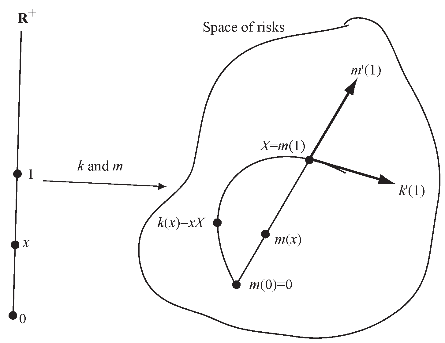
Figure 2.
Schematic of the Kalkbrener-Meyers example, using the sphere to illustrate the more complex space .
Figure 2.
Schematic of the Kalkbrener-Meyers example, using the sphere to illustrate the more complex space .
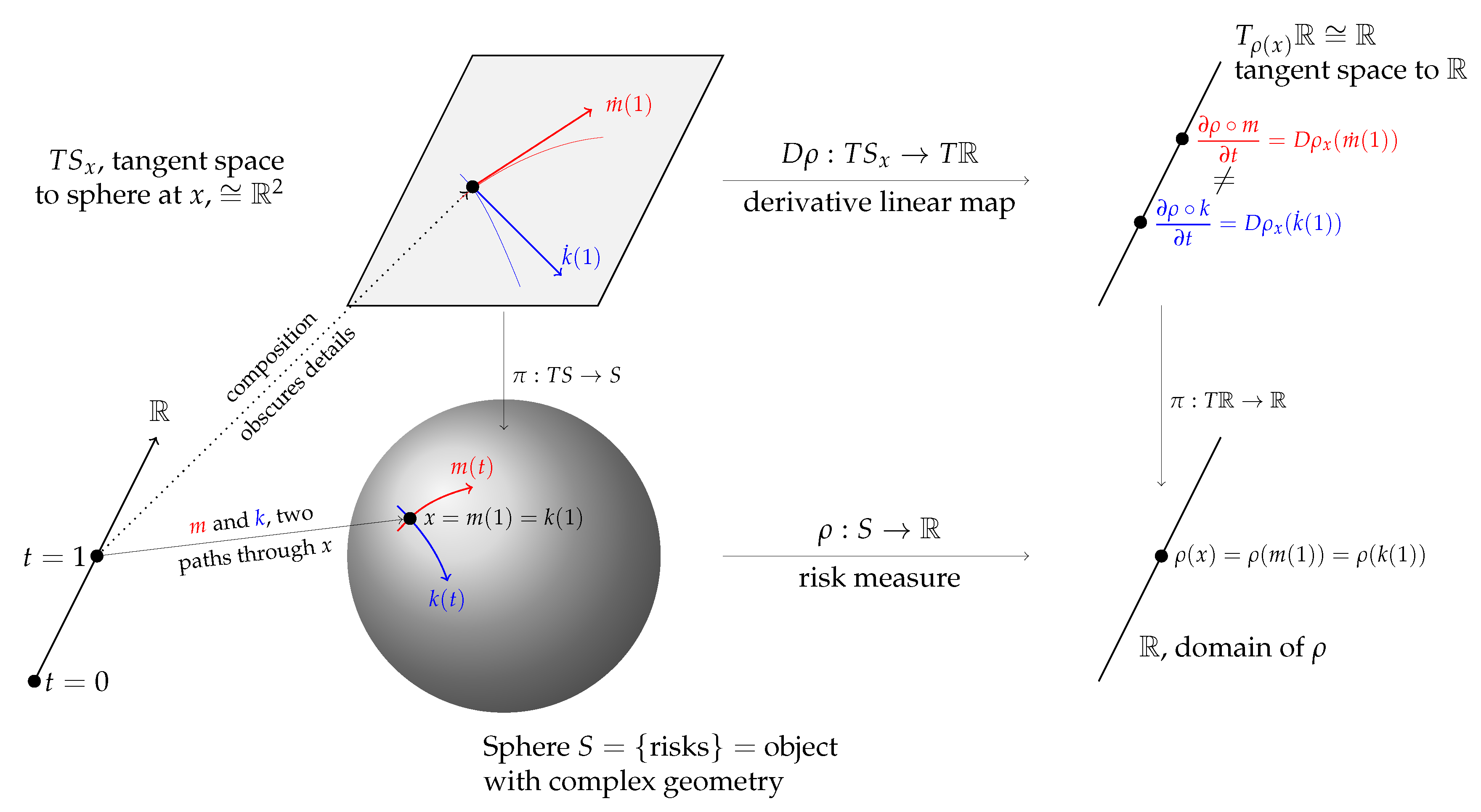
Figure 3.
Illustration of the difference between and for Z a standard normal as .

Figure 4.
Theoretical distribution of scaled aggregate losses with no parameter or structure uncertainty and Poisson frequency.
Figure 4.
Theoretical distribution of scaled aggregate losses with no parameter or structure uncertainty and Poisson frequency.

Figure 5.
Theoretical distribution envelope of scaled aggregate losses with a gamma mixed Poisson frequency with mixing variance .
Figure 5.
Theoretical distribution envelope of scaled aggregate losses with a gamma mixed Poisson frequency with mixing variance .
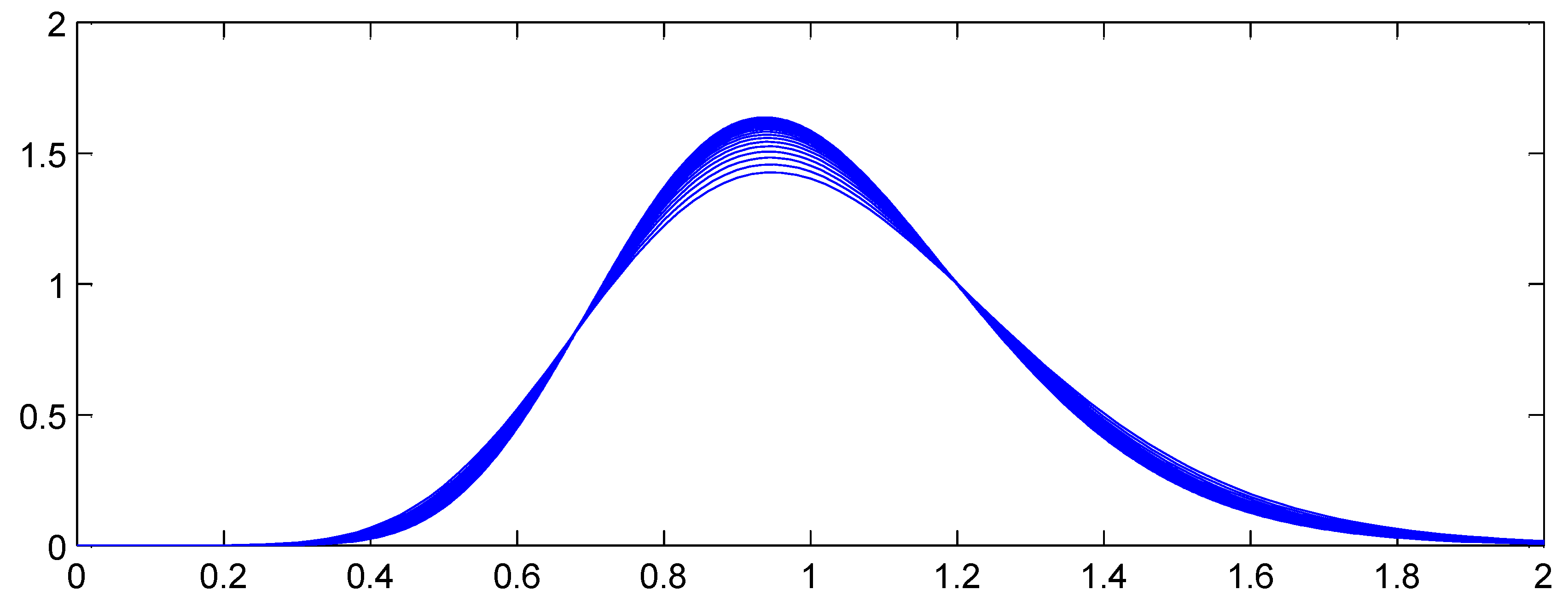
Figure 6.
The relationship between raw loss ratio volatility, measured as coefficient of variation of loss ratios, and premium volume, using data from accident years 1993–2004. Each inset graph plots the same data on a log/log scale, showing that the volatility continues to decrease materially for premium volumes in the $100Ms. The total line is distorted by changing mix of business by volume; the largest companies are dominated by private passenger auto liability which is the lowest volatility line.
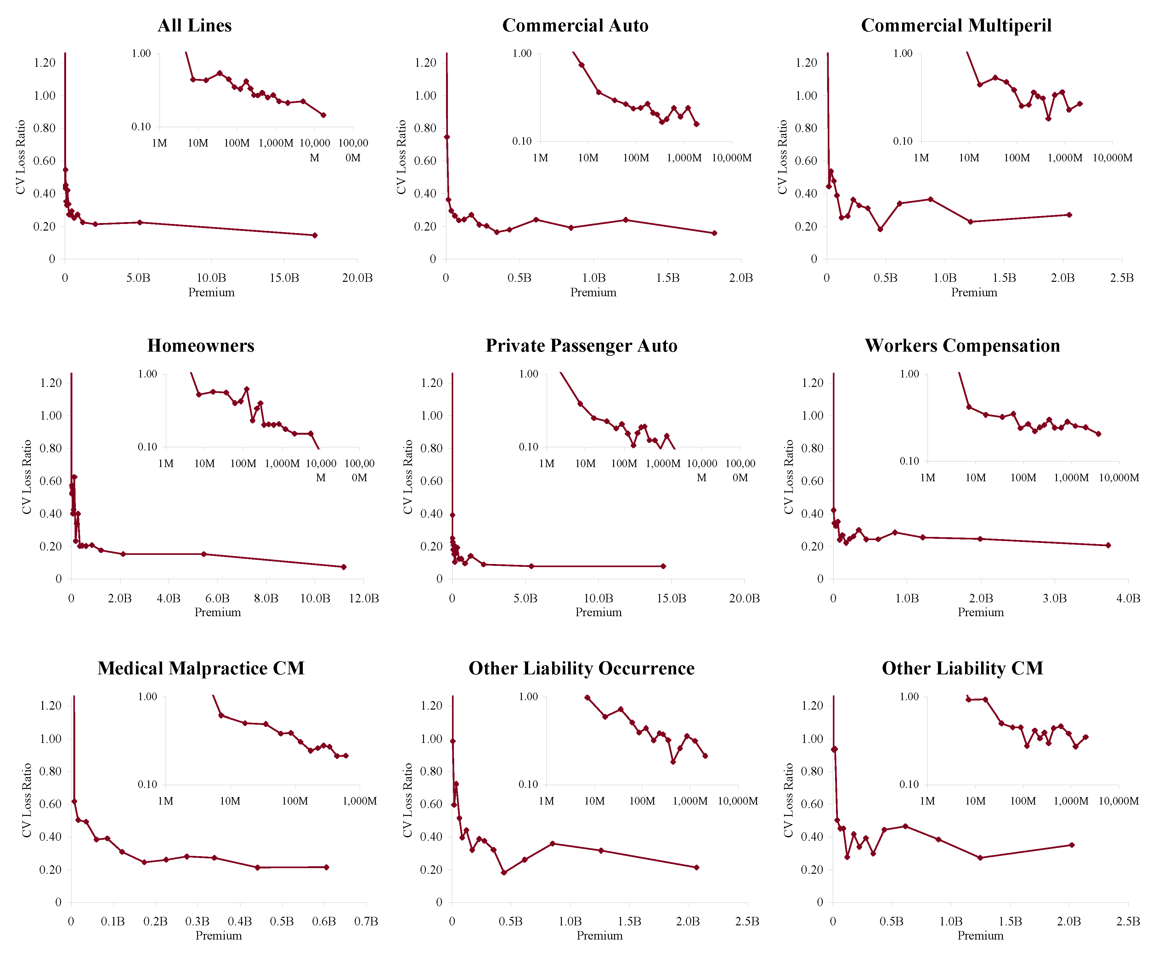
Figure 7.
Adjusted analysis of variance (ANOVA) for commercial auto, commercial multiperil and homeowners.
Figure 7.
Adjusted analysis of variance (ANOVA) for commercial auto, commercial multiperil and homeowners.

Figure 8.
Adjusted ANOVA for medical malpractice claims made and other liability claims made and occurrence.
Figure 8.
Adjusted ANOVA for medical malpractice claims made and other liability claims made and occurrence.

Figure 9.
Adjusted ANOVA for private passenger auto liability and workers compensation.
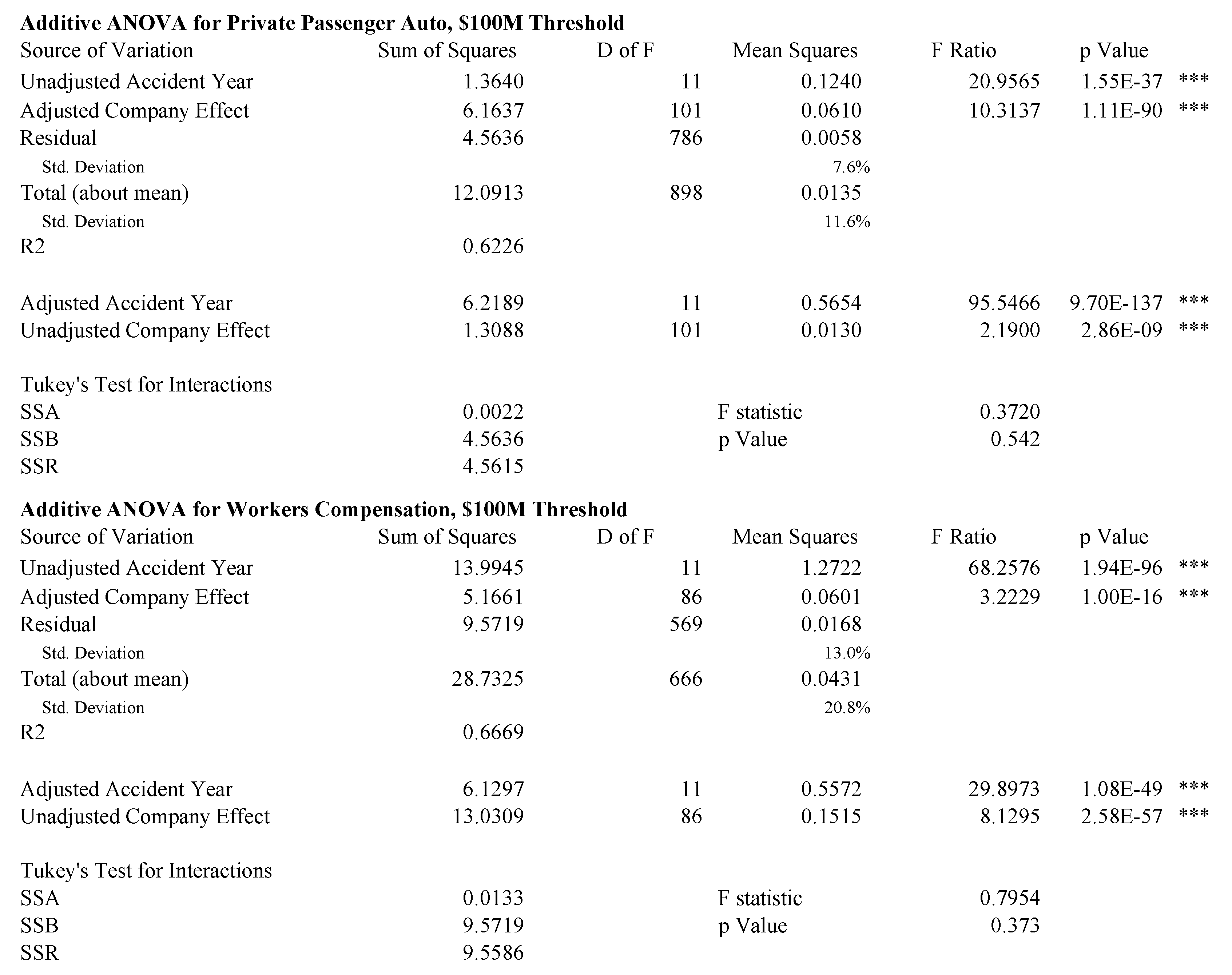
Figure 10.
Left plot shows the loss ratio volatility by line for companies writing $100M or more premium each year based on Schedule P accident year ultimate booked gross loss ratios, from 1993–2004. The graph shows the effect of adjusting the loss ratio for an accident year pricing effect, a company effect, and both effects (i.e., Res1-4). The right hand plot shows the differential impact of the pricing effect and company effect by line. Each bar shows the increase in volatility of the unadjusted loss ratios compared to the adjusted.

Figure 11.
Commercial auto liability (top four plots) and commercial multiperil volatility (bottom four plots). Note 9/11 loss effect in the lower-left plot. See text for a description of the plots.
Figure 11.
Commercial auto liability (top four plots) and commercial multiperil volatility (bottom four plots). Note 9/11 loss effect in the lower-left plot. See text for a description of the plots.

Figure 12.
Homeowners (top four plots) and medical malpractice claims made volatility (bottom four plots). Note the 2004 homowners catastrophe losses. See text for a description of the plots.
Figure 12.
Homeowners (top four plots) and medical malpractice claims made volatility (bottom four plots). Note the 2004 homowners catastrophe losses. See text for a description of the plots.

Figure 13.
Other liability claims made (top four plots) and occurrence volatility (bottom four plots). See text for a description of the plots.
Figure 13.
Other liability claims made (top four plots) and occurrence volatility (bottom four plots). See text for a description of the plots.

Figure 14.
Private passenger auto liability (top four plots) and workers compensation volatility (bottom four plots). Note vertical scale on private passenger auto loss ratios and the visibly higher volatility of premium than loss in the lower left hand plot. See text for a description of the plots.

Figure 15.
Coefficient of variation of loss ratio by premium volume for private passenger auto liability, computed using bucketed for .
Figure 15.
Coefficient of variation of loss ratio by premium volume for private passenger auto liability, computed using bucketed for .
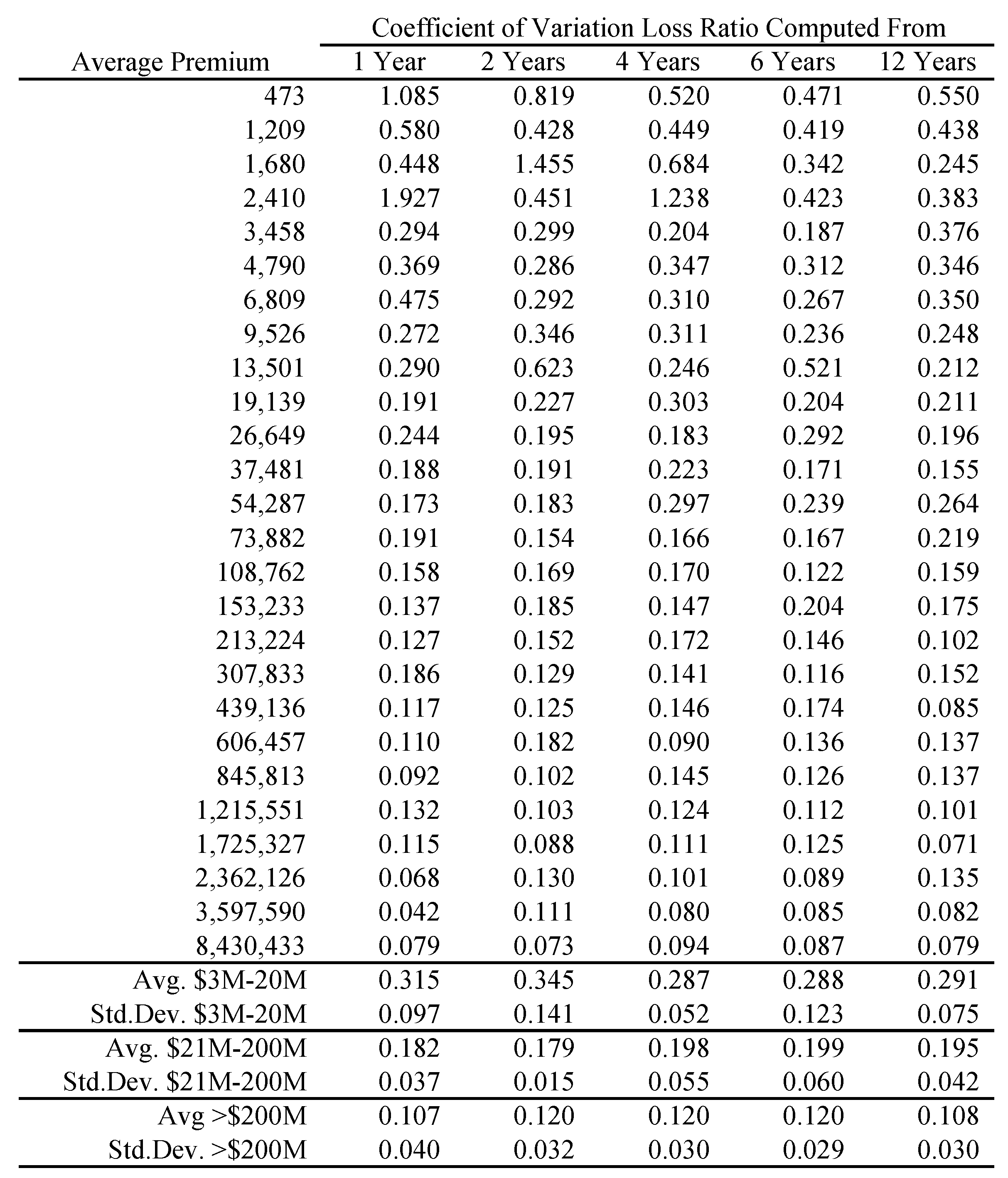
Figure 16.
Fit of to volatility by volume, , for homeowners, private passenger auto and commercial auto. Left hand plot shows data based on a single year ; right hand plot shows the same data for .
Figure 16.
Fit of to volatility by volume, , for homeowners, private passenger auto and commercial auto. Left hand plot shows data based on a single year ; right hand plot shows the same data for .
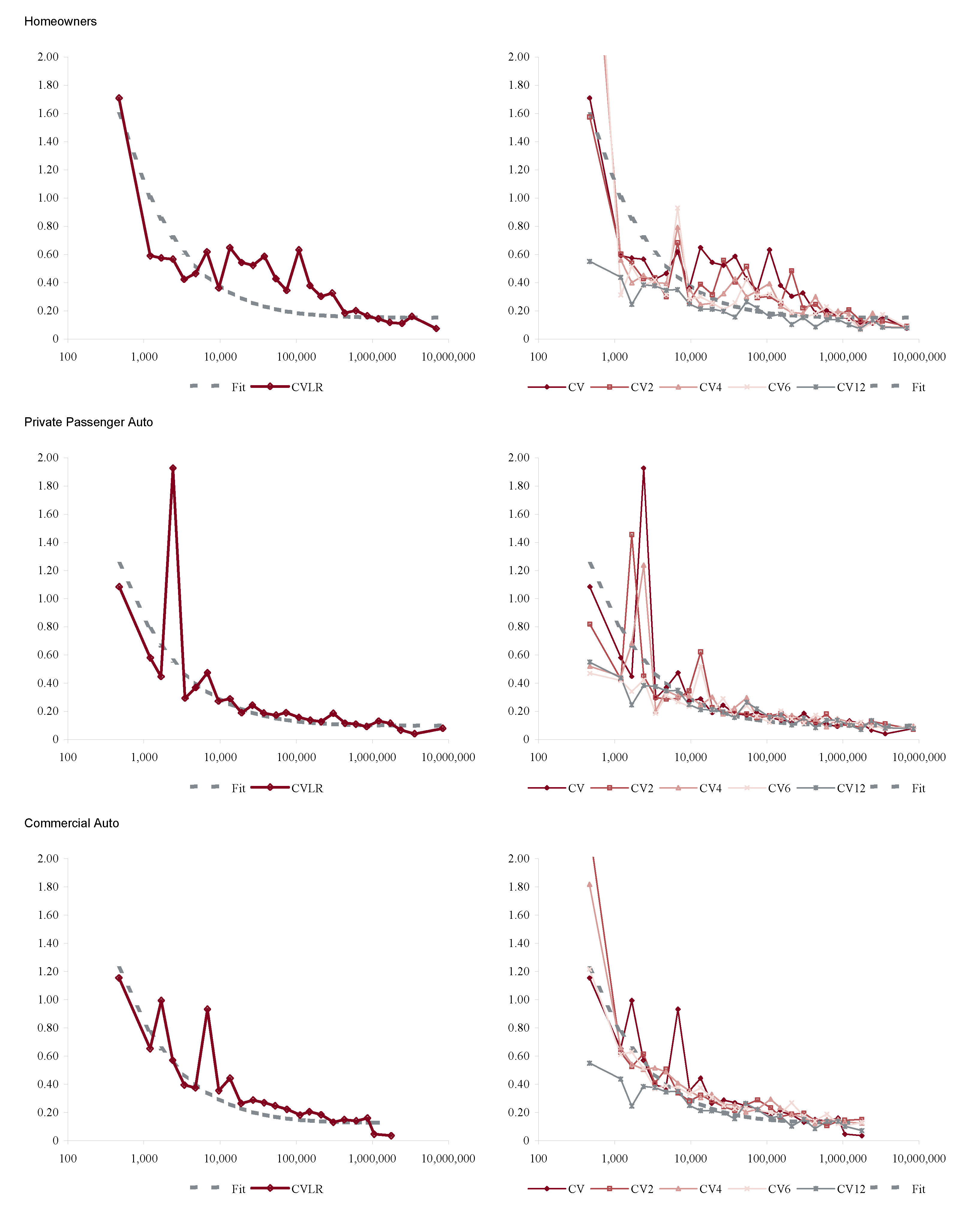
Figure 17.
Fit of to volatility by volume, , for workers compensation, commercial multiperil and other liability occurrence. Left hand plot shows data based on a single year ; right hand plot shows the same data for .
Figure 17.
Fit of to volatility by volume, , for workers compensation, commercial multiperil and other liability occurrence. Left hand plot shows data based on a single year ; right hand plot shows the same data for .


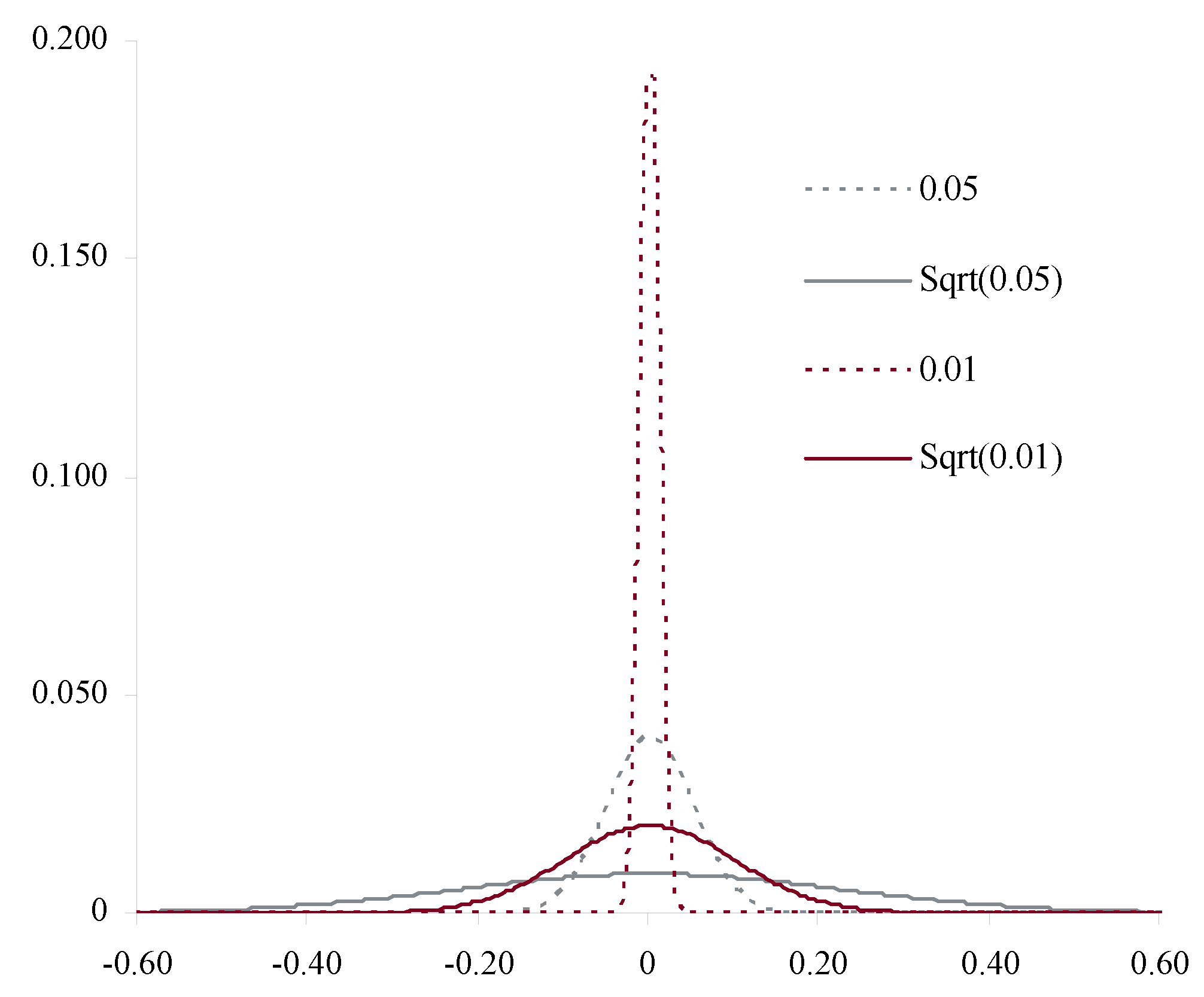
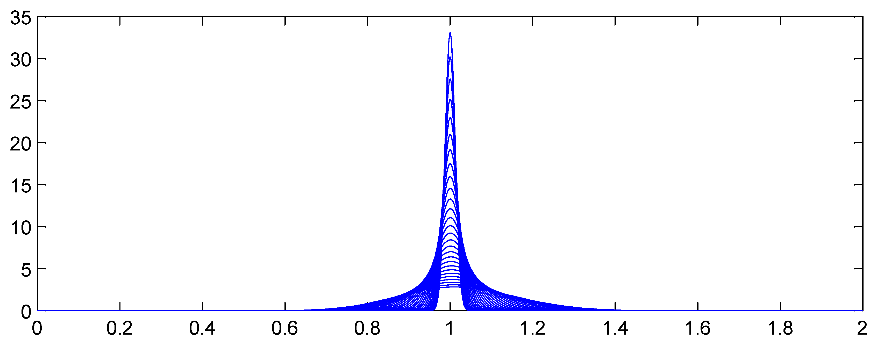
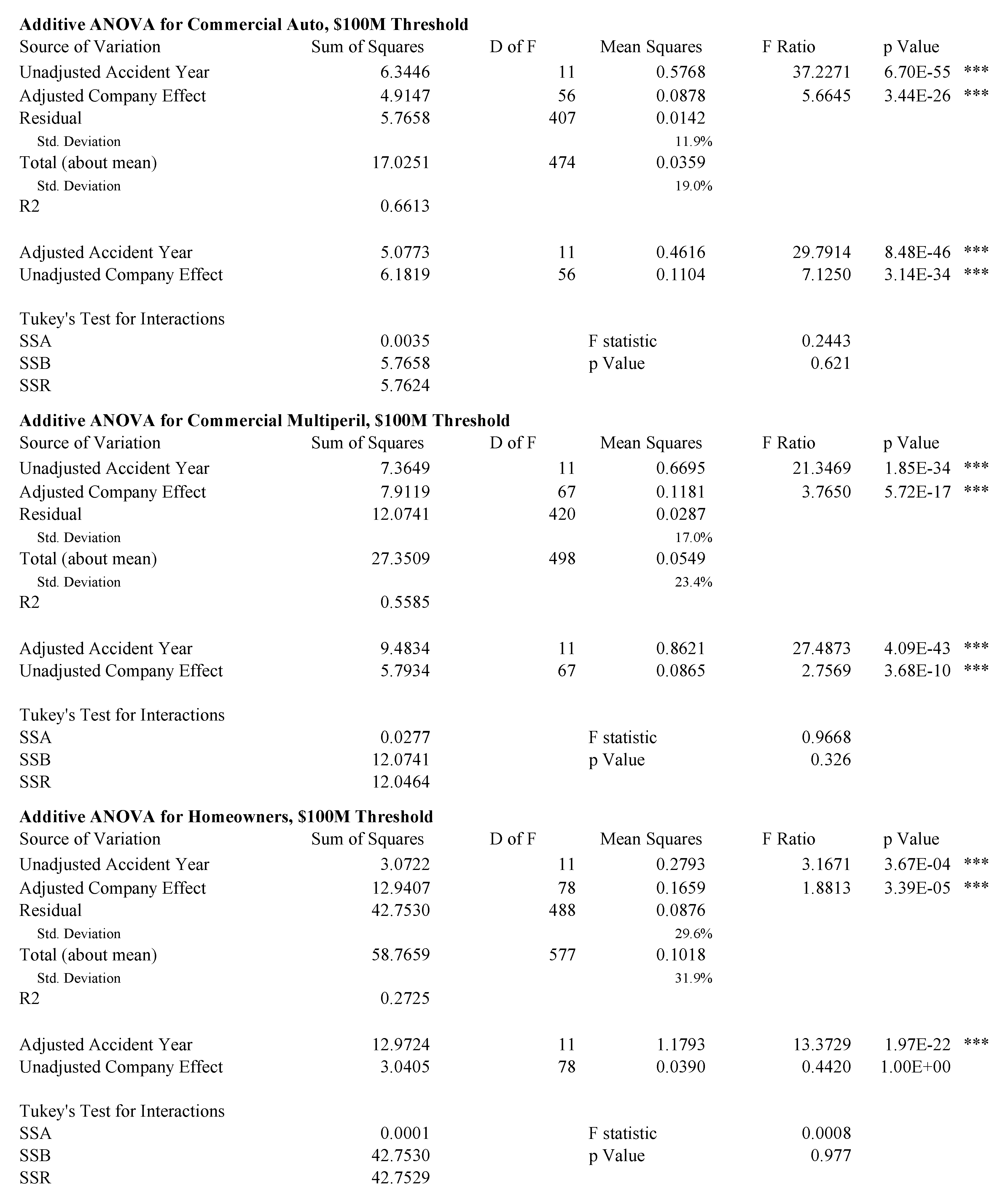
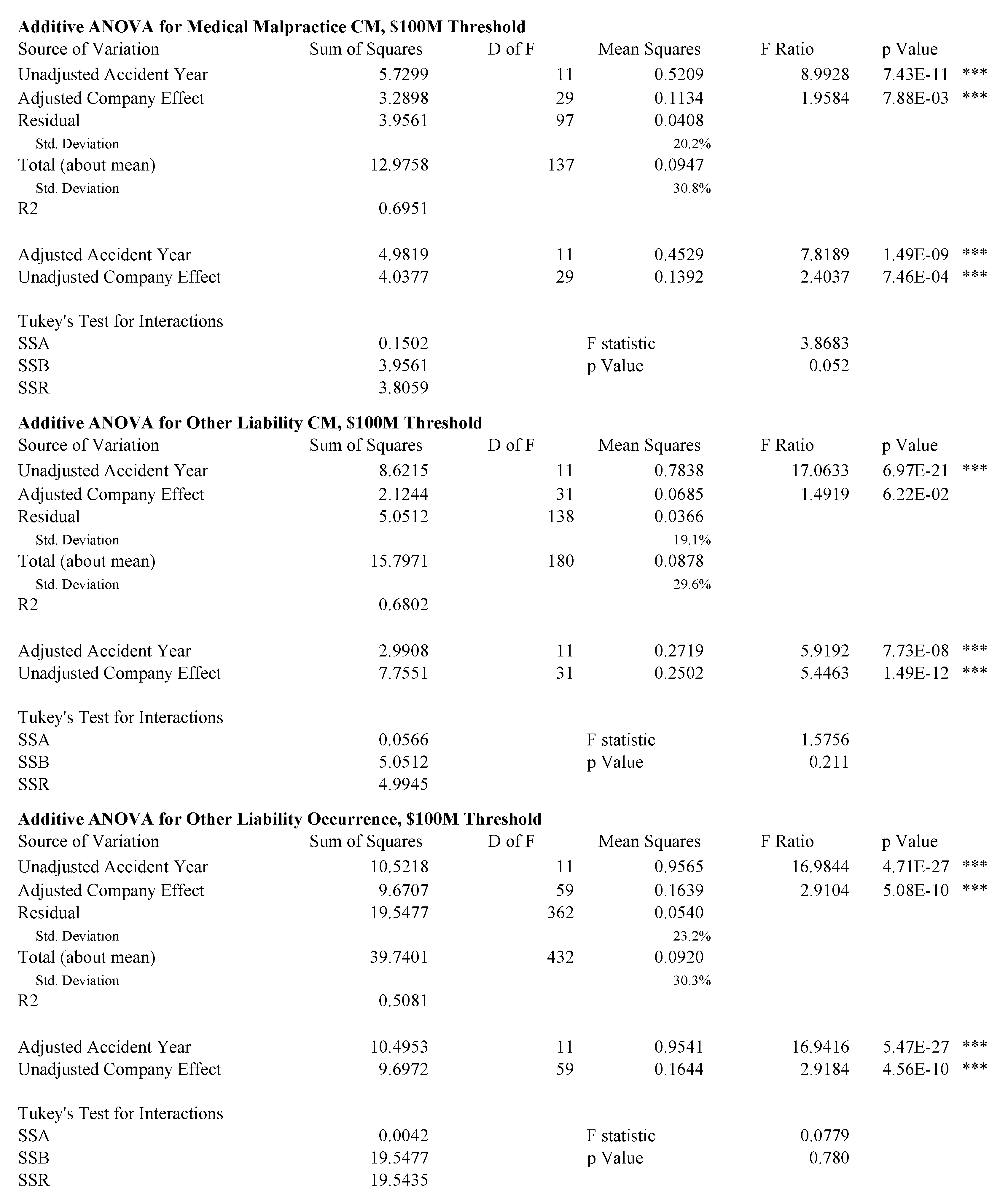
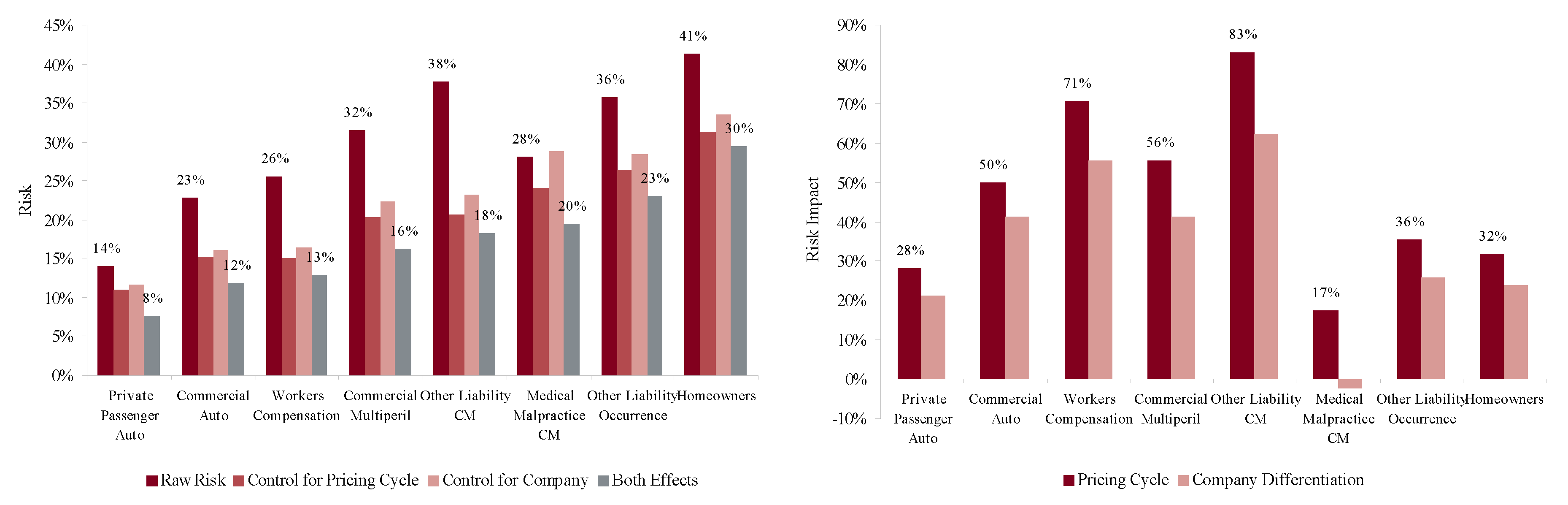
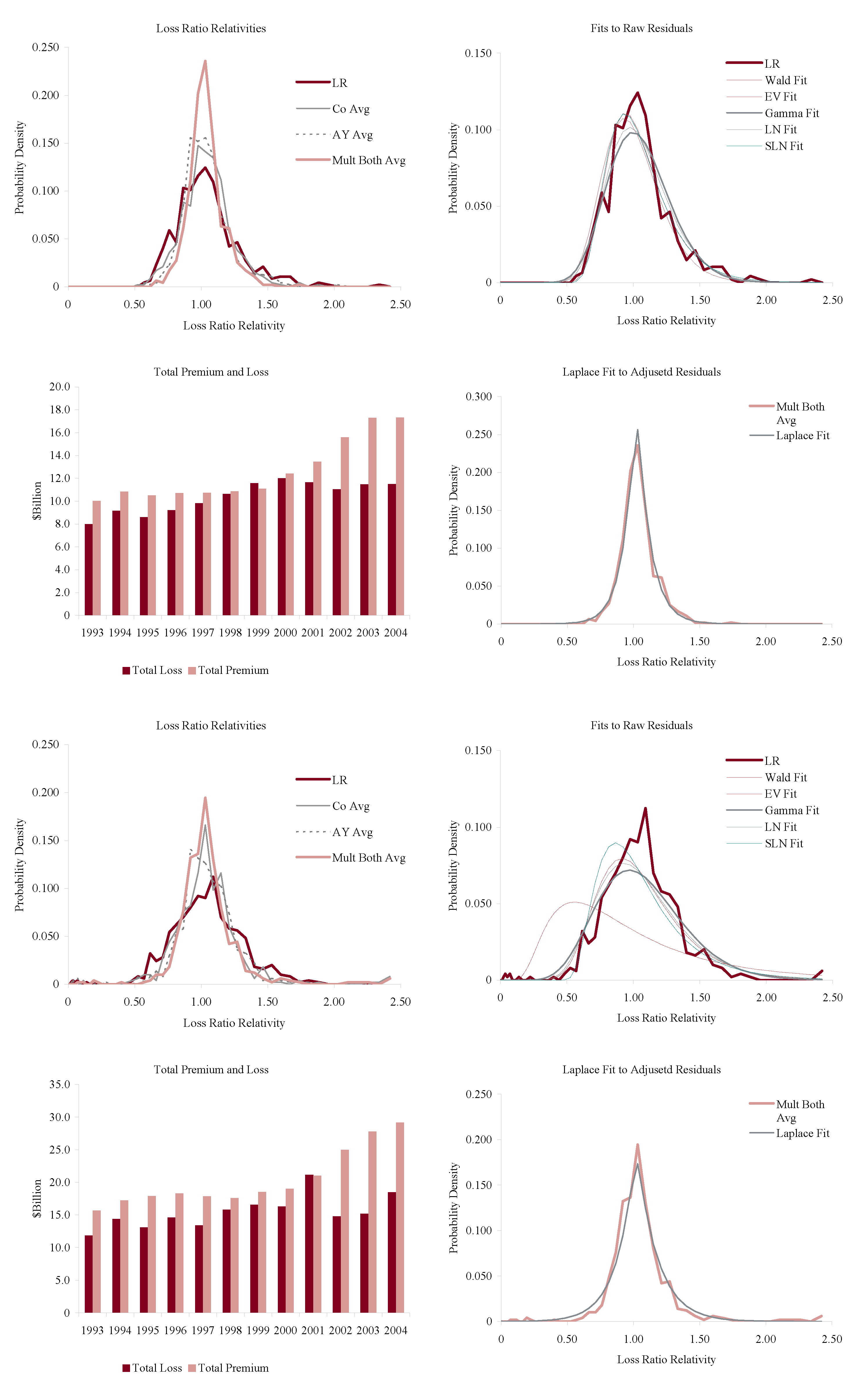
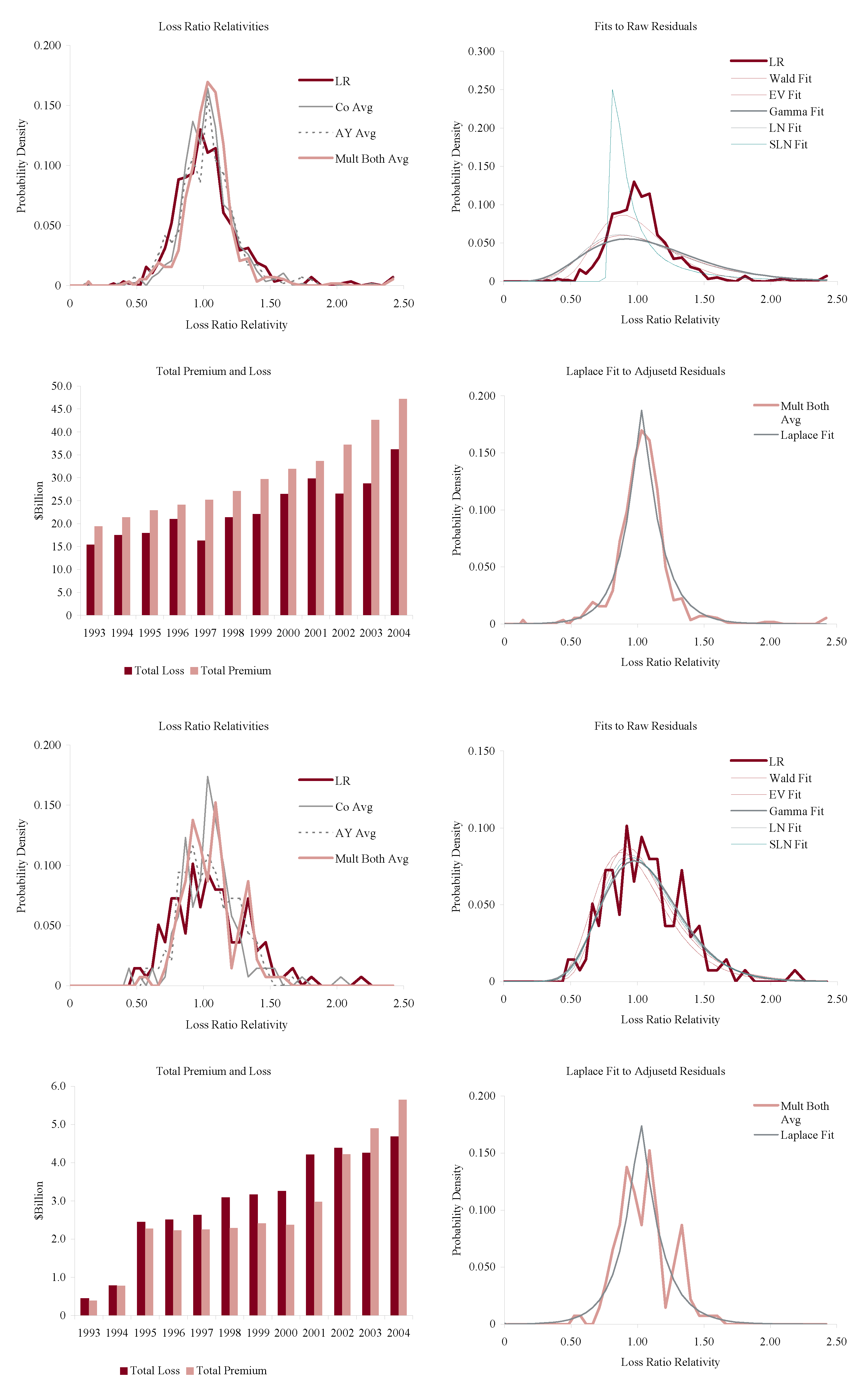
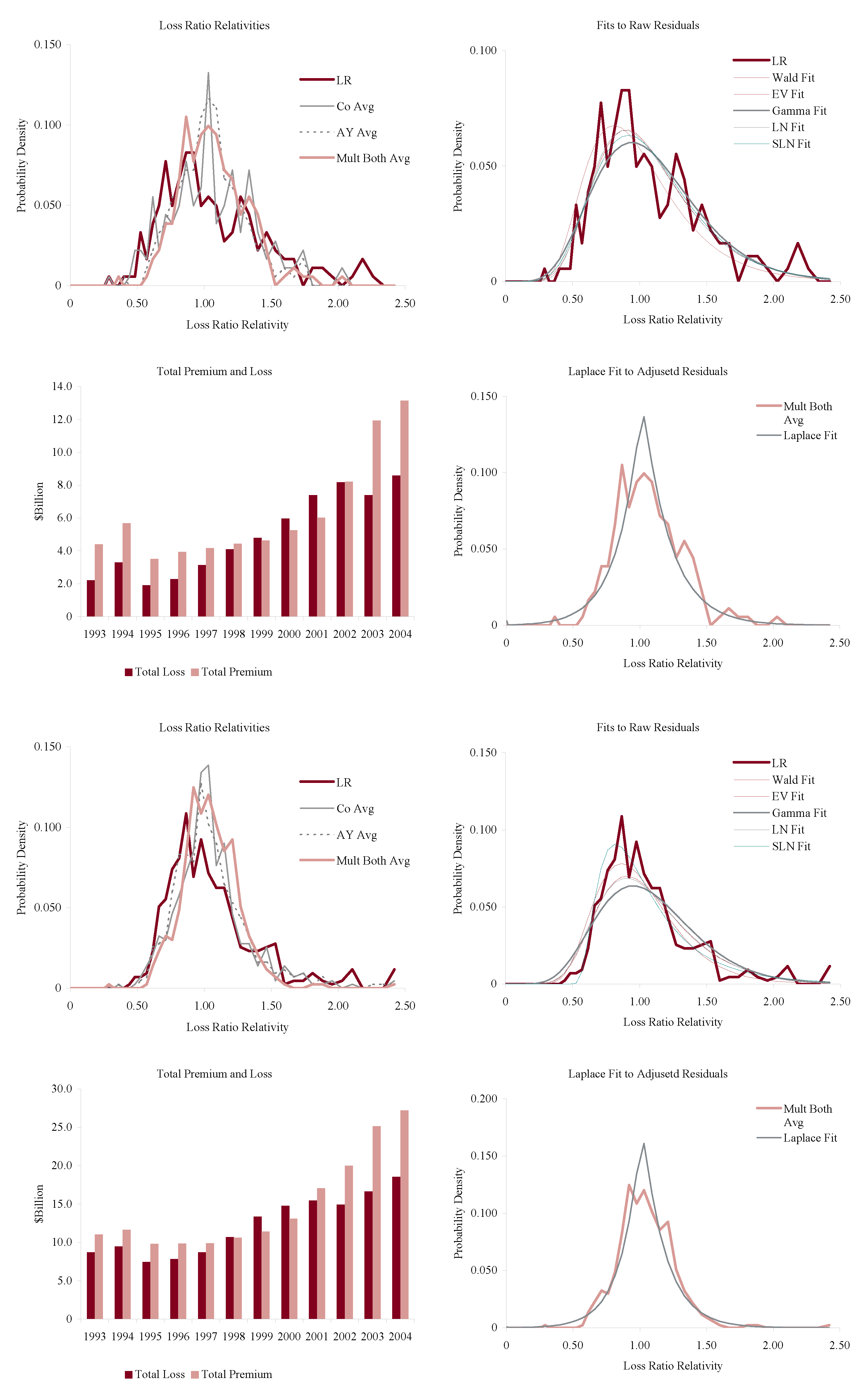
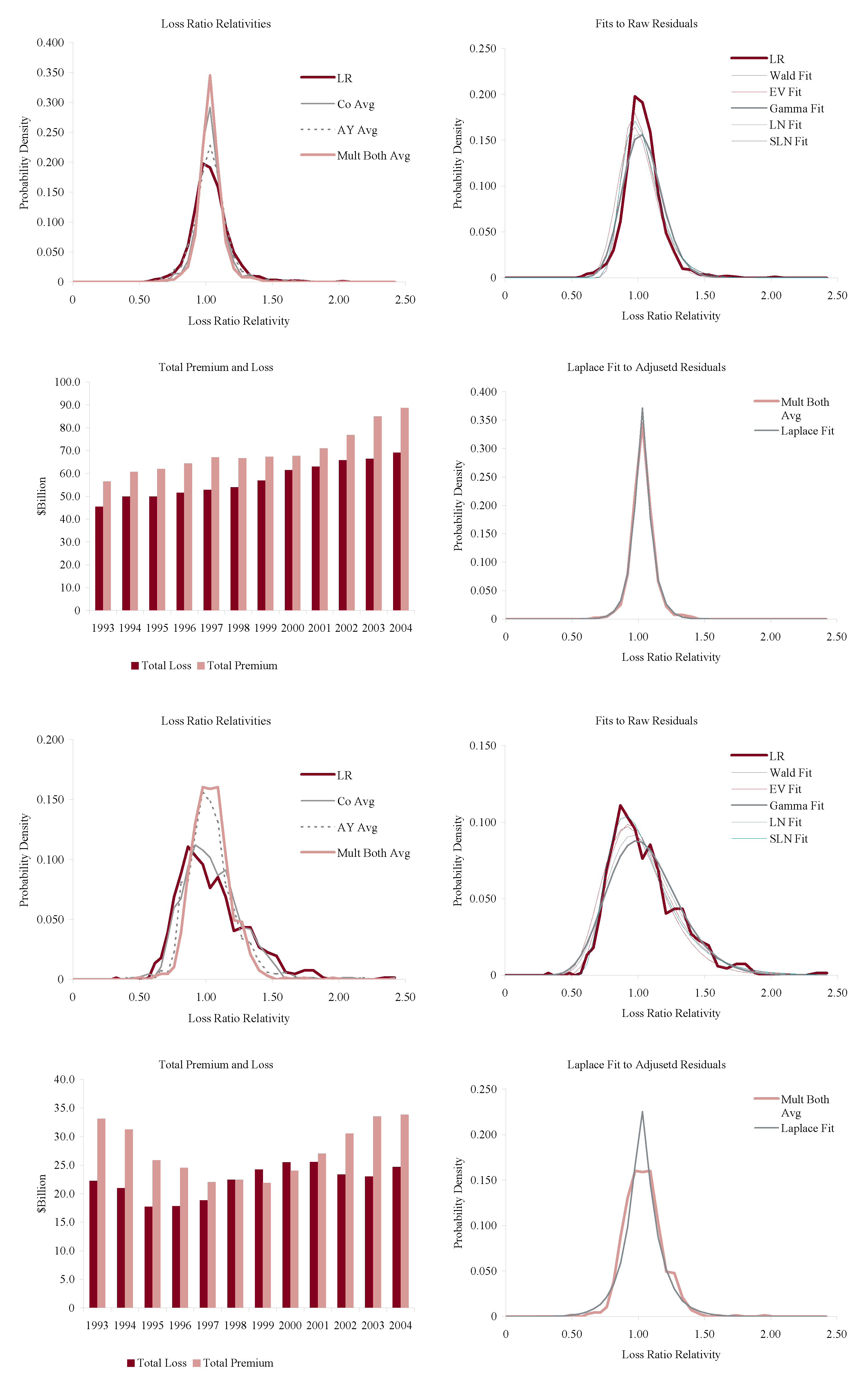
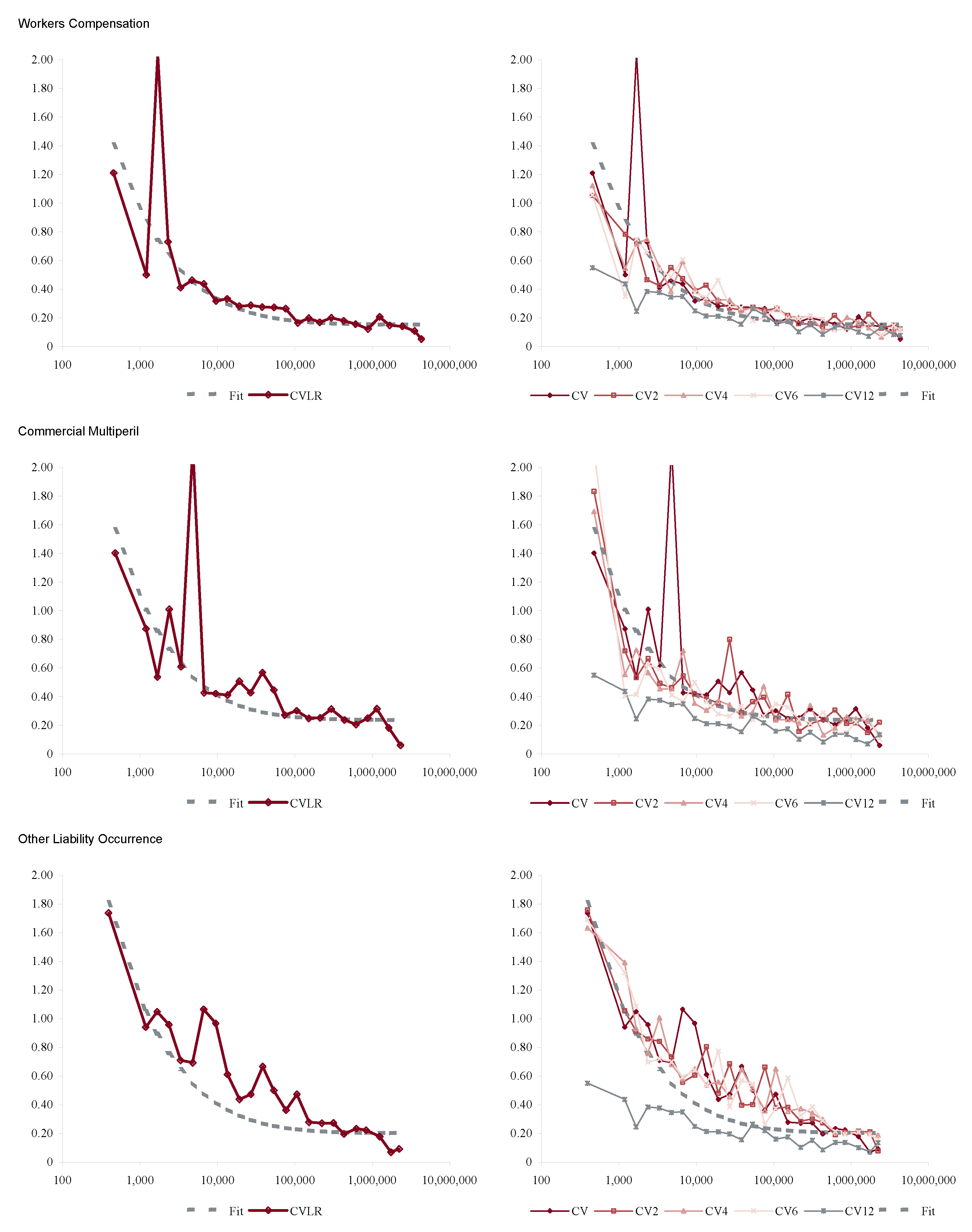
Table 1.
Variance of IM1-4 and AM.
| Model | Variance | Diversifying | ||
|---|---|---|---|---|
| IM1: | Yes | Yes | ||
| IM2: | No | Yes | ||
| IM3: | No | No | ||
| IM4: | No | No | ||
| AM1: | Const. | Yes | ||
In IM4, .
Table 2.
Possible characterizations of a ray in .
| Characterization of Ray | Required Structure on |
|---|---|
| is the shortest distance between and | Notion of distance in , differentiable manifold |
| , constant velocity, no acceleration | Very complicated on a general manifold. |
| , . | Vector space structure |
| Can add in domain and range, semigroup structure only. |
Table 3.
Characteristics of Various Lines of Insurance
| Insurance Line | Heterogeneity | Regulation | Limits | Cycle | Cats |
|---|---|---|---|---|---|
| Personal Auto | Low | High | Low | Low | No |
| Commercial Auto | Moderate | Moderate | Moderate | High | No |
| Workers Compensation | Moderate | High | Statutory | High | Possible |
| Medical Malpractice | Moderate | Moderate | Moderate | High | No |
| Commercial Multi-Peril | Moderate | Moderate | Moderate | High | Moderate |
| Other Liability Occurrence | High | Low | High | High | Yes |
| Homeowners Multi-Peril | Moderate | High | Low | Low | High |
| Other Liability Claims Made | High | Low | High | High | Possible |
| Abbreviation | Parameters | Distribution | Fitting Method |
|---|---|---|---|
| Wald | 2 | Wald (inverse Gaussian) | Maximum likelihood |
| EV | 2 | Frechet-Tippet extreme value | Method of moments |
| Gamma | 2 | Gamma | Method of moments |
| LN | 2 | Lognormal | Maximum likelihood |
| SLN | 3 | Shifted lognormal | Method of moments |
Table 5.
Comparison of risk factors with Solvency II premium risk factors.
| Dimension | Actuarial Geometry | Solvency II |
|---|---|---|
| Time horizon | to ultimate | one year |
| Catastrophe risk | included | excluded |
| Size of company | large | average |
Table 6.
Coefficient of variation of gross loss ratio, Source: Aon Benfield Insurance Risk Study, 7th Edition, used with permission.
Table 6.
Coefficient of variation of gross loss ratio, Source: Aon Benfield Insurance Risk Study, 7th Edition, used with permission.
| Line | 1st Edition | 7th Edition | Change |
|---|---|---|---|
| Private Passenger Auto | 14% | 14% | 0% |
| Commercial Auto | 24% | 24% | 0% |
| Workers’ Compensation | 26% | 27% | 1% |
| Commercial Multi Peril | 32% | 34% | 2% |
| Medical Malpractice: Claims-Made | 33% | 42% | 9% |
| Medical Malpractice: Occurrence | 35% | 35% | 0% |
| Other Liability: Occurrence | 36% | 38% | 2% |
| Special Liability | 39% | 39% | 0% |
| Other Liability: Claims-Made | 39% | 41% | 2% |
| Reinsurance Liability | 42% | 67% | 25% |
| Products Liability: Occurrence | 43% | 47% | 4% |
| International | 45% | 72% | 27% |
| Homeowners | 47% | 48% | 1% |
| Reinsurance: Property | 65% | 85% | 20% |
| Reinsurance: Financial | 81% | 93% | 12% |
| Products Liability: Claims-Made | 102% | 100% | −2% |
© 2017 by the author. Licensee MDPI, Basel, Switzerland. This article is an open access article distributed under the terms and conditions of the Creative Commons Attribution (CC BY) license (http://creativecommons.org/licenses/by/4.0/).
Share and Cite
MDPI and ACS Style
Mildenhall, S.J. Actuarial Geometry. Risks 2017, 5, 31. https://doi.org/10.3390/risks5020031
AMA Style
Mildenhall SJ. Actuarial Geometry. Risks. 2017; 5(2):31. https://doi.org/10.3390/risks5020031
Chicago/Turabian StyleMildenhall, Stephen J. 2017. "Actuarial Geometry" Risks 5, no. 2: 31. https://doi.org/10.3390/risks5020031
Note that from the first issue of 2016, this journal uses article numbers instead of page numbers. See further details here.