
Bubbles, Blind-Spots and Brexit

1
School of Computing Mathematics and Digital Technology, Manchester Metropolitan University, John Dalton Building, Chester Street, Manchester M1 5GD, UK
2
Sheffield University Management School, Conduit Road, Sheffield S10 1FL, UK
*
Author to whom correspondence should be addressed.
Risks 2017, 5(3), 37; https://doi.org/10.3390/risks5030037
Submission received: 28 April 2017
/
Revised: 12 July 2017
/
Accepted: 13 July 2017
/
Published: 18 July 2017
(This article belongs to the Special Issue The implications of Brexit)
Abstract
:In this paper we develop a well-established financial model to investigate whether bubbles were present in opinion polls and betting markets prior to the UK’s vote on EU membership on 23 June 2016. The importance of our contribution is threefold. Firstly, our continuous-time model allows for irregularly spaced time series—a common feature of polling data. Secondly, we build on qualitative comparisons that are often made between market cycles and voting patterns. Thirdly, our approach is theoretically elegant. Thus, where bubbles are found we suggest a suitable adjustment. We find evidence of bubbles in polling data. This suggests they systematically over-estimate the proportion voting for remain. In contrast, bookmakers’ odds appear to show none of this bubble-like over-confidence. However, implied probabilities from bookmakers’ odds appear remarkably unresponsive to polling data that nonetheless indicates a close-fought vote.
1. Introduction
Following a referendum held on 23 June 2016 the UK voted in favour of leaving the EU by a margin of 51.9–48.1%. Though there are suggestions that such euroscepticism had been increasing in recent years (Tarran 2016) it was generally believed that there was popular British support for EU membership. In many ways a vote for Brexit (“Britain exit”) in favour of Bremain (“Britain remain”) was a shock result. Inter alia the final result ran counter to the available data on bookmakers’ odds and opinion polls—though opinion polls did suggest a closely fought contest. There are therefore two natural questions of interest. Firstly, to what extent could Brexit have been predicted? Secondly, were pollsters and bookmakers over-confident1 or simply blind to some of the available evidence?
In this paper we restrict to publicly available information from opinion polls and bookmakers’ odds. Both are natural things to look at and both have been previously studied in the literature (see, e.g., Ford et al. 2016; Erikson and Wleizen 2012). Amidst a mixed forecasting record (Leigh and Wolfers 2006; Vaughan Williams and Reade 2016) it is important to recognise that both data sources may have their limitations. The accuracy of polling has long been questioned (see, e.g., Hyman 1944). Social pressures mean survey respondents often over-report their likelihood of voting (Whiteley 2016). Relatedly, survey respondents may also be reluctant to admit their true voting intentions to interviewers if they perceive that their choice is unpopular. In the UK this has led to the phenomenon of the “shy Tory” with polls systematically under-estimating the true level of support for the Conservative Party (Whiteley 2016). Similarly, in the United States the so-called Bradley Effect has caused polls to over-estimate the level of support for non-white candidates (Payne 2010). Based on the 2016 US presidential election other limitations to working with polling data include concern over non-response rates—especially differential non-response—whereby voters fail to participate in polls if they perceive that their side is performing badly. As is the case with opinion polls bookmakers’ odds may not faithfully reflect the true underlying probabilities. Shin (1993) proposed a theoretical model based on the assumption that bookmakers quote odds that maximise their expected profit in the presence of uninformed traders and a known proportion of insider traders. From a practical perspective Štrumbelj (2014) reports significant variations in the accuracy of bookmakers’ forecasts on sports’ betting markets.
In view of the above we follow a complex systems approach to forecasting that has previously proved very successful in finance (Sornette 2003). Complex systems offer a natural description of the problem at hand and the difficult-to-foresee macroscopic or emergent properties that can result from the interactions between the microscopic components of the system—here individual voters (see below). Inter alia complex systems lie at the heart of a so-called wisdom of crowds effect in political forecasting (Murr 2016). Further, the analogy between financial markets and elections is compelling.
Complex systems occur when a system is composed of many microscopic parts that interact with each other. These interactions combine to generate surprising macroscopic or emergent properties that typically display behaviour that is a lot richer than the behaviour of individual system components in isolation. This feature underpins the modelling approach taken here. Complex systems have been found in many different systems in both natural and social sciences (see, e.g., Sornette 2003, 2006). Examples of complex social systems include financial and economic crashes, outbreaks of social unrest, engineering structures and traffic systems (Sornette 2003). An alternative listing including applications as diverse as politics, financial markets, popular music and fashion is given in Prechter (1999).
The analogy between bubbles and crashes in financial markets and political votes (elections and referenda) is striking. Firstly, both events can clearly be categorised as complex systems problems. A multitude of factors clearly influence the outcomes of both systems. Further, the behaviour of both systems emerges as a result of the microscopic interactions between economic agents (financial markets) and constituents/ voters (political systems). A powerful social element underpins both settings (see, e.g., Kindelberger and Aliber 2005; Whiteley 2016). The effects can be dramatic and can be extended to include psychological factors and herding (Prechter 1999). Beyond a purely qualitative comparison attempts have been made to use the stock market, as a barometer of collective social mood, to predict elections (Prechter et al. 2012). Further, economic models of voting patterns are well established within the mainstream literature (see, e.g., Leigh and Wolfers 2006). As far as Brexit is concerned one possible predictor might include the US Dollar-GBP currency pair (Spence and Wallace 2016) or their associated derivatives markets (Clark and Amen 2017). (Similarly, it is thought that fluctuations in the US Dollar-Mexican Peso currency pair may also have predictive power for the recent US presidential election.) Here, we take a different approach. Using the theory of financial bubbles (Fry 2012; Johansen et al. 2000) we test to see if bookmakers’ odds and opinion polls systematically over-price the probability of a remain vote in the EU referendum.
The contribution of our paper is as follows. Based on the theory of financial bubbles we develop a model for over-confidence in opinion polls and betting odds. Here, over-confidence manifests itself in the sense that, collectively, market participants are over-precise in their assessments of the underlying price risk (see Section 3). Our approach copes well with known features of polling data such as irregularly-spaced time series. Further, the elegance of our approach is such we can easily make adjustments for the size of the distortion found. Moreover, our model is also easier to apply in practice than other economic and financial models of voting behaviour (see Section 2). It is found that both opinion polls and bookmakers’ odds under-estimate the probability of a Brexit vote. Making an adjustment for over-confidence our out-of-sample forecast is a vote for Brexit by a margin of 50.6–49.4%. Even without this adjustment raw opinion poll data suggests a very close vote—something Bookmakers’ odds appear almost blind to.
The layout of this paper is as follows. Section 2 discusses related literature. Section 3 discusses the probability model used. Section 4 analyses empirical data from opinion polls and bookmakers’ odds on the eve on the Brexit vote. Section 5 concludes and discusses the possibilities for further research. A separate empirical application to polling data from the 2014 Scottish Independence Referendum is discussed in an Appendix at the end of the paper.
2. Related Literature
2.1. Political Modelling
There are three core themes in the political modelling literature that our paper contributes to. These are the comparison of data from betting and prediction markets with opinion poll data, forecasting political events using opinion poll data and the use of economic and financial models—an issue of particular significance given the modelling approaches adopted in Section 3 and Section 4.
There is a long history of betting and prediction markets for political events (see, e.g., Rhode and Strumpf 2004). The use of prediction markets is now a whole subject in its own right with novel predictions being made in areas as diverse as Movie box-office receipts, Movie Oscar winners, the timing of scientific and technological breakthroughs, football World Cup matches, Formula One races and market research (Kou and Sobel 2004). As far as politics is concerned Kou and Sobel (2004) provide theoretical justification that prediction markets should out-perform polls if polls are included in the information set of market participants. Rothschild (Rothschild 2009) finds that de-biased prediction markets out-perform de-biased polls. Betting markets also have the advantage that publicly-known events can be immediately incorporated into market prices but may take several days to be incorporated into polls. It is widely believed that betting markets should produce better forecasts than opinion polls. In Leigh and Wolfers (2006) it is suggested that prediction markets may produce less volatile forecasts than opinion polls. Similarly, Vaughan Williams and Reade (2016) report that prediction markets provide more precise forecasts than opinion polls. Berg et al. (2008) find that prediction markets out-perform polls—especially over the longer term.
Beyond the comparison with betting markets using polling data to make political forecasts is of fundamental importance in its own right. Theoretical advantages of betting markets are predicated on the assumption, which may or may not hold in the real world, that polling data is actively studied by market participants (Kou and Sobel 2004). There are even occasions when opinion polls marginally out-perform prediction markets (Erikson and Wleizen 2012). In Erikson and Wleizen (2008) de-biased opinion polls out-perform raw prediction markets. In recent applications Fisher (2016) uses data from opinion polls coupled with individual constituency level information to forecast the 2015 British general election. In a similar vein Ford et al. (Ford et al. 2016) develop a hierarchical model to predict the 2015 British general election using data from opinion polls. However, it is important to note that in both cases there is some discrepancy between the forecasts made and the observed electoral results.
Though the links between politics and the wider economy is much discussed by commentators and academics alike (see, e.g., Herron et al. 1999) economic models of voting behaviour appear to be relatively under-explored (Leigh and Wolfers 2006). Important limitations include the complexity of economic models and the availability of data—especially at higher frequencies. The economic literature includes work on the political partisanship of election winners and economic conditions (Alesina and Roubini 1992), political business cycle theories whereby incumbent politicians manipulate the economy to maximise their prospects of re-election (Rogoff 1990) and the relationship between stock prices and the expected outcomes of national elections (Herron et al. 1999). Leigh and Wolfers (2006) use economic data on unemployment, inflation, GDP growth, wage growth and wars to try and predict the results of Australian elections.
Beyond economic models of voting behaviour several works hint at close connections between political systems and financial markets. This serves as direct motivation for the modelling approaches undertaken in Section 3 and Section 4. Lewis-Beck et al. (2016) use a combination of polling data and economic models to predict the 2015 British general election. Lewis-Beck et al. (Lewis-Beck et al. 2016) also refer to the importance of leader image in elections—an observation that brings to mind Keynes’ famous “beauty contest” description of stock market investment together with other self-fulfilling prophecies and behavioural factors that may affect financial markets (see, e.g., Sornette 2003). In Herron et al. (1999) the prices of defence and pharmaceutical stocks are shown to vary according to prediction-market-based measures of presidential candidates’ standing—with the electoral results in question having clear implications for firms in both sectors. On a related theme Oehler et al. (2017) find evidence of relatively low levels of abnormal stock returns following the Brexit referendum with firms which have a higher degree of internationalisation being less severely affected. In Prechter et al. (2012) the stock market is identified as having more influence upon presidential re-election outcomes than other economic variables such as GDP, inflation and employment. Similarly, in Prechter (1999) heavy defeats and large victories for the incumbent president are associated with major bear and bull markets respectively.
2.2. Bubbles and Crashes in Financial Markets
Kindelberger and Aliber (2005) describe bubbles as a sharp rise in asset prices - with the initial rise generating expectations of further rises and attracting new buyers. This influx of new investors may be one of the key features of bubbles hidden behind the mass panic and manias (Zeira 1997). These new investors are generally speculators interested in profiting from trading in the asset rather than the asset’s use or earning capacity. Excessive public expectations of future price rises thus cause prices to be temporarily elevated (Shiller 2005). These temporary price rises can neither be justified by changes in fundamentals nor by the asset’s anticipated cash flow. During such bubble episodes assets may be increasingly viewed as a purely tradable commodity that can be sold for profit (Kindelberger and Aliber 2005). A common misconception is that bubbles necessarily imply irrationality on the part of investors. However, rational expectations models were introduced by Blanchard and Watson (1982) to account for the possibility that asset prices may deviate from fundamental levels without assuming mass irrationality on the part of market participants. In Johansen et al. (2000) a representative investor is compensated for bearing the risk of a crash by the potential for large rewards. In alternative treatments of this model this is accompanied by a collective market over-confidence (see, e.g., Fry 2012).
Identifying bubbles in asset prices is challenging and the literature has yet to reach a consensus (see, e.g., Gürkaynak 2008). Protagonists of bubbles assume that prices were equal to fundamental values historically before a period of rapid growth. Opponents argue that observed prices may have been too low and that increasing prices may simply represent an adjustment to long-term equilibrium values. Whilst this view of bubbles—as a temporary increase above long-term fundamental values—makes a lot of sense there has been some debate regarding econometric mis-specifications of models for bubbles in the literature. Diba and Grossman (Diba and Grossman 1988) suggest that if stock prices and dividends are cointegrated—i.e., that there is a long term relationship between stock prices and dividends—then there is no evidence of a bubble. However, periodically collapsing bubbles cannot be detected by these standard tests (Evans 1991; Fama and French 1988). Periodically collapsing bubbles are of particular interest here (see below). In addition to theoretical models of bubble formation (see, e.g., Fry 2012; Johansen et al. 2000) empirical results show that in the long-run prices tend to converge to estimates of fundamental value (see, e.g., Hott and Monnin 2008). However, observed prices may nonetheless deviate from estimates of fundamental value for prolonged periods of time—hence Keynes’ celebrated adage that the “market can remain irrational longer than you can remain solvent”.
Another common misconception is that periodically collapsing bubbles will not leave a statistical trace and so cannot be identified (Summers 1986) or may only be identifiable after the event (Hendershott et al. 2003). However, this is flatly contradicted by empirical evidence of bubbles across a diverse range of asset classes (see, e.g., Sornette 2003). Further, out-of-sample prediction of these methods is impressive (Zhou and Sornette 2006) and may out-perform those using standard methods (Sornette 2003). It is this potential for out-of-sample forecasting that is of particular interest here. The success of these models lies in the fact that, as discussed above, bubbles and crashes are fundamentally driven by the expectations of market participants. Empirical studies show that it is extremely difficult to directly map this process to economic fundamentals—hence the need for a mathematical analysis below. Moreover, bubbles occur at a time when assets may be increasingly viewed as a purely tradable commodity (Kindelberger and Aliber 2005) further distorting the relationship between prices and economic fundamentals. As an illustration Hoffman et al. (2012) state that in the lead up to the recent crisis US house prices appear to diverge from values suggested by economic fundamentals from 2005 onwards. Evidence suggests that super-exponential bubbles may thus occur as asset prices become increasingly loosely connected to economic fundamentals (Harras and Sornette 2011; Hüsler et al. 2013).
3. The Probability Model
Let denote the subjective probability of event A at time t. In a political context A might represent the probability that the UK as a whole votes for remain in the EU referendum (betting odds) or the probability that a randomly chosen constituent votes for remain in the EU referendum (opinion polls). Thus, following forecasting approaches previously adopted in the literature (see, e.g., Leigh and Wolfers 2006; Vaughan Williams and Reade 2016), the below framework can apply, at least on a phenomenological basis, to both sources of data. However, the link between opinion poll data and eventual referendum outcomes is complicated. It is important to recognise that voting proportions in referenda do not refer directly to outcome probabilities unless the estimated proportion voting is exactly one half. By way of illustration suppose that the proportion voting for remain has a Beta distribution. In this case we have that
Following classical works by the Italian probabilist Bruno de Finetti the subjective probability can be thought of as representing the price of a wager at time t that pays $1 if event A occurs and 0 otherwise (see, e.g., Lad 1996). Symmetrically, it follows that is the price of a wager that pays $1 if event occurs and 0 otherwise. Hence, it follows that represents the price of the original wager expressed in units of the price of the bet that event occurs. Thus, the odds ratio can be interpreted as representing the price of a financial asset. This allows us to make an explicit link to a suite of speculative bubble models that have previously been developed (see, e.g., Fry 2012). This is significant for three reasons. Firstly, a continuous-time model, as developed here, can account for the irregularly spaced time series commonly found in polling data. Secondly, this approach also builds on the analogy between financial markets and systems. Thirdly, this formulation also appears related to classical logistic regression models for probability modelling (see, e.g., Bingham and Fry 2010, Chp. 7).
We proceed by developing a rational bubble model in Fry (2012). Rational bubbles were first developed in Blanchard and Watson (1982) to account for the possibility that bubbles can occur without the need for mass irrationality. For an overview of bubbles and their empirical detection see Gürkaynak (2008). Let denote the price of an asset at time t and let . Following Johansen et al. (2000) our starting point is the equation
where satisfies
where is a Wiener process and is a jump process satisfying
When a crash occurs is automatically wiped off the value of the asset. Prior to a crash and it follows from Itô’s formula that satisfies
where from Equation (3). Equation (6) shows us how the bubble will impact upon observed prices. Suppose that a crash has not occurred by time t. In this case we have that
where is the hazard rate.
Assumption 1 (Asymptotically zero tracking error).
The intrinsic rate of return is assumed constant and equal to μ, where :
Equation (9) is an assumption and is linked to a common condition of rationality in betting markets—see, e.g., Equation (1) in Gandar et al. (Gandar et al. 1988). An asymptotically zero conditional forecast error of the log-odds ratio is thus a necessary condition of rational expectations. This differs slightly from formulations of the model for more general financial markets with (see, e.g., Fry 2012). This reflects the fact that conditions of information efficiency are different for betting markets compared to other financial markets (see, e.g., Vaughan Williams 1999). From Assumption 1 Equations (6), (7) and (9) give
since is assumed to be equal to zero from Equation (9). In view of the above we note that if one state price exhibits a bubble, the opposite effect must also apply to the other state price. For ease of exposition we have used a speculative bubble model ( in Equation (6)) to test the proposition that the probability of a Bremain vote was over-valued. Equivalently, the model can be re-formulated (with in Equation (6)) as a negative bubble model (Fry and Cheah 2016; Yan et al. 2012) to test the proposition that the probability of a Brexit vote was systematically under-priced. Equation (10) shows the rate of return must increase in order to compensate a representative investor for the risk of a crash. However, bubbles also impact upon the volatility (see below).
Assumption 2 (Intrinsic Level of Risk).
The intrinsic level of risk is assumed constant and equal to :
For a bubble to develop a rapid growth in prices alone is not enough. The perceived price risk must also diminish—since markets fundamentally work by balancing risk and return. Similarly, from Assumption 2 Equations (6), (8) and (11) give
During a bubble a representative investor is compensated for the crash risk by an increased rate of return . This is accompanied by a decrease in the volatility function – a result which though counter-intuitive actually represents market over-confidence (Fry 2012). In particular, collectively, the market is excessively precise in its assessment of the underlying price risk (Moore and Healy 2008). Over-confidence is a theme that is widely explored in the psychology literature. Beyond financial bubbles over-confidence has variously been associated with the outbreak of wars (Johnson 2004), corporate investment failures (Malmendier and Tate 2005) and organisational failures across a variety of different contexts (Chernov and Sornette 2016). Here, it is significant that such a simply constructed model is nonetheless able to highlight the importance of over-confidence even though over-confidence is a multi-facetted subject in its own right—see, e.g., Moore and Healy (Moore and Healy 2008) for a fuller treatment.
Specification of the hazard rate thus completes the model. Here, we assume that with probability p the time of jump satisfies and with probability no such jump occurs. This mirrors the construction of heavy-tailed queueing models in Maillart et al. (2011) as well as sharing qualitative features of related models in Zeira (1997) and Fry (2015). In this case it follows that
where denotes the probability density function and denotes the Cumulative Distribution Function (CDF). However, the key difference between Equation (13) and a related model in Fry (2015) is that here T is assumed known as it corresponds to the known date of the election or referendum in question. Define
Following a related formulation in Cheah and Fry (2015) in the absence of a bubble () we can define the following estimate of the fundamental value:
Similarly, during a bubble define
where the final equality follows from the form given by Equation (14). If we use data up to and including time where T denotes the time of the poll (in days) then Equations (16) and (17) suggest the following estimate of the speculative bubble component defined as the “average distance” between fundamental and bubble prices:
Equation (18) thus enables us to gauge the economic significance of the bubble and the size of the effect (as distinct from the narrower issue of statistical significance).
4. Empirical Analysis and Data
In this section we fit the probability model discussed in Section 3 to data from opinion polls (Section 4.1) and betting odds (Section 4.2). In both cases we thus use a rational bubble model based on the theory of complex systems (Sornette 2003). The implications are twofold. Firstly, as in financial markets, aggregate system-level effects can occur as an unintended consequence of the interactions between individual participants. Secondly, useful information can be distilled from the secondary data available.
The reasons for our analysis are as follows. For opinion polls bubble effects may present themselves due to the combined effects of social pressure and media reporting (see Section 1). These temporary distortions may disappear at the point of voting – hence the analysis here. In a similar vein bookmakers’ odds are known to be a useful, albeit imperfect, predictor of the likelihood of certain events occurring. If bookmakers’ prices can be distorted then it is also possible that this data may exhibit bubbles.
4.1. Opinion Polls
Opinion poll data is sources from the National Centre for Social Research. A plot of opinion poll data—with the “don’t know” responses removed—is shown below in Figure 12. Some volatility is apparent in this data, though generally the proportion in favour of remain is greater than 0.5. However, the simple linear time trend shown suggests that support for Bremain is decreasing over time. Additional analysis (not reported) shows neither a clear relationship between polling data and the FTSE 100 stock index nor between polling data and the GBP/Euro currency pair.
We can test for the presence or absence of a bubble by using a likelihood ratio test to test the null hypothesis of no bubble () against the alternative hypothesis of a speculative bubble (). From Equations (6), (10), (12) and (14) it follows that the log-returns are where
A likelihood ratio test gives evidence of a speculative bubble in Opinion Polls (, ). Following helpful suggestions from an anonymous referee Table 1 shows that rolling-window estimates suggest evidence of a bubble in Opinion Polls from January 2016 onwards.
Equation (18) gives a value of 0.0994 with an associated 95% Confidence Interval of (0.0403, 0.1556). This suggests that for the opinion polls’ data the odds ratio for the proportion voting for remain is about 10% over-valued. Thus, given this apparent over-pricing, an estimate for the true proportion who will vote for remain in the Brexit referendum can be obtained by setting
The 95% Confidence Interval associated with Equation (20) is (0.4770, 0.5090). The prediction in Equation (20) is close to the final voting figure of 48.1% for remain and is suggestive of a narrow win for Brexit. Based on the above a simple normal approximation suggests a 78.7% chance of a Brexit vote. For comparison, this prediction also out-performs the predictions given by the simple linear regression line shown in Figure 1. The prediction of the simple linear regression model is a vote for Bremain: Estimate 0.5081, 95% Prediction Interval (0.4484–0.5678). A separate empirical application of our model to polling data for the 2014 Scottish Independence Referendum is given in the Appendix A.
4.2. Betting Odds
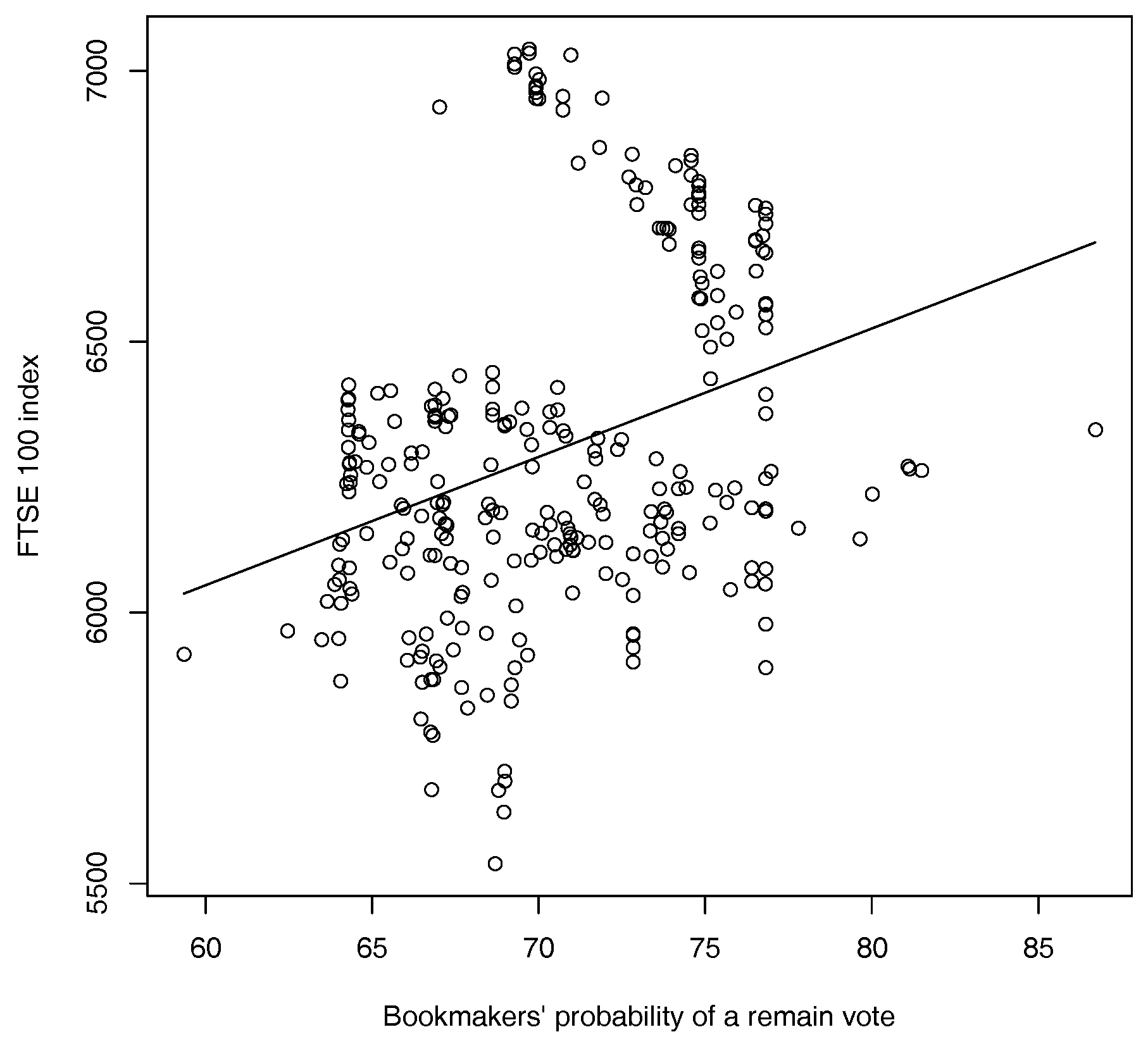
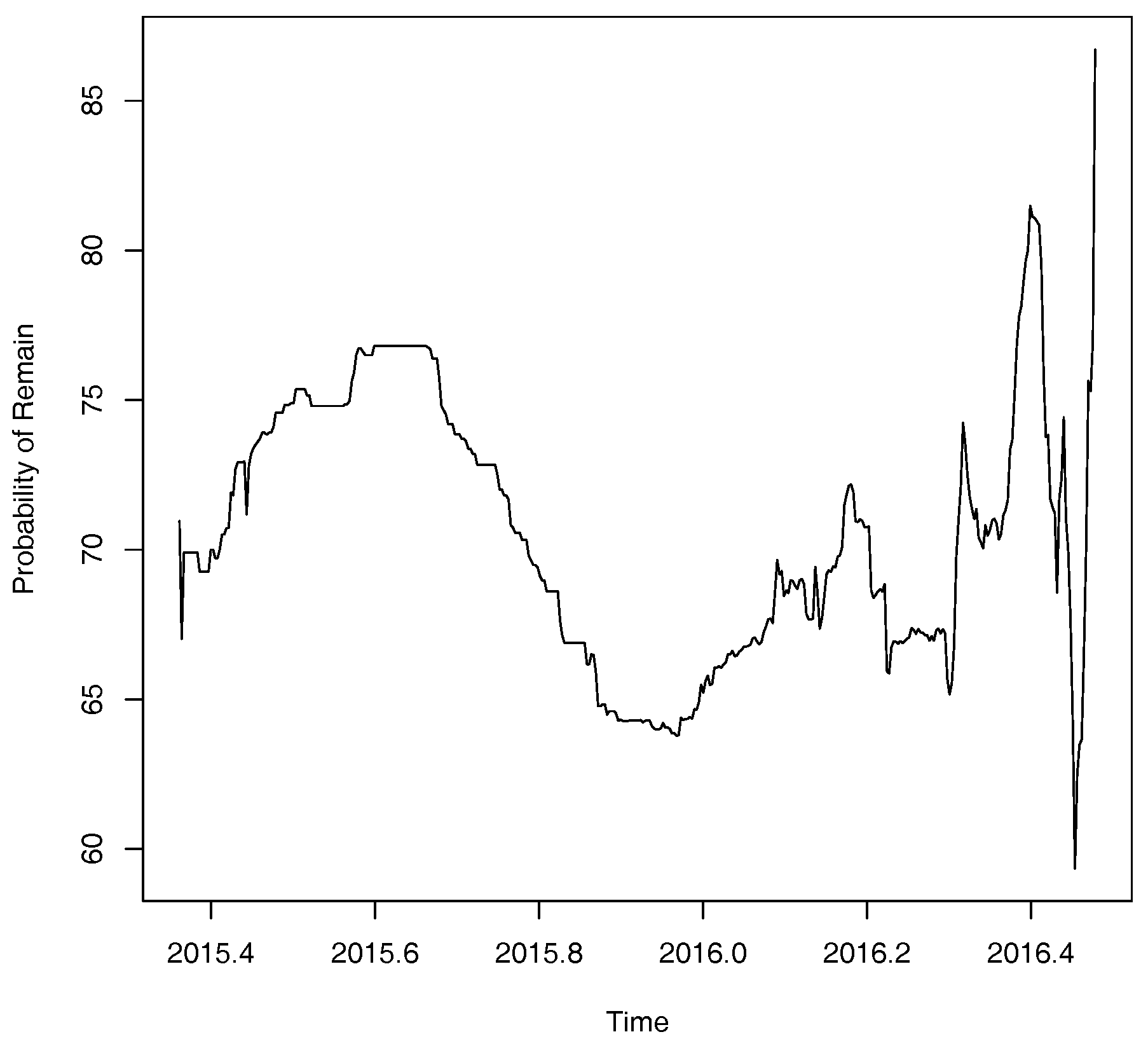
We obtain betting odds from 28 of the UK’s major bookmakers using data obtained from the website www.oddschecker.co.uk. Following Spence (2016) the odds are converted into implied probabilities using basic normalisation (Štrumbelj 2014). These probabilities are then averaged out across the 28 major bookmakers listed to obtain an overall estimate of the probability of a vote in favour of Bremain. A plot of the probability for a vote in favour of remain obtained from bookmakers’ odds is shown below in Figure 2. Though some apparently cyclical behaviour is apparent much more noteworthy is the fact that these probabilities of a remain vote seem to be much higher than might be anticipated on the basis of the polling data in Figure 1. In contrast, it seems that bookmakers’ odds are more closely associated with the price of FTSE 100 stock index with fluctuations in the bookmakers’ estimated probability of a remain vote accounting for over 10% of the variation in the price of the FTSE 100 stock index over the period in question (see Figure 3).
Bookmakers’ odds paint a very different picture of Brexit than do opinion polls. No evidence of a bubble is found (, ). It seems that the competitive payoff structure in betting markets (or even the very existence of such markets) may preclude the formation of bubbles (see, e.g., Vaughan Williams and Reade 2016). Regression results shown below in Table 2 are suggestive of a possible boomakers’ blind spot: their odds do not seem to have been adequately updated in the light of closeness of the final vote that opinion polls suggest. Note that this observation contradicts one of the key assumptions in the theoretical modelling of voting behaviour in Kou and Sobel (2004). Further, this also may be linked to the so-called bias blind spot which is the cognitive bias of recognising bias in the judgement of others whilst failing to see the impact of biases upon one’s own judgement (see, e.g., Pronin et al. 2002). These results also reflect mixed findings in the literature when bookmakers’ odds and opinion polls have previously been used to make political predictions (see, e.g., Leigh and Wolfers 2006; Vaughan Williams and Reade 2016) amidst theoretical and practical considerations that may limit the effectiveness of bookmakers’ odds as a forecasting tool (see, e.g., Shin 1993; Štrumbelj 2014).
5. Conclusions and Further Work
The analogy between financial markets and political systems is very rich - with animal spirits, psychology and herding highly prevalent in both systems (see, e.g., Prechter 1999). Amid the on-going challenge of political prediction (see, e.g., Fisher and Lewis-Beck 2016) referendum polling is known to be highly volatile as the participants lack the tribal loyalties associated with regular elections (Tarran 2016). Here, we make an explicit quantitative link between financial bubbles and political votes. In so doing we find that opinion polls systematically over-price the probability of a remain vote in the EU referendum. Correcting for this bias our model predicts a narrow vote for Brexit by a margin of 50.6–49.4%.
Though imperfect as a forecasting tool their competitive payoff structure may preclude the existence of bubbles in betting markets (Vaughan Williams and Reade 2016). Thus, we find no evidence of a bubble in the betting odds investigated here. However, analysis of the data reveals a bookmakers’ blind spot—with the quoted odds seemingly impervious to polling that indicated a close result (data that nonetheless under-estimated the probability of a vote for Brexit).
The advantages of our approach include theoretical elegance, relative simplicity and ease of use in applications coupled with an ability to account for the irregularly spaced time series commonly found in polling data. Additional work will look at other political applications. These, and related, political prediction problems remain a subject of key academic interest (see, e.g., Fisher 2016; Fisher and Lewis-Beck 2016). Indications are that our model also gives a very reasonable prediction for the 2014 Scottish Independence Referendum (see the Appendix A). Further, the parallels between the EU referendum and the recent US presidential election appear striking. Our model may be used to make more precise forecasts whenever there is a suspicion of systematic bias in polling results due to the Bradley effect and related phenomena. For the EU Referendum it is relatively easy to see how a Bradley effect over-estimates the probability of a remain vote. However, in other settings it may be harder to determine in advance the way in which such a Bradley effect may materialise and this may be a limitation in future work. Future work will analyse spread betting markets where the information processing and underlying market mechanisms are undeniably more complex. Future work will also examine the application of related methods to the issues of risk, failure and lack of foresight in other complex social systems—see, e.g., Chernov and Sornette (2016).
Acknowledgments
The authors would like to acknowledge constructive comments from three anonymous referees as well as interesting discussions with Ibrahim Al-Ghraify and Jean-Philippe Serbera. The usual disclaimer applies.
Author Contributions
Both authors jointly came up with the basic ideas under-pinning the paper. John Fry composed the model, performed the data analysis and wrote the manuscript. Andrew Brint provided the data and contributed further ideas and technical support to all aspects of the paper.
Conflicts of Interest
The authors report no conflict of interest.
Appendix A. The 2014 Scottish Independence Referendum
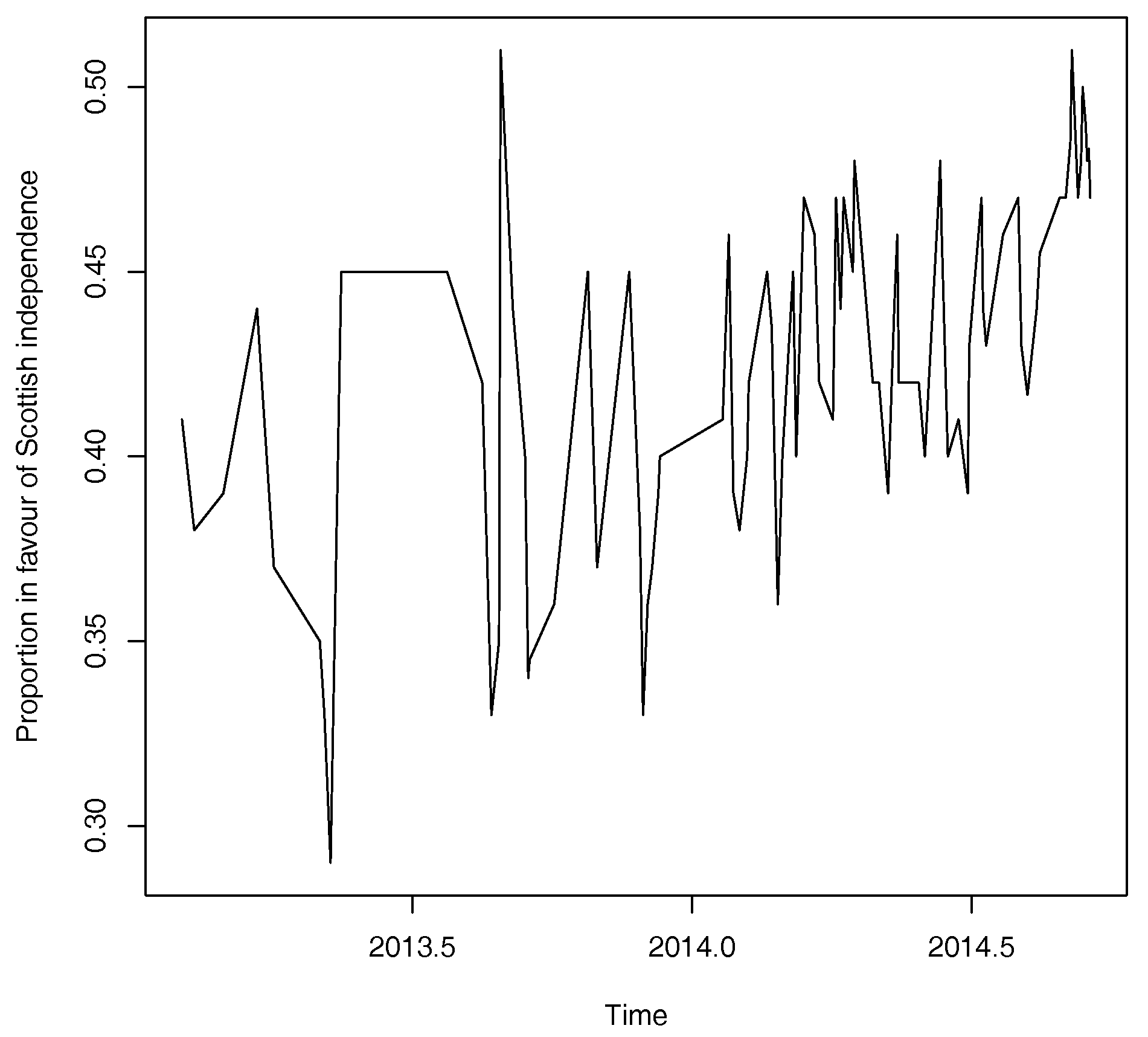
In this section we consider an additional empirical application to the 2014 Scottish Independence Referendum. Polling data are obtained from the non-partisan website whatscotlandthings.org. A plot of the proportion in favour of Scottish independence (“don’t know” responses removed) is shown below in Figure A1 and shows a dramatic increase over time. It is therefore natural to ask if this growth over time constitutes a speculative bubble.
Figure A1.
Proportion in favour of Scottish Independence: results of opinion polls with “don’t know” responses removed. Data from 1 February 2013–17 September 2014 (Source: http://whatscotlandthinks.org.)
Figure A1.
Proportion in favour of Scottish Independence: results of opinion polls with “don’t know” responses removed. Data from 1 February 2013–17 September 2014 (Source: http://whatscotlandthinks.org.)

A likelihood ratio test gives a clear indication of the presence of a speculative bubble: , . Equation (18) gives a value of 0.1309 with an associated 95% Confidence Interval of (0.0624, 0.1994). This suggests that for these opinion polls the odds ratio for the proportion voting for Scottish Independence is about 13% over-valued. Given this apparent over-pricing, together with the dramatic increase over time, a more reasonable estimate for the proportion who will vote for Scottish Independence can be obtained by setting,
where denotes the day before the Scottish Referendum vote takes place. A 95% Confidence Interval corresponding to Equation (A1) is given by (0.4152, 0.4540). A corresponding simple normal approximation suggests a vote in favour of Scottish Independence is highly unlikely. These predictions match well with a final vote against Scottish independence in the referendum by a margin of 55.3–44.7%. In summary, the suggestion is that in the 2014 Scottish Independence Referendum opinion polls contain a speculative bubble component that exaggerates the likelihood of a vote in favour of independence.
References
- Alesina, Alberto, and Nouriel Roubini. 1992. Political cycles in OECD economies. The Review of Economic Studies 59: 663–88. [Google Scholar] [CrossRef] [Green Version]
- Berg, Joyce E., Forrest D. Nelson, and Thomas A. Rietz. 2008. Prediction market accuracy in the long run. International Journal of Forecasting 24: 285–300. [Google Scholar] [CrossRef]
- Bingham, Nicholas H., and John M. Fry. 2010. Regression: Linear Models in Stattics. London, Dordtrecht, Heidelberg, New York: Springer. [Google Scholar]
- Blanchard, Olivier J., and Mark W. Watson. 1982. Bubbles, rational expectations and financial markets. In Crises in the Economic and Financial Structure. Edited by P. Wachtel. Lexington: D. C. Heathand Company, pp. 295–316. [Google Scholar]
- Cheah, Eng-Tuck, and John Fry. 2015. Speculative bubbles in Bitcoin markets? An empirical investigation into the fundamental value of Bitcoin. Economics Letters 130: 32–36. [Google Scholar] [CrossRef]
- Chernov, Dmitry, and Didier Sornette. 2016. MAn-Made Catastrophes and Risk Information Concealment. Heidelberg, New York, Dordtrecht, London: Springer. [Google Scholar]
- Clark, Iain J., and Saeed Amen. 2017. Implied distributions from GBPUSD risk-reversals and implication for Brexit scenarios. Risks 5: 35. [Google Scholar] [CrossRef]
- Diba, Behzad T., and Herschel I. Grossman. 1988. Explosive rational bubbles in stock prices? The American Economic Review 78: 520–30. [Google Scholar]
- Erikson, Robert S., and Christopher Wlezien. 2008. Are political markets really superior to polls as election predictors? Public Opinion Quarterly 72: 190–215. [Google Scholar] [CrossRef]
- Erikson, Robert S., and Christopher Wlezien. 2012. Markets vs. polls as election predictors: An historical assessment. Electoral Studies 31: 532–39. [Google Scholar] [CrossRef]
- Evans, George W. 1991. Pitfalls in testing for explosive bubbles in asset prices. The American Economic Review 81: 922–30. [Google Scholar]
- Fama, Eugene F., and Kenneth R. French. 1988. Permanent and transitory components of stock prices. Journal of Political Economy 96: 246–73. [Google Scholar] [CrossRef]
- Fisher, Stephen D. 2016. Putting it all together and forecasting who governs: The 2015 British general election. Electoral Studies 41: 234–38. [Google Scholar] [CrossRef]
- Fisher, Stephen D., and Michael S. Lewis-Beck. 2016. Forecasting the 2015 British general election: The 1992 debacle all over again? Electoral Studies 41: 225–29. [Google Scholar] [CrossRef]
- Ford, Robert, Will Jennings, Mark Pickup, and Christopher Wleizen. 2016. From polls to votes to seats: Forecasting the 2015 British general election. Electoral Studies 41: 244–49. [Google Scholar] [CrossRef]
- Fry, John. 2012. Exogenous and endogenous crashes as phase transitions in complex financial systems. The European Physical Journal B 85: 405. [Google Scholar] [CrossRef] [Green Version]
- Fry, John. 2015. Stochastic modelling for financial bubbles and policy. Cogent Economics and Finance 3: 1002152. [Google Scholar] [CrossRef]
- Fry, John, and Eng-Tuck Cheah. 2016. Negative bubbles and shocks in cryptocurrency markets. International Review of Financial Analysis 47: 343–52. [Google Scholar] [CrossRef]
- Gandar, John, Richard Zuber, Thomas O’Brien, and Ben Russo. 1988. Testing rationality in the point spread betting market. The Journal of Finance 43: 995–1008. [Google Scholar] [CrossRef]
- Gürkaynak, Refet S. 2008. Econometric tests of asset price bubbles: Taking stock. Journal of Economic Surveys 22: 166–86. [Google Scholar] [CrossRef]
- Harras, Georges, and Didier Sornette. 2011. How to grow a bubble: A model of myopic adapting agents. Journal of Economic Behavior and Organization 80: 137–52. [Google Scholar] [CrossRef]
- Hendershott, Patric H., Robert J. Hendershott, and Charles R.W. Ward. 2003. Corporate equity and commercial property market “bubbles”. Urban Studies 40: 993–1003. [Google Scholar] [CrossRef]
- Herron, Michael C., James Lavin, Donald Cram, and Jay Silver. 1999. Measurement of political effects in the United States economy: A study of the 1992 presidential election. Economics and Politics 11: 51–80. [Google Scholar] [CrossRef]
- Hoffmann, Mathias, Michael U. Krause, and Thomas Laubach. 2012. Trend growth expectations and U.S. house prices before and after the crisis. Journal of Economic Behavior and Organization 83: 394–409. [Google Scholar] [CrossRef]
- Hott, Christian, and Pierre Monnin. 2008. Fundamental real estate prices: An empirical estimation with international data. The Journal of Real Estate Finance and Economics 36: 427–50. [Google Scholar] [CrossRef]
- Hüsler, Andreas, Didier Sornette, and Cars H. Hommes. 2013. Super-exponential bubbles in lab experiemnts: Evidence for anchoring over-optimistic expectations on price. Journal of Economic Behavior and Organization 92: 304–16. [Google Scholar] [CrossRef]
- Hyman, Herbert. 1944. Do they tell the truth? The Public Opinion Quarterly 8: 557–59. [Google Scholar] [CrossRef]
- Johansen, Anders, Olivier Ledoit, and Didier Sornette. 2000. Crashes as critical points. International Journal of Theoretical and Applied Finance 3: 219–55. [Google Scholar] [CrossRef]
- Johnson, Dominic. 2004. Overconfidence and War: The Havoc and Glory of Positive Illusions. Cambridge: Harvard University Press. [Google Scholar]
- Kindelberger, Charles P., and Robert Z. Aliber. 2005. Manias, Panics and Crashes: A History of Financial Crises, 5th ed. Hoboken: Wiley. [Google Scholar]
- Kou, Steven G., and Michael E. Sobel. 2004. Forecasting the vote: A theoretical comparison of election markets and public opinion polls. Political Analysis 12: 277–95. [Google Scholar] [CrossRef]
- Lad, Frank. 1996. Operational, Subjective Statistical Methods: A Mathematical, Philosophical and Historical Introduction. New York: Wiley. [Google Scholar]
- Leigh, Andrew, and Justin Wolfers. 2006. Competing approaches to forecasting elections: economic models, opinion polling and prediction markets. Economic Record 82: 325–40. [Google Scholar] [CrossRef]
- Lewis-Beck, Michael S., Richard Nadeau, and Eric Bélanger. 2016. The British general election: Synthetic forecasts. Electoral Studies 41: 264–68. [Google Scholar] [CrossRef]
- Little, Roderick J.A. 1988. Missing-data adjustments in large surveys. Journal of Business and Economic Statistics 6: 287–301. [Google Scholar] [CrossRef]
- Maillart, T., D. Sornette, S. Frei, T. Duebendorfer, and A. Saichev. 2011. Quantification of deviations from rationality with heavy tails in human dynamics. Physical Review E 83: 056101. [Google Scholar] [CrossRef] [PubMed]
- Malmendier, Ulrike, and Geoffrey Tate. 2005. CEO overconfidence and corporate investment. The Journal of Finance 60: 2661–700. [Google Scholar] [CrossRef]
- Moore, Don A., and Paul J. Healy. 2008. The trouble with overconfidence. Psychological Review 208: 502–17. [Google Scholar] [CrossRef] [PubMed]
- Murr, Andreas E. 2016. The wisdom of crowds: What do citizens forecast for the 2015 British general election? Electoral Studies 41: 283–88. [Google Scholar] [CrossRef]
- Oehler, Andreas, Matthias Horn, and Stefan Wendt. 2017. Brexit: Short-term stock price effects and the impact of firm-level internationalization. Finance Research Letters 22: 175–81. [Google Scholar] [CrossRef]
- Payne, J. Gregory. 2010. The Bradley Effect:mediated reality of race and politics in the 2008 US presidential election. American Behavioral Scientist 54: 417–35. [Google Scholar] [CrossRef]
- Prechter, Robert Rougelot, Jr. 1999. The Wave Principle of Human Behaviour and the New Science of Socionomics. Gainesville: New Classics Library. [Google Scholar]
- Prechter, Robert R., Jr., Deepak Goel, Wayne D. Parker, and Matthew Lampert. 2012. Social mood, stock market performance, and US presidential elections: A socionomic perspective on voting results. SAGE Open 2: 2158244012459194. [Google Scholar] [CrossRef]
- Pronin, Emily, Daniel Y. Lin, and Lee Ross. 2002. The bias blind spot: perceptions of bias in self versus others. Personality and Social Psychology Bulletin 28: 369–81. [Google Scholar] [CrossRef]
- Rhode, Paul W., and Koleman S. Strumpf. 2004. Historical presidential betting markets. The Journal of Economic Perspectives 18: 127–42. [Google Scholar] [CrossRef]
- Rogoff, Kenneth S. 1990. Equilibrium political business cycles. The American Economic Review 80: 21–36. [Google Scholar]
- Rothschild, David. 2009. Forecasting elections: comparing prediction markets, polls and their biases. Public Opinion Quarterly 73: 895–916. [Google Scholar] [CrossRef]
- Rubin, Donald B., Hal S. Stern, and Vasja Vehovar. 1995. Handling “don’t know” survey responses: The case of the Slovenian plebiscite. Journal of the American Statistical Association 90: 822–28. [Google Scholar] [CrossRef]
- Shiller, Robert J. 2005. Irrational Exuberance, 2nd ed. Princeton: Princeton University Press. [Google Scholar]
- Shin, Hyun Song. 1993. Measuring the incidence of insider trading in a market for state-contingent claims. The Economic Journal 103: 1141–53. [Google Scholar] [CrossRef]
- Sornette, D. 2003. Why Stock Markets Crash: Critical Events in Complex Financial Systems. Princeton: Princeton University Press. [Google Scholar]
- Sornette, Didier. 2006. Critical Phenomena in Natural Sciences: Chaos, Fractals, Selforganization and Disorder: Concepts and Tools, 2nd ed. Berlin, Heidelberg: Springer.
- Spence, Peter. 2016. Will the UK Leave the EU? Keeping Track of the Polls, Bookmaker Odds, and the Financial Markets. The Daily Telegraph. June 20. Available online: http://www.telegraph.co.uk/business/2016/02/22/will-the-uk-leave-the-eu-how-to-track-the-odds-of-a-brexit/ (accessed on 17 July 2017).
- Spence, Peter, and Tim Wallace. 2016. City Bets on Pound to Suffer Bigger Plunge Than ‘Black Wednesday’ After Brexit Vote. The Daily Telegraph. June 18. Available online: http://www.telegraph.co.uk/business/2016/06/18/city-bets-on-pound-to-suffer-bigger-plunge-than-black-wednesday (accessed on 17 July 2017).
- Štrumbelj, Erik. 2014. On determining probability forecasts from betting odds. International Journal of Forecasting 30: 934–43. [Google Scholar] [CrossRef]
- Summers, Lawrence H. 1986. Does the stock market rationally reflect fundamental values? The Journal of Finance 41: 591–603. [Google Scholar] [CrossRef]
- Tarran, Brian. 2016. The economy: A Brexit vote winner? Significance 13: 6–7. [Google Scholar] [CrossRef]
- Vaughan Williams, L. 1999. Information efficiency in betting markets: A survey. Bulletin of Economic Research 51: 1–39. [Google Scholar] [CrossRef]
- Vaughan Williams, L., and J. James Reade. 2016. Forecasting elections. Journal of Forecasting 35: 308–28. [Google Scholar] [CrossRef]
- Whiteley, Paul. 2016. Why do voters lie to the pollsters? Political Insight 7: 16–19. [Google Scholar] [CrossRef]
- Yan, Wanfeng, Ryan Woodard, and Didier Sornette. 2012. Diagnosis and prediction of rebounds in financial markets. Physica A: Statistical Mechanics and its Applications 391: 1361–80. [Google Scholar] [CrossRef]
- Zeira, Joseph. 1997. Informational overshooting, booms and crashes. Journal of Monetary Economics 43: 237–57. [Google Scholar] [CrossRef]
- Zhou, Wei-Xing, and Didier Sornette. 2006. Is there a real-estate bubble in the US? Physica A: Statistical Mechanics and Its Applications 361: 297–308. [Google Scholar] [CrossRef]
| 1 | By over-confident we mean over-precise in their estimates of the underlying risks involved (see Section 3). |
| 2 | The average number of “don’t know” responses in the opinion polls studied here is 15% (standard deviation 0.35%). Omitting “don’t know” responses follows the standard way in which opinion poll data has been used to make political forecasts in the literature (see, e.g., Leigh and Wolfers 2006). Further, the closeness of the final vote coupled with empirical evidence from general survey modelling (Little 1988) and other political modelling work (Rubin et al. 1995) suggests that this approach should lead to reasonable results in practice. Non-ignorable missing data models for political polls have been considered in related problems (Rubin et al. 1995). However, this would require additional modelling assumptions that in practice would be difficult justify and would be unlikely to lead to significant improvements (see, e.g., Rubin et al. 1995). |
Figure 1.
Proportion in favour of Bremain: results of opinion polls with “don’t know” responses removed together with the fit of a simple linear time trend model. (Source: National Centre for Social Research.)
Figure 1.
Proportion in favour of Bremain: results of opinion polls with “don’t know” responses removed together with the fit of a simple linear time trend model. (Source: National Centre for Social Research.)
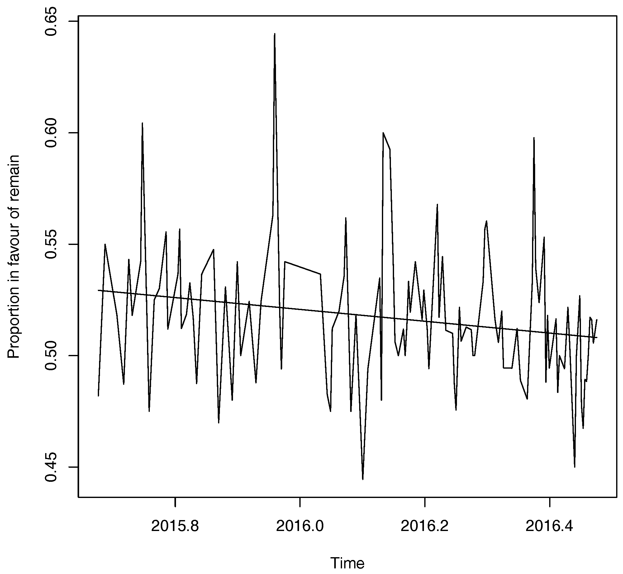
Figure 2.
Plot of bookmakers’ implied probability of a remain vote in the EU referendum from 11 May 2015–23 June 2016. (Source: www.oddschecker.com.)
Figure 2.
Plot of bookmakers’ implied probability of a remain vote in the EU referendum from 11 May 2015–23 June 2016. (Source: www.oddschecker.com.)

Figure 3.
Plot of FTSE 100 stock index against bookmakers’ implied probability of a remain vote in the EU referendum from 11 May 2015–23 June 2016 together with a fitted regression line (, ). (Sources: www.oddschecker.com and www.google.com/finance.)
Figure 3.
Plot of FTSE 100 stock index against bookmakers’ implied probability of a remain vote in the EU referendum from 11 May 2015–23 June 2016 together with a fitted regression line (, ). (Sources: www.oddschecker.com and www.google.com/finance.)

Table 1.
Likelihood ratio test for the presence or absence of a speculative bubble: rolling window estimates.
Table 1.
Likelihood ratio test for the presence or absence of a speculative bubble: rolling window estimates.
| Dates | p-Value | |
|---|---|---|
| September 2015–January 2016 | 7.2002 | 0.0072 |
| September 2015–Feburary 2016 | 14.0192 | 0.0002 |
| September 2015–March 2016 | 12.0572 | 0.0005 |
| September 2015–April 2016 | 9.4774 | 0.0021 |
| September 2015–May 2016 | 20.4255 | 0.0000 |
| September 2015–June 2016 | 13.5763 | 0.0002 |
Table 2.
Regression of bookmaker probability of remain against opinion poll proportion and at times t and respectively.
Table 2.
Regression of bookmaker probability of remain against opinion poll proportion and at times t and respectively.
| Parameter | Estimate (t-Value) | Estimate (t-Value) |
|---|---|---|
| Constant | 69.8372 *** | 70.277 *** |
| (10.885) | (11.028) | |
| −0.8938 | ||
| (−0.067) | ||
| 13.169 | ||
| (−0.147) |
© 2017 by the authors. Licensee MDPI, Basel, Switzerland. This article is an open access article distributed under the terms and conditions of the Creative Commons Attribution (CC BY) license (http://creativecommons.org/licenses/by/4.0/).
Share and Cite
MDPI and ACS Style
Fry, J.; Brint, A. Bubbles, Blind-Spots and Brexit. Risks 2017, 5, 37. https://doi.org/10.3390/risks5030037
AMA Style
Fry J, Brint A. Bubbles, Blind-Spots and Brexit. Risks. 2017; 5(3):37. https://doi.org/10.3390/risks5030037
Chicago/Turabian StyleFry, John, and Andrew Brint. 2017. "Bubbles, Blind-Spots and Brexit" Risks 5, no. 3: 37. https://doi.org/10.3390/risks5030037
Note that from the first issue of 2016, this journal uses article numbers instead of page numbers. See further details here.