
Stress Testing German Industry Sectors: Results from a Vine Copula Based Quantile Regression

1
Lehrstuhl für Statistik und Ökonometrie, Universität Erlangen-Nürnberg, Lange Gasse 20, 90403 Nürnberg, Germany
2
Zentrum Mathematik, Technische Universität München, Boltzmanstraße 3, 85748 Garching, Germany
*
Author to whom correspondence should be addressed.
Risks 2017, 5(3), 38; https://doi.org/10.3390/risks5030038
Submission received: 14 April 2017
/
Revised: 12 July 2017
/
Accepted: 13 July 2017
/
Published: 19 July 2017
(This article belongs to the Special Issue Quantile Regression for Risk Assessment)
Abstract
:Measuring interdependence between probabilities of default (PDs) in different industry sectors of an economy plays a crucial role in financial stress testing. Thereby, regression approaches may be employed to model the impact of stressed industry sectors as covariates on other response sectors. We identify vine copula based quantile regression as an eligible tool for conducting such stress tests as this method has good robustness properties, takes into account potential nonlinearities of conditional quantile functions and ensures that no quantile crossing effects occur. We illustrate its performance by a data set of sector specific PDs for the German economy. Empirical results are provided for a rough and a fine-grained industry sector classification scheme. Amongst others, we confirm that a stressed automobile industry has a severe impact on the German economy as a whole at different quantile levels whereas, e.g., for a stressed financial sector the impact is rather moderate. Moreover, the vine copula based quantile regression approach is benchmarked against both classical linear quantile regression and expectile regression in order to illustrate its methodological effectiveness in the scenarios evaluated.
1. Motivation
Generally speaking, stress testing identifies potential vulnerabilities of financial institutions under hypothetical or historical scenarios. Financial institutions typically perform stress tests to assess possible short-term losses resulting from various types of risk (e.g., credit risk, market risk, operational risk). The history of stress tests in the banking industry dates back to the early 1990s, where large banks started to initiate internal stress exercises. In 1996, the Basel Capital Accord was amended which requires banks to conduct stress tests and determine their ability to respond to market events. However, up until 2007, stress tests were typically performed only by the banks themselves, for internal self-assessment. Beginning in 2007, regulatory institutions became interested in conducting their own stress tests to ensure the effective operation of financial institutions. Since then, stress tests have been routinely performed by financial regulators in different countries or regions, to ensure that the banks under their authority are engaging in practices likely to avoid negative outcomes. Recently, the European Banking Authority (EBA) published the results of the 2016 EU-wide stress test of 51 banks. The aim of this stress test was to assess the resilience of EU banks to adverse economic developments. Similarly, the Federal Reserve Board currently published the scenarios to be used by banks and supervisors for the 2017 Comprehensive Capital Analysis and Review (CCAR) and Dodd-Frank Act stress test exercises. The focus within this work is on stress testing credit risk and losses associated therewith. Typically, the loan portfolios of the banking sector consist of financial obligations to counterparties from different business lines. Hence, the key source of credit risk in that portfolio is that a counterparty may default, which would result in losses for the bank. Secondly, one has to be aware of (industry/country) sector risk which means that multiple clients within an industry sector default because of structural weaknesses within this sector. Finally, even counterparties from different sectors may tend to default together in economic downturns, e.g., if only one (industry/country) sector enters a crisis and these sectors are highly dependent with the other. In all cases, the primary interest lies in the explanation (in a first step) and the initiation of stress (in a second step) of the counterparties’ probability of default (PD).
In this context, quantile regression (QR) is an increasingly important empirical tool in economics and other sciences for analyzing the impact a set of regressors (e.g., macro-economic variables) has on the conditional distribution of an outcome (here: PD). In the context of stress testing, the focus is on rare events arising from the tails of the distribution, which motivates the application of so-called extremal QR, or QR applied to the tails, (see, e.g., Chernozhukov (2005) of Chernozhukov et al. (2017)). The quantile regression method is used to estimate parameters in accordance with the distribution of a dependent variable. One could use high quantile values of these distributions such as the 95th percentile value for a period in which large stresses occur. For a period in which no stresses are exerted on the economy, normal parameters estimated by the least square method might come to application.
Extremal QR was applied by Koenker and Xiao (2002), Schechtman and Gaglianone (2012), Covas et al. (2014) and Ong (2014) within a macro-credit risk link context, i.e., connecting PDs and macro-economic variables. In contrast to these studies, we apply extremal QR to investigate how crises (in the sense of higher PDs) in industry sectors are connected to other industry sectors. Above that, we circumvent the disadvantages of classical QR, namely the occurrence of so-called quantile-crossings and apply D-vine copula based quantile regression as recently advocated by Kraus and Czado (2017a), instead. Against this background, the outline of this work is as follows: Section 2 briefly reviews D-vines and D-vine copula based regression. Section 3 is dedicated to the empirical study which relies on (averaged) default probabilities of 9 different German industry sectors and selected subgroups. After a brief description of the underlying data set, the data transformation to the copula scale and the resulting data structure is discussed. A D-vine based copula regression is performed and highlights are presented. Finally, we illustrate its superiority to alternative approaches such as traditional quantile regression and expectile regression. Section 4 concludes.
2. A Short Review on D-Vines and D-Vine Copula Based Quantile Regression
Copulas are important and useful tools to model the dependence between financial variables. They allow separate considerations of marginal distributions and dependencies due to Sklar’s Theorem (Sklar 1959), which states that the joint distribution F of a continuous random vector can be expressed in terms of its marginal distributions , , and its unique copula through the relationship
This formula facilitates flexible modeling of multivariate distributions, since the marginals and the dependence function C can be modeled separately. Another consequence of Sklar’s Theorem is that, as long as the interest lies in the dependence between random variables, one can consider the probability integral transformed random variables , , which are uniformly distributed. We say that these variables and their realizations are on the copula scale. Thorough introductions to copulas are given in Joe (1997) and Nelsen (2006). The reader shall notice that in this manuscript only continuous random variables are discussed. Nevertheless, extensions for discrete variables are available.
In high dimensions many parametric copula models lack flexibility. For example, the exchangeable Archimedean copulas only have one or two dependence parameters (see, e.g., McNeil and Nešlehová 2009) and elliptical copulas always exhibit symmetric dependencies in the tails (see, e.g., Frahm et al. 2003). Vine copulas overcome these shortcomings by breaking down the modeling of a multivariate copula to the fitting of several bivariate copulas (Aas et al. 2009; Bedford and Cooke 2002; Fischer et al. 2009), e.g., in three dimensions a vine copula density decomposition is given by
where the three pair-copulas , and can be modeled separately, each with its own parametric copula family and dependence parameter(s). The arguments of the conditional copula , namely and , are obtained by taking derivatives, i.e., , (see Joe 1997). Note that choosing only bivariate Gaussian copulas in the decomposition always results in a multivariate Gaussian copula.
To conduct statistical inference it is usually assumed that the conditional copula does not depend on , i.e., . This so-called simplifying assumption has been inspected by many researchers (see e.g., Killiches et al. 2017; Spanhel and Kurz 2015; Stöber et al. 2013). While there exist cases where it is a model restriction, empirical studies show that the assumption is not a severe restriction for financial data sets, see Kraus and Czado (2017b) or Hobæk Haff et al. (2010). However, the implications of the simplifying assumption on the tails of a distribution have not been explicitly studied and therefore are still subject to further research.
A special subclass of vine copulas that we will use to model the dependence between default probabilities of German industry sectors are D-vine copulas. The decomposition of a d-dimensional simplified D-vine copula density can be seen as a generalization of Equation (1) and is given by
Thus, modeling a d-dimensional D-vine copula consists of fitting bivariate parametric copulas, so-called pair-copulas. The arguments of the pair-copulas are obtained from a recursive formula given in Joe (1997) using the specified pair-copulas.
For the purpose of stress testing we are interested in estimating conditional quantiles of a response variable conditioned on predictor variables :
The general process to obtain predictions of such conditional quantiles given covariates by modeling the complete dependence structure between all variables and V shall in the following be referred to as copula based quantile regression. Given a fully specified D-vine copula with response V as first variable, the conditional copula quantile function can be analytically expressed only using the pair-copulas of the D-vine (see Kraus and Czado 2017a). This is not possible for an arbitrary regular vine, which is why we use D-vine copulas.
The only question remaining is how to fit the D-vine to given copula data (i.e., specifying the order of the D-vine and the pair-copulas), such that predictions of its conditional quantile functions are optimal. Kraus and Czado (2017a) propose an algorithm, which sequentially adds covariates to the D-vine that improve the model fit (measured in terms of the log-likelihood of the conditional density ) the most. Starting with an empty model, in the first step each of the d covariates is separately added to the model and a maximum likelihood estimate for the pair-copula is fitted. Then, the covariate resulting in the model with the highest conditional log-likelihood is chosen as the first variable in the D-vine. In the next step, each of the remaining covariates is again separately added to the current model and we choose the one with the best fit with regard to the conditional log-likelihood. This is done until none of the remaining covariates is able to improve the model fit. Thus, the algorithm facilitates an automatic forward covariate selection. The authors further demonstrate that D-vine copula based quantile regression outperforms traditional quantile regression methods established in the literature regarding prediction accuracy.
3. Data Description and Empirical Results
3.1. Original Data Set
For parameter estimation, a data pool with German exchange traded corporates is used. Based on a standard Merton model (see Merton 1974), the original time series consist of 112 one-year PDs between May 2007 and September 2016. The PDs which are available monthly over the time horizon and on company level are averaged on sector level, using a market-based classification scheme, similar to the GICS and ICB systems with 9 industry sectors (Basic Materials, Communications, Cyclical Consumer Goods & Services, Non-cyclical Consumer Goods & Services, Energy, Financials, Industrials, Technology, Utilities) and several industry groups for a finer classification scheme. More precisely, PD’s within a Merton setting estimate the probability that a firm will default over a specified period of time (here: one year). As usually, “default” is defined as failure to make scheduled principal or interest payments. In the Merton setting, a firm defaults when the market value of its assets falls below its liabilities payable. Hence, the relevant drivers are the current market value of the firm, the level of the firm’s obligations and the vulnerability/sensitivity of the market value to large changes. Exemplarily, Figure 1 illustrates the “PD history” for Financials with significant peaks caused by the last financial crisis from 2007 to 2008.
3.2. Time Dependencies and Transformation to Copula Scale
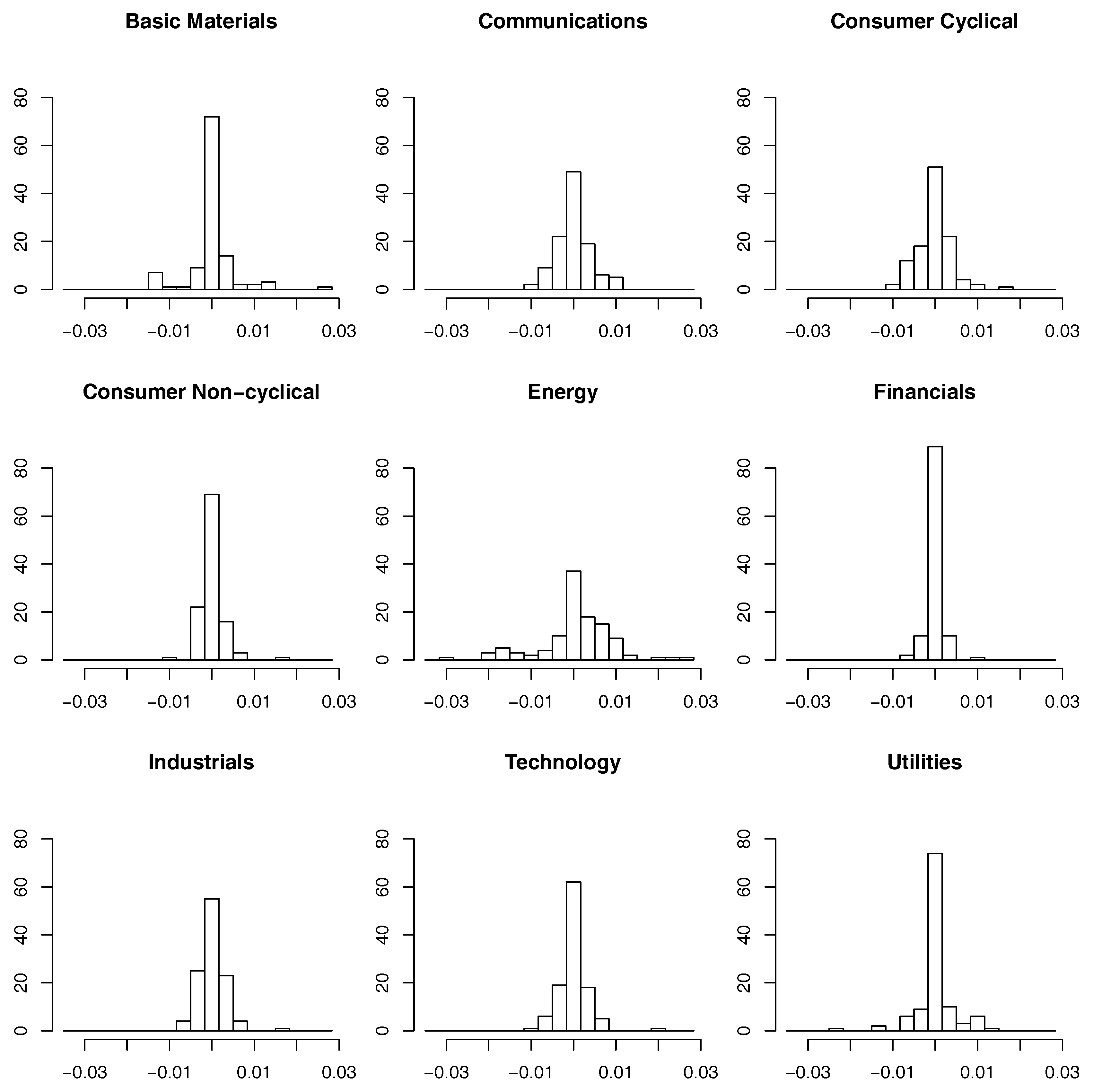
We consider the monthly differences of the aggregated sector PDs on a rough as well as on a more detailed level. Histograms of the differenced data on the rough level are displayed in Figure 2. The differenced data series are stationary and do not exhibit any autocorrelation or volatility clustering. Therefore, no ARMA-GARCH models are necessary to account for time dependencies.
Next, we transform the differenced data to the copula scale by applying the probability integral transform using the kernel density estimators as marginal distribution functions (as described in detail in Kraus and Czado 2017a). The corresponding contour plots with standard normal margins and Kendall’s values are displayed in Figure 3. With very homogenous bootstrap standard errors for the individual pairwise industry sector combinations, we derive the average bootstrap standard error as . Thus, empirical Kendall’s tau estimates larger than 0.131 can be seen as significantly different from the independence case in the sense of not being within the bounds of a Wald confidence interval in this case.
The dependencies are weak to medium and mostly positive, at first glance. The Industrials sector seems to have the strongest interdependencies with the other ones. The empirical copula density contours with standard normal margins suggest that the dependencies are quite asymmetric, such that Gaussian copulas or elliptical copulas in general would not provide reasonable fits. Some pairs seem to exhibit tail dependence (e.g., Industrials and Technology). The histograms of the transformed marginals displayed on the diagonal are reasonably flat for a sample of this size.
3.3. Selected Results of the D-Vine Copula Based Quantile Regression
In the following, we will describe the stress scenario which is applied to the data set and how D-vine copula based quantile regression is employed to perform the tests. We present selected results which are on the one hand interesting in the sense of crucial to the German industry or on the other hand show exemplary interpretations of the estimated outcomes.
3.3.1. The Stress Scenario
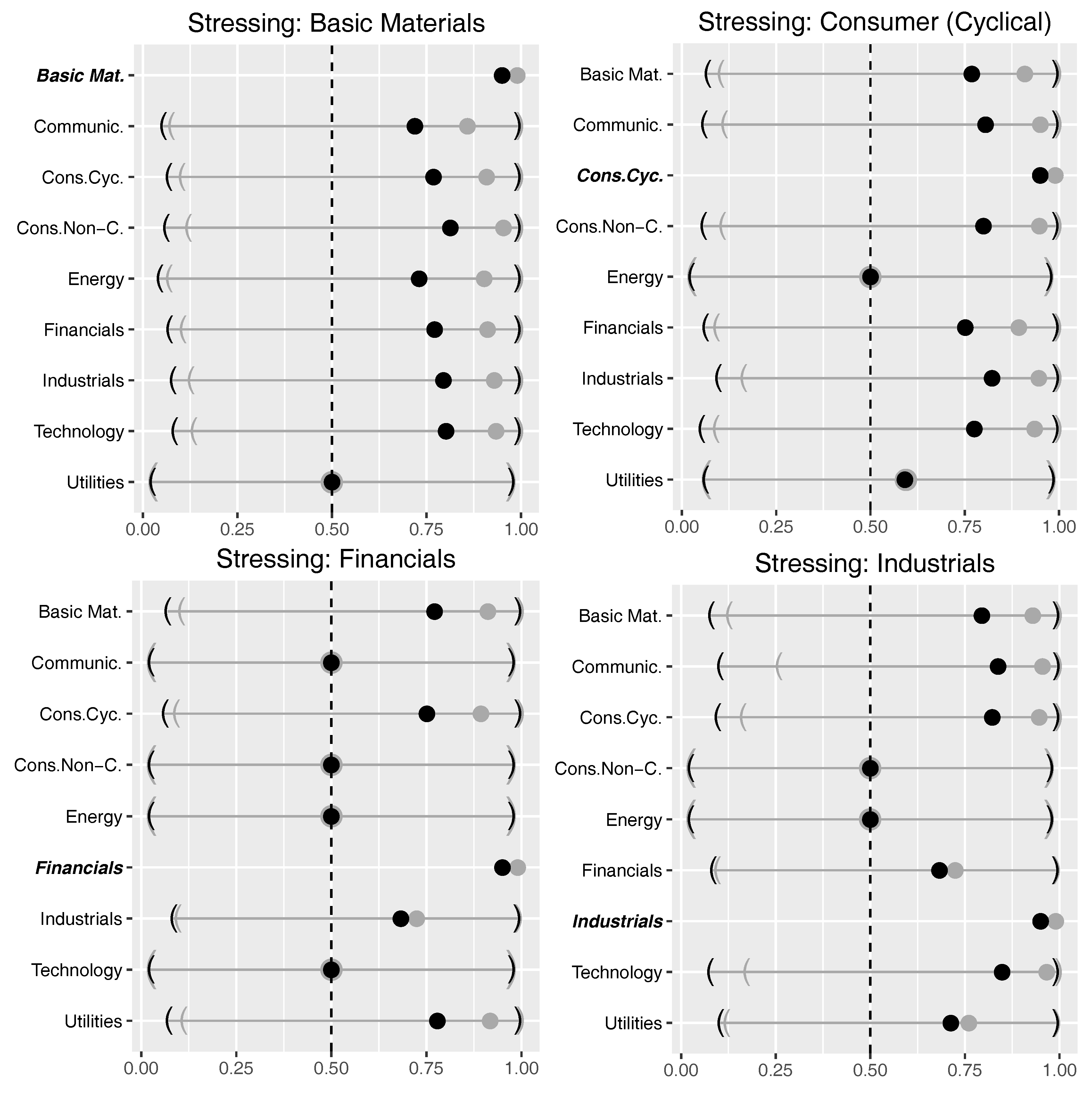
In a nutshell, the stress scenario setup is that we induce stress on a single industry sector and evaluate how this affects the other sectors by employing D-vine copula based quantile regression. Thus, the single stressed industry sector is a covariate in the regression model and all other sectors response variables. This is similar to the stress scenarios described in Kraus and Czado (2017a). The sector variables are evaluated on the copula scale. Thus, large values (i.e., close to 1) of the variables correspond to large differences in the sector PDs. Inducing stress on an industry sector will be treated as setting the value of the respective industry sector covariate to a predetermined quantile level , in our scenario . Thus, we apply what is referred to as extremal QR in the introduction and this yields the intuitive interpretation that the covariate is stressed to or of its potential range exhibited by the data. We use D-vine quantile regression to examine the effect of stressed companies (covariates) on the other companies (responses). Separate models are estimated so that only one sector is stressed at a time and the impact of this scenario on all other sectors evaluated. This impact is quantified by predicted quantiles for the response companies. Note that since we are only considering two-dimensional models in Section 3.3.2, we do not have to make the simplifying assumption here. In our study, we predict the median of the response sectors. Large deviations of the conditional predicted median from the unconditional median of 0.5 imply strong effects of the stress scenario. In the graphics in Figure 4 and Figure 5 the black (and grey) points stand for (and ) conditional median predictions, the brackets for the corresponding confidence intervals and the dashed line at the center for the unconditional median.
3.3.2. Results for Stressing at 95% and 99% on Aggregated Data
At first we present the results on the aggregated data, stressing one sector at stress levels (black) and (gray). For reasons of brevity, our focus lies on the sectors Basic Materials (upper left panel of Figure 4), Cyclical Consumer Goods (upper right panel of Figure 4), Financials (lower left panel of Figure 4) and Industrials (lower right panel of Figure 4).
As expected, the effect on the conditional quantile functions strongly depends on the specific (stressed) sector and—to some minor extent—on the concrete stress level.
Across all sectors under consideration, Energy seems to be quite resistant against local sector crises. The same holds for the Utilities sector if we restrict ourselves to crises arising from Basic Materials and Cyclical Consumer Goods. On the other hand, sector crises arising from Basic Materials and Cyclical Consumer Goods spread over to most of the other sectors beside the Utilities sector. This does not hold for Financials and Industrials. In particular, stressing the sector Financials mainly affects the sector Cyclical Consumer Goods and Utilities. Above that, a simulated crisis in the Industrial sector has a significant impact on the segments Basic Materials, Communications, Cyclical Consumer Goods and Technology.
Despite these direct interpretations of the individual effects, we would also like to discuss limits to interpretability. Having an average sector PD sample for 112 months, analyzing stress scenarios and thus tail events can be problematic in the sense that interpretations will mainly be based on very few data points. This can, e.g., be recognized in the large widths of the confidence intervals for the individual effects. The copula families chosen for the D-vines by the algorithm were mainly ones exhibiting upper tail dependence, such as Gumbel and Joe copulas. This is in line with what we expected from the contour plots of Figure 3.
3.3.3. Selected Scenarios on Detailed Level
Next, we focus on an industry classification scheme consisting of 55 sub-sectors in order to perform stress tests and analyze stress effects on a more granular scale. For instance, specific sub-sectors can now be isolated in order to check which of the other sub-sectors are affected and how strong these effects can be expected. However, it should be mentioned that the number of companies which are used to calculate average (sub-)sector PD’s decreases with increasing granularity which also implies decreasing statistical precision of the estimators. As for the aggregated data analysis, this issue can also be visually recognized by the wide confidence intervals for the individual effects. As before, we consider the kernel density estimated probability integral transforms of the differenced time series data. Further note that contrary to Section 3.3.2, where only two-dimensional models were considered, the stress testing is now performed using a multivariate D-vine copula since the number of stressed variables is larger than 1.
Again, we restrict ourselves to two arbitrarily selected industry sectors out of the four sectors discussed above: Basic Materials and the Automobile Industry. Generally, the Basic Materials sector is a category that accounts for companies involved with the discovery, development and processing of raw materials. The sector includes the mining and refining of metals (iron and steels), chemical producers and forestry products. As known from the theory, the Basic Materials sector is sensitive to changes in the business cycle. Similar to the proceeding in Section 3.3.2, we do not vary the stress impulse within the sub-sectors of Basic Materials keeping it constant at 95% and hence solely focus on the impact on other sub-sectors. In this case, a more granular insight is gained. For instance, the overall impact on the sector Industrials was observed on a medium to high level. On a more granular level and with reference to the left panel of Figure 5, we see that the effects on its twelve sub-sectors are quite diverse. For example, the sub-sectors Aerospace Defense, Engineering/Construction and Metal Fabricate Hardware show an extreme stress level, while the sub-sectors Transportation and Miscellaneous Manufacturing turn out to be stress resistant.
Alternatively, the initial stress may start from a single sub-sector. This effect is exemplarily illustrated in the right panel of Figure 5, where we refined the previously conducted general scenarios of Cyclical Consumer Goods and Industrials of Section 3.3.2 by only inducing stress on the sector Automobile Industry represented by the sub-sectors Auto Manufacturers, Auto Parts & Equipment, and several sub-sectors of the Industrials sector (see the sub-sectors written in bold and italics in the right panel of Figure 5). The Automobile Industry is probably one of the most important German industry sectors. In 2014, for instance, three of the four biggest German companies (ordered by sales volume) were producing automobiles (Volkswagen AG, Daimler and BMW). Against the current economic and political background, short-term or medium-term turmoils might result from the upcoming new American protectionism related to the discussions on the introduction of possible trade barriers imposed by the newly elected US government, but also if we consider the innovative processes and services related to electric mobility or the increasing interconnection between IT technology and car construction. As expected, we observe that this stress scenario has a severe impact on the entire German economy. 28 out of the remaining 43 sub-sectors exhibit a predicted conditional median greater than 75%, 12 sub-sectors are strongly affected with conditional medians greater than 90% and 7 (Iron and Steel, Airlines, Agriculture, Banks, Insurance, REITS and Software) even exceed the stress level of 95%.
The copula families chosen by the algorithm for the construction of the D-vine copulas were again mainly ones with upper tail dependence, emphasizing the risk of several sectors to default jointly.
Despite looking at response industry sectors and covariates simultaneously, we also examined the impact of lagged covariates. However, these turned out to not have a relevant influence on the response industry sectors, neither as single covariates nor in combination with non-lagged variables. This might be due to the fact that the sector PDs are derived from equity data and financial markets anticipate future depreciations in current stock prices.
3.4. Results from Alternative Approaches
In order to motivate the use of D-vine copula based quantile regression in our stress test, we would like to point out methodological alternatives and discuss the advantages and shortcomings of the different approaches. Conditional quantiles
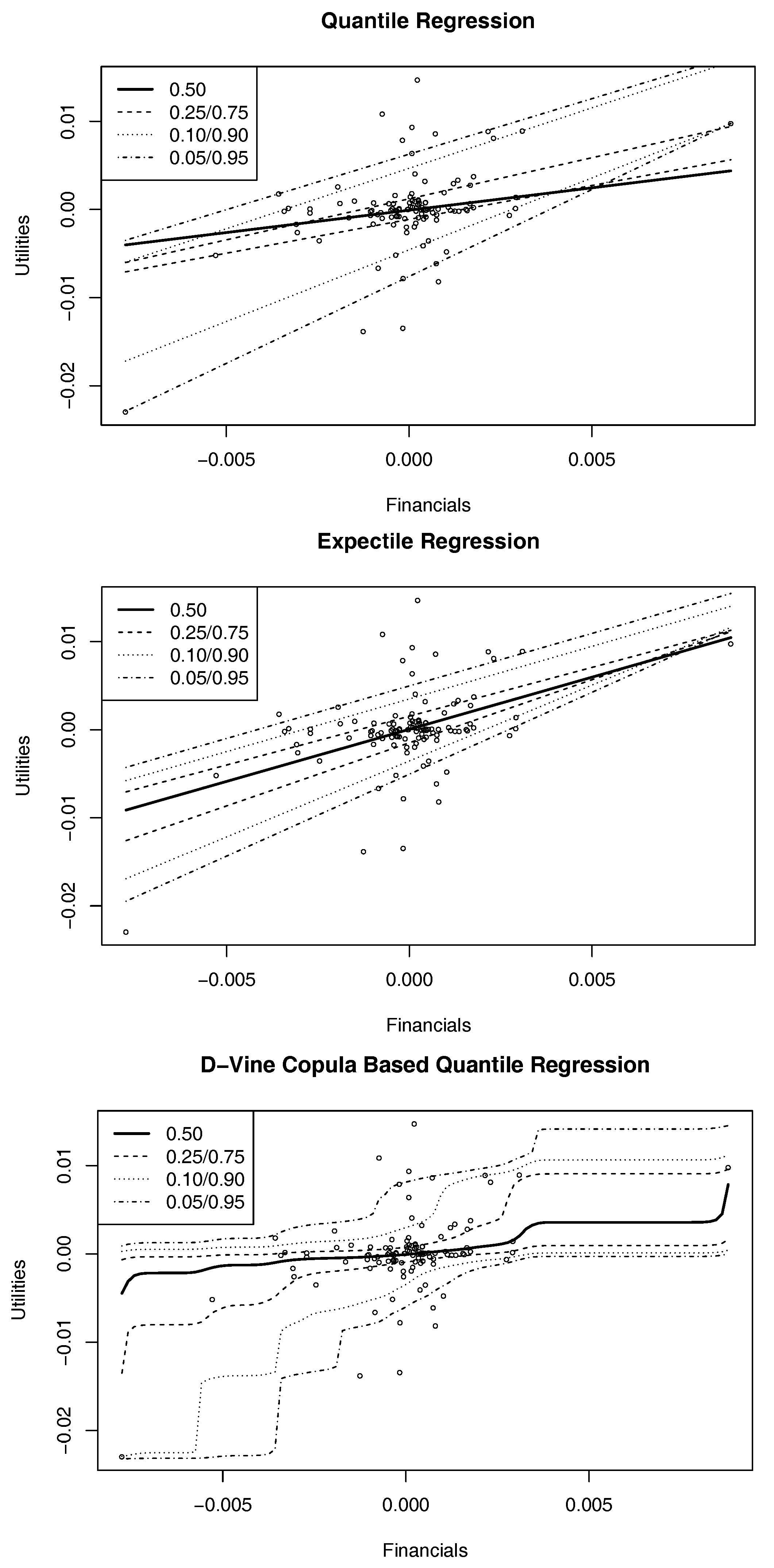
can also be linearly modeled by traditional quantile regression, see e.g., Koenker (2006) and for an example Figure 6 where the method is applied to the differenced time series of response sector Utilities and the covariate Financials, i.e., a two-dimensional model. However, as the conditional quantiles at different levels and are estimated independently it can occur that for given covariate realizations and levels , can have a larger value than , an effect known as quantile crossing. Whereas different approaches have already been proposed to combat quantile crossing, see, e.g., He (1997), Dette and Volgushev (2008) or Bondell et al. (2010), the novel D-vine copula based quantile regression of Kraus and Czado (2017a) also ensures that this effect is prevented.
Expectile regression might be an alternative to quantile regression and has gained increasing attention in the recent literature, see, e.g., Waltrup et al. (2015). Based on replacing the L1 weighting scheme for conditional quantiles by an L2 metric, expectiles
can be bijectively linked to conditional quantiles and also uniquely determine a distribution function. Same as for quantile regression, expectile regression can lead to crossing of estimated curves, see the middle panel of Figure 6. Even though this problem is in practice less likely for expectile regression than for quantile regression, see e.g., Schnabel (2011), similar methods as for regularizing traditional quantile regression can be applied to prevent this effect. Although expectile regression implies some advantages such as computational efficiency, it still bears the problem of weak interpretability. Except for the 50% expectile which can be interpreted as a mean parameter, all other expectiles do not follow an intuitive interpretation in contrast to quantiles. As a consequence, modeling the 50% expectile is equivalent to applying a traditional linear model.
Due to the intuitive interpretability of quantiles over expectiles and the robustness of the median over a mean parameter, we favor quantile regression over expectile regression in this work. Moreover, following the criticism in Bernard and Czado (2015) that conditional quantiles are only linear given very strong assumptions on the underlying copula of the response and covariate variables as well as the quantile crossing problem, we identify the D-vine copula based quantile regression approach as a suitable method for our stress test, see the lower panel of Figure 6.
4. Summary and Outlook
This work evaluates the mutual impact of industry sector specific stress in the German economy using D-vine copula based quantile regression. Concerning simultaneous consideration of covariate and response variables, we illustrate the impact of sector stress arising from Basic Materials, Cyclical Consumer Goods or Industrials on the other industry segments. Above that, our analyses confirm that the Automobile sector strongly influences the whole economy. We also identify that a stressed Financials sector has only moderate influence on the other German industry. Similarly, lagged covariate segments exhibit only minor impact on their response sectors as well. We identify D-vine copula based quantile regression as a preferable method for conducting industry sector stress tests as it accounts for the nonlinearity properties of conditional quantiles and prevents quantile crossing effects. Moreover, in contrast to modeling conditional expectiles, conditional quantiles allow for an intuitive interpretation and have better robustness properties.
Acknowledgments
The authors would like to thank two anonymous referees for their thorough review. We highly appreciate the comments and suggestions which significantly contributed to the quality of this publication.
Author Contributions
Matthias Fischer primarily focused on stress implementation and interpretation, Daniel Kraus on the D-vine copula based quantile regression approach, Marius Pfeuffer on the comparison against alternatives to this method and Claudia Czado on time dependencies and marginal distributions of the data set.
Conflicts of Interest
The authors declare no conflict of interest.
References
- Aas, Kjersti, Claudia Czado, Arnoldo Frigessi, and Henrik Bakken. 2009. Pair-copula constructions of multiple dependence. Insurance, Mathematics and Economics 44: 182–98. [Google Scholar]
- Bedford, Tim, and Roger M. Cooke. 2002. Vines: A new graphical model for dependent random variables. Annals of Statistics 30: 1031–68. [Google Scholar] [CrossRef]
- Bernard, Carole, and Claudia Czado. 2015. Conditional quantiles and tail dependence. Journal of Multivariate Analysis 138: 104–26. [Google Scholar] [CrossRef]
- Bondell, Howard D., Brian J. Reich, and Huixia Wang. 2010. Noncrossing quantile regression curve estimation. Biometrika 97: 825–38. [Google Scholar] [CrossRef] [PubMed]
- Chernozhukov, Victor. 2005. Extremal quantile regression. Annals of Statistics 33: 806–39. [Google Scholar] [CrossRef]
- Chernozhukov, Victor, Iván Fernández-Val, and Tetsuya Kaji. 2017. Extremal quantile regression: An overview. In Handbook of Quantile Regression. Edited by Victor Chernozhukov, Roger Koenker, Xuming He and Limin Peng. London: Chapman & Hall/CRC. [Google Scholar]
- Covas, Francisco B., Ben Rump, and Egon Zakrajšek. 2014. Stress-testing US bank holding companies: A dynamic panel quantile regression approach. International Journal of Forecasting 30: 691–713. [Google Scholar] [CrossRef]
- Dette, Holger, and Stanislav Volgushev. 2008. Non-crossing non-parametric estimates of quantile curves. Journal of the Royal Statistical Society: Series B 70: 609–27. [Google Scholar]
- Fischer, Matthias, Christian Köck, Stephan Schlüter, and Florian Weigert. 2009. An empirical analysis of multivariate copula models. Quantitative Finance 9: 839–54. [Google Scholar] [CrossRef]
- Frahm, Gabriel, Markus Junker, and Alexander Szimayer. 2003. Elliptical copulas: Applicability and limitations. Statistics & Probability Letters 63: 275–86. [Google Scholar]
- He, Xuming. 1997. Quantile curves without crossing. The American Statistician 51: 186–92. [Google Scholar]
- Hobæk Haff, Ingrid, Kjersti Aas, and Arnonldo Frigessi. 2010. On the simplified pair-copula construction—Simply useful or too simplistic? Journal of Multivariate Analysis 101: 1296–310. [Google Scholar] [CrossRef] [Green Version]
- Joe, Harry. 1997. Multivariate Models and Multivariate Dependence Concepts. Boca Raton: CRC Press. [Google Scholar]
- Killiches, Matthias, Daniel Kraus, and Claudia Czado. 2017. Examination and visualisation of the simplifying assumption for vine copulas in three dimensions. Australian & New Zealand Journal of Statistics 59: 95–117. [Google Scholar]
- Koenker, Roger. 2006. Quantile regresssion. Encyclopedia of Environmetrics. [Google Scholar] [CrossRef]
- Koenker, Roger, and Zhijie Xiao. 2002. Inference on the quantile regression process. Econometrica 70: 1583–612. [Google Scholar] [CrossRef]
- Kraus, Daniel, and Claudia Czado. 2017a. D-vine copula based quantile regression. Computational Statistics and Data Analysis 110C: 1–18. [Google Scholar]
- Kraus, Daniel, and Claudia Czado. 2017b. Growing simplified vine copula trees: Improving Dißmann’s algorithm. arXiv, arXiv:arXiv:1703.05203. [Google Scholar]
- McNeil, Alexander J., and Johanna Nešlehová. 2009. Multivariate archimedean copulas, d-monotone functions and l-norm symmetric distributions. The Annals of Statistics 37: 3059–97. [Google Scholar] [CrossRef]
- Merton, Robert C. 1974. On the pricing of corporate debt: The risk structure of interest rates. The Journal of Finance 29: 449–70. [Google Scholar]
- Nelsen, Roger B. 2006. An Introduction to Copulas, 2nd ed. New York: Springer Science + Business Media. [Google Scholar]
- Ong, Ms Li L. 2014. A Guide to IMF Stress Testing: Methods and Models. Washington: International Monetary Fund. [Google Scholar]
- Schechtman, Ricardo, and Wagner Piazza Gaglianone. 2012. Macro stress testing of credit risk focused on the tails. Journal of Financial Stability 8: 174–92. [Google Scholar] [CrossRef]
- Schnabel, S.K. 2011. Expectile Smoothing: New Perspectives on Asymmetric Least Squares. An Application to Life Expectancy. Ph. D. thesis, Utrecht University, Utrecht, The Netherlands. [Google Scholar]
- Sklar, A. 1959. Fonctions dé repartition á n dimensions et leurs marges. Publications de l’Institut de Statistique de l’Université de Paris 8: 229–31. [Google Scholar]
- Spanhel, Fabian, and Malte S. Kurz. 2015. Simplified vine copula models: Approximations based on the simplifying assumption. arXiv, arXiv:arXiv:1510.06971. [Google Scholar]
- Stöber, Jakob, Harry Joe, and Claudia Czado. 2013. Simplified pair copula constructions—Limitations and extensions. Journal of Multivariate Analysis 119: 101–18. [Google Scholar] [CrossRef]
- Waltrup, Linda Schulze, Fabian Sobotka, Thomas Kneib, and Goran Kauermann. 2015. Expectile and quantile regression—David and Goliath? Statistical Modelling 15: 433–56. [Google Scholar] [CrossRef]
Figure 1.
Exemplary plot of the mean probability of default in the industry sector Financials.
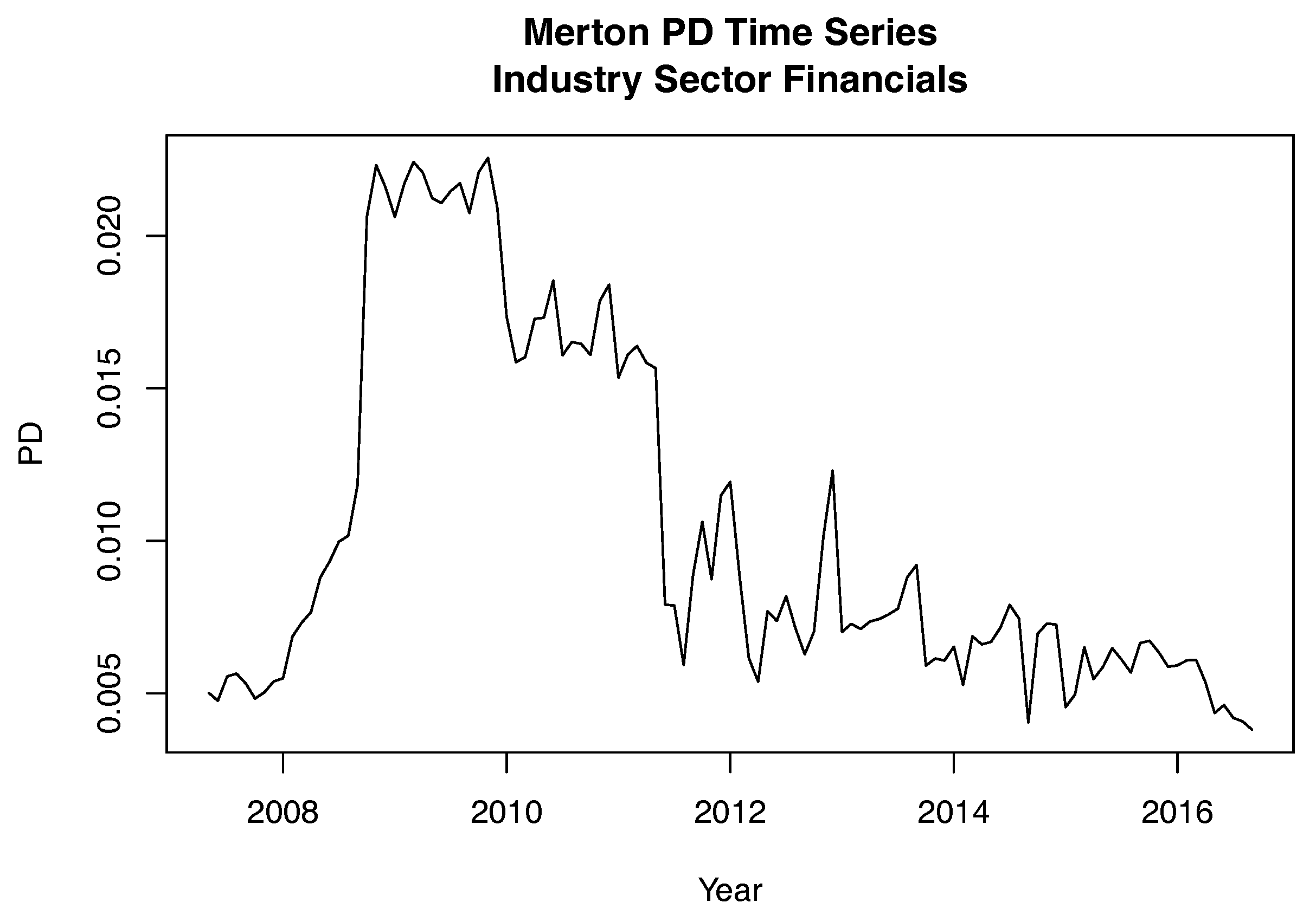
Figure 2.
Histograms of monthly differences of the aggregated sector probabilities of default (PDs).
Figure 2.
Histograms of monthly differences of the aggregated sector probabilities of default (PDs).

Figure 3.
Upper triangular matrix: scatter plots with standard normal margins and Kendall’s values between pairs of aggregated sectors. Lower triangular matrix: contour plots of densities of pairs of aggregated sectors based on empirical copulas and standard normal margins. Diagonal: histograms of marginals after transformation to the copula scale.

Figure 4.
Stress testing results for selected industry sectors. In each plot, the sector written in bold italics is stressed at levels 95% (black) and 99% (gray). The brackets indicate the 95% prediction interval.
Figure 4.
Stress testing results for selected industry sectors. In each plot, the sector written in bold italics is stressed at levels 95% (black) and 99% (gray). The brackets indicate the 95% prediction interval.

Figure 5.
Results of stressing the sub-sectors Basic Materials (left) and the Automobile Industry (right). The bold italic sub-sectors are stressed at level 95%.
Figure 5.
Results of stressing the sub-sectors Basic Materials (left) and the Automobile Industry (right). The bold italic sub-sectors are stressed at level 95%.
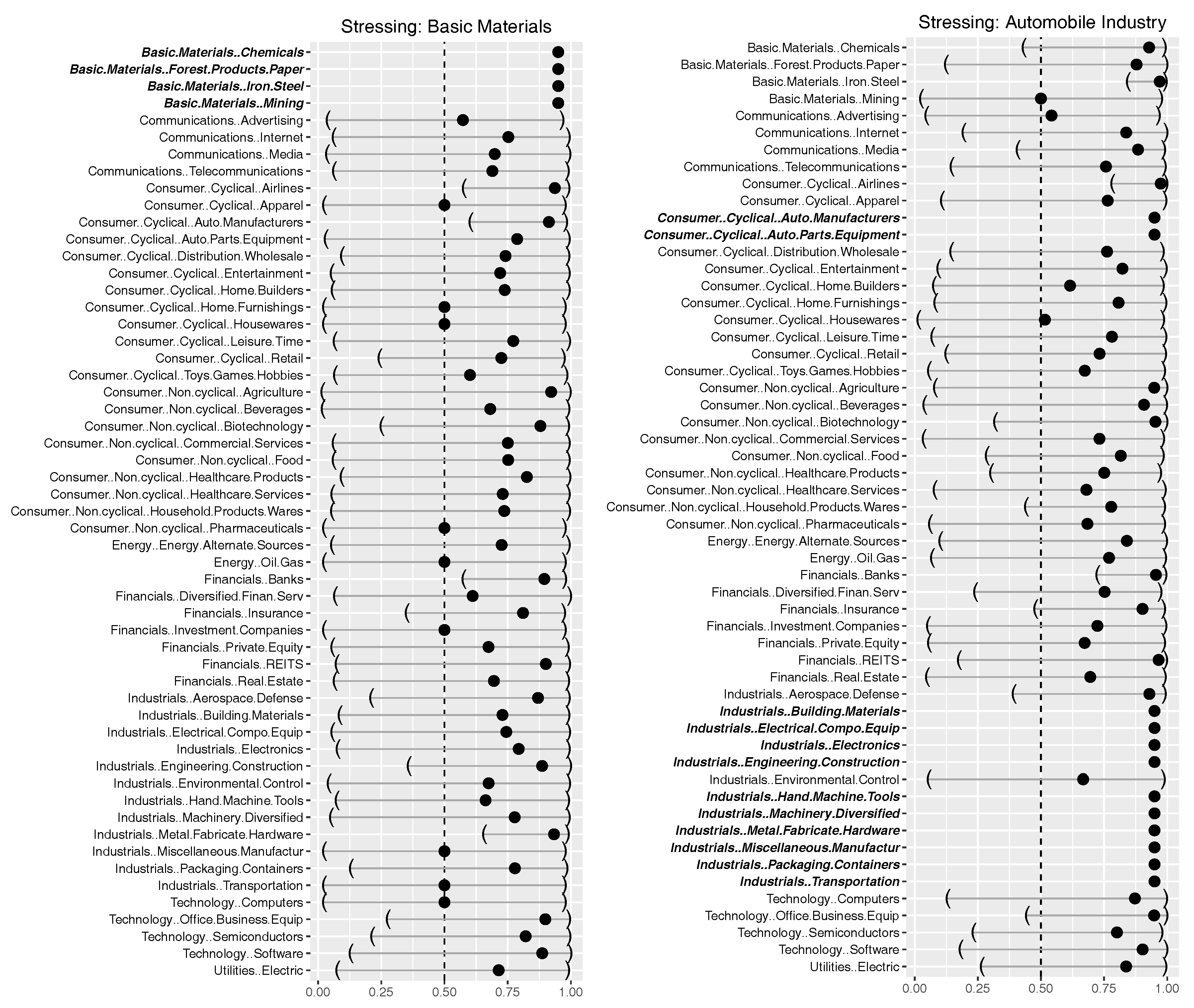
Figure 6.
Estimated curves of regressing the differenced PDs of Utilities against the different PDs of Financial using linear quantile regression (upper panel), expectile regression (middle panel) and D-vine copula based quantile regression (lower panel) for different levels of .
Figure 6.
Estimated curves of regressing the differenced PDs of Utilities against the different PDs of Financial using linear quantile regression (upper panel), expectile regression (middle panel) and D-vine copula based quantile regression (lower panel) for different levels of .

© 2017 by the authors. Licensee MDPI, Basel, Switzerland. This article is an open access article distributed under the terms and conditions of the Creative Commons Attribution (CC BY) license (http://creativecommons.org/licenses/by/4.0/).
Share and Cite
MDPI and ACS Style
Fischer, M.; Kraus, D.; Pfeuffer, M.; Czado, C. Stress Testing German Industry Sectors: Results from a Vine Copula Based Quantile Regression. Risks 2017, 5, 38. https://doi.org/10.3390/risks5030038
AMA Style
Fischer M, Kraus D, Pfeuffer M, Czado C. Stress Testing German Industry Sectors: Results from a Vine Copula Based Quantile Regression. Risks. 2017; 5(3):38. https://doi.org/10.3390/risks5030038
Chicago/Turabian StyleFischer, Matthias, Daniel Kraus, Marius Pfeuffer, and Claudia Czado. 2017. "Stress Testing German Industry Sectors: Results from a Vine Copula Based Quantile Regression" Risks 5, no. 3: 38. https://doi.org/10.3390/risks5030038
Note that from the first issue of 2016, this journal uses article numbers instead of page numbers. See further details here.