
The Class of (p,q)-spherical Distributions with an Extension of the Sector and Circle Number Functions


University of Rostock, Institute of Mathematics, Ulmenstraße 69, Haus 3, 18057 Rostock, Germany
Risks 2017, 5(3), 40; https://doi.org/10.3390/risks5030040
Submission received: 24 May 2017
/
Revised: 17 July 2017
/
Accepted: 19 July 2017
/
Published: 21 July 2017
Abstract
:For evaluating the probabilities of arbitrary random events with respect to a given multivariate probability distribution, specific techniques are of great interest. An important two-dimensional high risk limit law is the Gauss-exponential distribution whose probabilities can be dealt with based on the Gauss–Laplace law. The latter will be considered here as an element of the newly-introduced family of -spherical distributions. Based on a suitably-defined non-Euclidean arc-length measure on -circles, we prove geometric and stochastic representations of these distributions and correspondingly distributed random vectors, respectively. These representations allow dealing with the new probability measures similarly to with elliptically-contoured distributions and more general homogeneous star-shaped ones. This is demonstrated by the generalization of the Box–Muller simulation method. In passing, we prove an extension of the sector and circle number functions.
Keywords:
Gauss-exponential distribution; Gauss–Laplace distribution; stochastic vector representation; geometric measure representation; (p,q)-generalized polar coordinates; (p,q)-arc length; dynamic intersection proportion function; (p,q)-generalized Box–Muller simulation method; (p,q)-spherical uniform distribution; dynamic geometric disintegration1. Introduction
The Gauss-exponential distribution plays an important role as a high risk limit law; see Sections 8 and 9 of the lectures presented in Balkema and Embrechts (2007) on high risk scenarios and extremes. Needless to recall here are the numerous different fields where quantitative risk management applies. The Gauss-exponential distribution can be considered as a particular asymmetric derivation of the Gauss–Laplace law. In particular, Gauss-exponential probabilities of arbitrary events can be dealt with by considering the corresponding Gauss–Laplace probabilities. Density level sets of the standard Gauss–Laplace distribution are topological boundaries of star bodies centered at the origin. The Minkowski functionals of the corresponding star bodies, however, are not homogeneous functions of order one, as is often assumed in the literature on star-shaped distributions. Instead, the bodies corresponding to different density levels reflect different geometric properties and are typically directed in different directions. The aim of the present paper is to model -spherical generalizations of the two-dimensional Gauss–Laplace distribution. We prove geometric and stochastic representations, which can be considered as standard tools for dealing with the present distributions later on in a way similar to how one has already for a long time successfully been dealing with elliptically-contoured and, since more recently, even with more general homogeneous star-shaped distributions. This will be shortly indicated here by generalizing the Box–Muller simulation method.
It is well known from two-dimensional spherical distribution theory that a random vector X following such distribution allows a stochastic representation with independent non-negative random variable R and singular (with respect to the Lebesgue measure in ) random vector U being uniformly distributed on the Euclidean unit circle. Understanding the suitable way of generalizing the latter distribution requires the most effort in general homogeneous star-shaped distribution theory. The corresponding singular distribution is dealt with by several authors (even in higher dimensions) by considering densities of marginal variables (vectors); see (Yue and Ma 1995) and (Song and Gupta 1997) for the particular case of -spherical distributions. Studying a disintegration formula for this case, it is proven in (Rachev and Rueschendorf 1991) that the geometric surface measure cannot coincide with their uniform distribution if . Moreover, the authors mention that ‘its treatment seems to need a completely different proof than the proof for the uniform distribution given in this (their) paper.’ In (Schechtman and Zinn 1990), the authors exploit properties of the distribution being called the uniform distribution on -spheres in (Rachev and Rueschendorf 1991), by making use of a representation of it later called a cone measure representation; see (Barte et al. 2005). An insightful Kepler law interpretation of this measure is discussed in (Wallen 1995). A coordinate-based approach to describing uniform distributions on -spheres is given in (Szablowski 1998) where it is inter alia said that ‘it seems that the usage of the word uniform’ ... ’ does not refer to the real, geometrical uniformity of the probability mass on the surface of the unit sphere in n-dimensional ’. The differential geometric explanation of the generalized uniform distribution given for the particular case of -spheres for arbitrary finite dimension in Richter (2009) (and for dimension two already in two earlier papers on the circle number function mentioned there) provided a qualitatively new approach to this long standing measure theoretical problem. Elliptically contoured and more general homogeneous star-shaped distributions are studied analogously in (Richter 2011a, 2013, 2014, 2015a, 2015b, 2016a, 2016b) based on the consideration of suitably-introduced non-Euclidean geometries.
Much effort is expected to be necessary to give a suitable explanation of the geometric nature of a uniform distribution in the present case that the Minkowski functional of the density contour sets defining the star body is not homogeneous of order one. In going through all of the necessary steps to reach such an interpretation, we will be confronted with generalizing the notions of circle and its radius, as well as its circumference and with an extension of the sector and circle number functions. In the homogeneous case, that is if the mentioned Minkowski functional is homogeneous of order one, the analogous steps can be observed in Richter (2007) and in the author’s series of papers mentioned before. Even more information on the history of the mentioned measure theoretical problem can be found there.
Among others, a technical key role will be played here by the suitable choice of coordinates for describing generalized uniform distributions. Moreover, we make a next basic step of extending the sector and circle number functions to classes of generalized circles having different geometric properties for different values of their generalized radii.
The density of the standard Gauss–Laplace law in is given by:
Let us consider the -spherical generalized normal density:
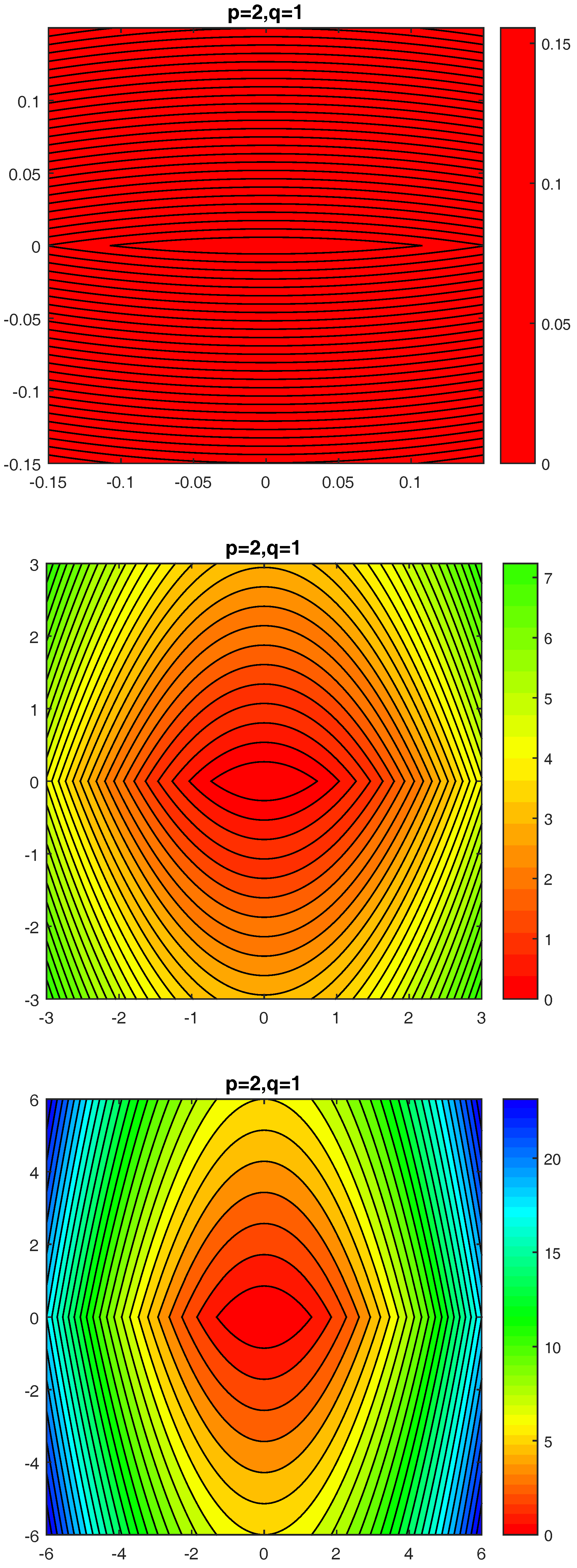
where , and . We note that and and are two-dimensional standard Gauss and Laplace distribution laws, respectively. Figure 1 shows -spherical densities for different choices of .
The case has been considered elsewhere, and we emphasize that this case will not be dealt with in the present paper. Thus, is assumed here. Let:
denote the functional generating the density level sets or contour lines:
Such a level set can be generated from the -generalized unit circle by matrix multiplication:
and will be called the -circle of -radius r. Here, with denoting the diagonal matrix with diagonal entries a and b. The star body:
having the origin in its interior and as its topological boundary will be called the -circle disc of -radius r. It satisfies the subset relation:
and allows the representation:
Such a disc is convex if and and is radially concave if and . For the latter notion, we refer to (Moszyńska and Richter 2012). Figure 2 (drawn with MATLAB, as Figure 1) shows -circles according to different values of the -generalized radius r, starting from a local (central) and turning to more global view. Roughly said, the impression of the main orientation of density level lines is changing within two steps from ‘west-east’ to ‘south-north’.
The paper is organized as follows. Section 2 presents preliminary material on -generalizations of the common polar coordinates, the notions of arc-length and geometric disintegration, the sector and circle number functions and the generalized uniform distribution on a generalized circle. After further developing the general methodology from the theory of homogeneous star-shaped distributions, we are in a position to formally introduce the family of -spherical distributions in Section 3 including the -generalized normal distributions as particular cases of such distributions having a density. Section 4 deals with a geometric generalization of the asymmetric Gauss-exponential law, and Section 5 is devoted to some aspects of simulation. The discussion in Section 6 delivers a look back to and ahead toward the present distribution theory. Finally, we give some conclusions in Section 7.
2. Preliminaries
2.1. A Class of -Generalized Polar Coordinates
Definition 1.
The -generalized polar, or -spherical, coordinate transformation:
is defined by where:
Lemma 1.
The absolute value of the Jacobian of this transformation is:
where:
2.2. The -arc Length Measure and Dynamic Geometric Disintegration of the Lebesgue Measure
In this section, first, the -generalized arc length and the area content of -circles and -circle discs are introduced, respectively. Then, a new type of geometric disintegration of the Lebesgue measure will be established. In the next section, extensions of the sector and circle number functions are considered. To start with, we recall that the area content of the -circle disc with -generalized radius is:
Successively changing variables and shows that:
We note that the power exponent of reflects a certain aspect of the change of shape of when varies. Moreover, we emphasize the remarkable differences between convex and radially-concave cases. In the sequel, in a certain analogy to what was done in (Richter 2007, 2009, 2011b, 2013)for various situations, we define the -generalized arc length measure on the Borel -field of . To this end, for an arbitrary set , let us call:
a nonlinear matrix transformed central projection cone. Note that if and that if . The set can be considered as a union of pairwise disjoint sets,
Here, multiplication of a set by a matrix is defined in the common pointwise sense. Furthermore, a -sector of having -generalized radius r is defined by:
and we consider the -radius dependent area content function:
Here, , and denotes the inverse function of .
Definition 2.
The -arc length measure is defined for arbitrary by:
It follows from the definition of f that:
and:
In particular,
If has finite area content, then:
Because if and only if , it follows that:
where:
denotes the -spherical intersection proportion function of the set B. By similar argumentation, the following theorem is proven. We note that (7) represents a new non-Euclidean type of geometric disintegration of the Lebesgue measure in , which due to the effects of action will be called a dynamic disintegration. For this reason, the function in (8) will be called a dynamic intersection proportion function, and the integration method in (7) will be called dynamic geometric disintegration of the Lebesgue measure.
Theorem 1.
If h is integrable over B, then the dynamic geometric disintegration:
is valid where:
2.3. The -Circle and Sector Number Functions
Circle numbers of star discs are studied in Richter (2011b) and for particular cases in earlier papers cited therein. Similarly, we define the -circle number function to assign the number to any -circle of -radius r where for any :
As for any ,
we can also define the -sector number function to assign the number to any -sector of -radius r where:
and:
In particular, the -circle number allows the following integral representations:
thus:
Moreover,
To summarize some results from this and the last sections for the case , that is for the case being of particular interest when considering the Gauss–Laplace law, we have seen that:
2.4. The -Spherical Uniform Distribution
The -arc length measure introduced in Section 2.2 will be used now to define the generalized (non-Euclidean) uniform distribution on a -circle.
Definition 3.
The -spherical uniform probability law on the Borel σ-field is defined by:
This relative arc-length measure appears to be quite natural. To see this, let be a probability space; a random vector follows the common uniform distribution on the -circle disc ,
and be the -radius of X. Excepting the origin, every point from the interior of belongs just to one of the -circles ; thus, for every , there is a uniquely-defined , such that:
Theorem 2.
The random vector follows the -spherical uniform distribution on and is independent of the random variable R, and R has the following density with respect to the Lebesgue measure on the real line:
Proof.
The cumulative distribution function of R is:
thus the density of R is given by:
Now, let , then:
Because:
it follows that:
Finally,
☐
Remark 1.
If Y is uniform on a -distributed random variable, then follows the distribution having the density in (12).
On the one hand, the -spherical uniform probability distribution is singular with respect to the Lebesgue measure in the two-dimensional Euclidean space but on the other hand, it is absolutely continuous with respect to the Lebesgue measure on the real line. Its density is given therefore by:
that is:
Now, let us define the -spherical sector measure on the Borel -field of as:
According to our consideration in Section 2.3, the -spherical uniform distribution allows the -spherical sector measure and the -arc length representations:
respectively. An additional nonlinear matrix transformed cone measure representation of the -spherical uniform distribution is given by:
3. On the -Spherical Generalization of the Gauss–Laplace Law
The following analogue to Theorem 2 is our starting point for introducing here the new general family of -spherical distributions.
Theorem 3.
Let a random vector follow the -spherical distribution law , and put . The random vector follows the -generalized uniform distribution on and is independent of the random variable R, and R has the density with respect to the Lebesgue measure on the real line:
Proof.
The cumulative distribution function of R is:
Because of:
it follows that:
Furthermore, for
and
☐
Remark 2.
According to Theorem 3, if , then X allows the stochastic representation:
where follows the -spherical uniform distribution, , and R has the density (14) and is independent of .
The following definition is well motivated by Remark 2.
Definition 4.
(a) Let follow the -spherical uniform distribution on the Borel σ-field of the -unit circle , and R a non-negative random variable having cumulative distribution function F and characteristic function ϕ and being independent of , then:
is said to follow the -spherical distribution . The vector is called the -spherical uniform basis and R the generating variate of X. The distribution of X will alternatively be denoted if R has density function f.
(b) An arbitrary random vector X taking values in is called -spherically distributed if there exists a nonnegative random variable R being independent of a -spherical uniformly-distributed random vector U, such that .
Here, means that random vector Y is distributed as random vector Z.
Theorem 4.
The characteristic function of a -spherically distributed random vector X satisfying the representation can be written as:
where and denote the distribution law induced by the random variable R and the characteristic function of the -spherical uniform distribution, respectively.
Proof.
By definition,
thus
Because R and U are independent,
and by Fubini’s theorem,
☐
Corollary 1.
(a) The distribution of a -spherically distributed random vector X is uniquely determined by the distribution of its generating variate R.
(b) If a -spherically distributed random vector X has a density, then it is of the form ,
where is a density generating function (dgf) satisfying:
and the normalizing constant allows the factorization:
Proof.
(a) If with and being independent of U, and , then, by Theorem 4, .
(b) Because the distribution of a -spherically distributed random vector with nonnegative R being independent of U, , is already determined by the distribution of R, the density of X is already determined by the density of R. By Fubini’s theorem,
☐
In what follows, we denote the distribution law of a -spherically distributed random vector having dgfg by . The following theorem deals with a geometric representation of such measures.
Theorem 5.
For every ,
Proof.
Because of: ,
Since if and only if , it follows that:
☐
The geometric measure representation in Theorem 5 will be called a dynamic geometric disintegration of the -spherical measure .
Corollary 2.
Let and . Then, R follows the density:
Proof.
Let . Theorem 5 applies with , and R follows the density:
☐
Finally, we note that Corollary 2 generalizes Formula (14). That is, if in Corollary 2, then and
4. Asymmetric -Spherical Generalization of the Gauss-Exponential Law
The Gauss-exponential density and the Gauss–Laplace density are connected through the equation . Accordingly, the Gauss-exponential probability of an arbitrary random event from can be dealt with by doubling the corresponding Gauss–Laplace probability. Therefore, the Gauss-exponential law can be considered as an asymmetric derivation of the Gauss–Laplace law.
In (Balkema and Embrechts 2007), the exponential component of the Gauss-exponential distribution law arises when a Gaussian vector is subject to a certain conditioning process assuming that this vector belongs to a half space having a positive distance from the origin. As one result of this conditioning process, the domain of definition of a multivariate distribution is restricted to a proper subset. If the conditioning process were to be modified, other asymmetric distributions derived from the Gauss–Laplace law could be of interest.
The possible consequences on the geometric measure representation of a multivariate star-shaped distribution law caused by a restriction of the domain of definition to a proper subset are described in Remark 1 in Richter (2015b). A similar approach can be of interest here.
The two-dimensional exponential distribution may be considered as a restriction of the distribution with (not considered here) to the domain of definition . For a geometric generalization of the multivariate exponential law, we refer to the class of regular simplicially contoured or -norm symmetric distributions studied in (Henschel and Richter 2002). Further results for p-spherical distributions with p from can be found in (Rachev and Rueschendorf 1991), (Kamiya et al. 2008) and (Richter and Schicker 2016).
5. Simulation
First of all, we recall that the radius component of a uniformly on distributed random vector can be simulated according to Remark 1. Numerous others generalized radius distributions may be simulated using various particular methods.
The well-known simulation method in (Box and Muller 1958) was extended to the p-generalized normal distribution in (Kalke and Richter 2013). Similarly, here, we establish a simulation method for arbitrary -spherically distributed vectors. According to Theorem 2, the vector follows, independently of the variable R, the -spherical uniform distribution on ,
By (13), the density of angle is given as:
Starting from this representation, one can proceed as described in (Kalke and Richter 2013) and Richter (2015a), Example 9(b), or any of the standard monographs on simulation mentioned there.
6. Discussion
The way of probabilistic modeling developed in this paper is closely related to various challenging mathematical problems. It is well known from the results in (Richter 2014, 2016a, 2016b) and the references given there that representations of star-shaped distributions whose contour-defining star body has a homogeneous Minkowski functional of order one are closely related to suitably-chosen non-Euclidean geometries. Here, we discover that there is again a need to go some steps beyond such geometries and realize the first of them.
Already in the 17th Century, basically starting from the work of Descartes, various coordinate systems played a fruitful role in geometric applications. Nevertheless, it seems that suitably chosen coordinates may serve even these days as a powerful tool for solving nontrivial problems in different areas of mathematics. In the present case, star bodies whose Minkowski functionals are not homogeneous functions of degree one are effectively described for the purposes of representing two-dimensional Gauss–Laplace laws and their -spherical generalizations with the help of generalized polar coordinates based on generalized sine and cosine functions.
Starting latest from the work of Leibniz and Newton who founded modern calculus, in many areas of mathematics, one makes use of thin parallel layers when defining and studying certain basic notions. Here, however, small changes of a generalized radius variable related to such a body generate thin layers close to the bodies’ boundary, being nonparallel. To the best of the author’s knowledge, the fundamental measure theoretical problem of understanding the factorization components of cross-sections or disintegrations of the present type seems to be approached here for the first time.
The present work extends the line of interchanging the role that the notions of circle and distance play in comparison with Euclidean geometry, described inter alia in (Richter 2011a, 2011b). Here, the ‘circle’ is given by a density level set modeling a ‘contour line’ of a sample cloud, and the understanding of what is a ‘distance’ leads to a directionally-dependent notion of radius being related to a matrix-vector multiplication. This remains, however, that the question of what is the differential geometric meaning of the newly-introduced -generalized arc length measure. Therefore, it is stated here as an open problem.
Finally, we remark that the results in Section 2 allow the following additional representations of the Lebesgue measure, which may be useful in future applications of -spherical distributions. For ,
and for ,
An alternative representation is given for by:
7. Conclusions
The Gauss-exponential distribution being of particular interest in high risk scenarios can be numerically dealt with now based upon a method newly developed in this paper. This method, moreover, opens new perspectives for studying in the future broad classes of multivariate distributions not just being homogeneous of order one. A detailed and full developement of this distribution theory will further bring together methods at least from measure theory, non-Euclidean differential geometry, isoperimetry, extending ball and sector number functions, defining suitable coordinates, solving partial differential equations, and functional analysis.
Conflicts of Interest
The author declares no conflict of interest.
References
- Balkema, Guus, and Paul Embrechts. 2007. High Risk Scenarios and Extremes. In Zurich Lectures in Advanced Mathematics. Zurich: European Mathematical Society. [Google Scholar]
- Barte, Franck, Olivier Guédon, Shahar Mendelson, and Assaf Naor. 2005. A probabilistic approach to the geometry of the -ball. Annals of Probability 33: 480–513. [Google Scholar] [CrossRef]
- Box, George E.P., and Mervin E. Muller. 1958. A note on the generation of random normal deviates. The Annals of Mathematical Statistics 29: 610–11. [Google Scholar] [CrossRef]
- Henschel, Volkmar, and Wolf-Dieter Richter. 2002. Geometric generalization of the exponential law. Journal of Multivariate Analysis 81: 189–204. [Google Scholar] [CrossRef]
- Kalke, Steve, and Wolf-Dieter Richter. 2013. Simulation of the p-generalized Gaussian distribution. Journal of Statistical Computation and Simulation 83: 639–65. [Google Scholar] [CrossRef]
- Kamiya, Hidehiko, Akimichi Takemura, and Satoshi Kuriki. 2008. Star-shaped distributions and their generalizations. Journal of Statistical Planning and Inference 138: 3429–47. [Google Scholar] [CrossRef]
- Moszyńska, Maria, and Wolf-Dieter Richter. 2012. Reverse triangle inequality. Antinorms and semi-antinorms. Studia Scientiarum Mathematicarum Hungarica 49: 120–38. [Google Scholar] [CrossRef]
- Rachev, Svetlozar T., and L. Ruschendorf. 1991. Approximate independence of distributions on spheres and their stability properties. The Annals of Probability 19: 1311–37. [Google Scholar] [CrossRef]
- Richter, Wolf-Dieter. 2007. Generalized spherical and simplicial coordinates. Journal of Mathematical Analysis and Applications 336: 1187–202. [Google Scholar] [CrossRef]
- Richter, Wolf-Dieter. 2009. Continuous -symmetric distributions. Lithuanian Mathematical Journal 49: 93–108. [Google Scholar] [CrossRef]
- Richter, Wolf-Dieter. 2011a. Circle numbers for star discs. ISRN Geometry. [Google Scholar] [CrossRef]
- Richter, Wolf-Dieter. 2011b. Ellipses numbers and geometric measure representations. Journal of Applied Analysis 17: 165–79. [Google Scholar] [CrossRef]
- Richter, Wolf-Dieter. 2013. Geometric and stochastic representations for elliptically contoured distributions. Communications in Statistics: Theory and Methods 42: 579–602. [Google Scholar] [CrossRef]
- Richter, Wolf-Dieter. 2014. Geometric disintegration and star-shaped distributions. Journal of Statistical Distributions and Applications 1: 20. [Google Scholar] [CrossRef]
- Richter, Wolf-Dieter. 2015a. Norm contoured distributions in . Lecture Notes of Seminario Interdisciplinare di Mathematica 12: 179–99. [Google Scholar]
- Richter, Wolf-Dieter. 2015b. Convex and radially concave contoured distributions. Journal of Probability and Statistics. [Google Scholar] [CrossRef]
- Richter, Wolf-Dieter. 2016a. Star-shaped distributions: Euclidean and non-Euclidean representations. In Proceedings of the 60th ISI World Statistics Congress, Rio de Janeiro, Brazil, 26–31 July 2015. [Google Scholar]
- Richter, Wolf-Dieter. 2016b. Representing continuous star-shaped probability measures in spaces with suitably constructed geometries. AIP Conference Proceedings 1738: 190002. [Google Scholar] [CrossRef]
- Richter, Wolf-Dieter, and Kay Schicker. 2016. Circle numbers of regular convex polygons. Results in Mathematics 69: 521–38. [Google Scholar] [CrossRef]
- Schechtman, Gideon, and Joel Zinn. 1990. On the volume of intersection of two Lnp balls. Proceedings of the American Mathematical Society 110: 217–24. [Google Scholar]
- Song, Danhong, and Arjun K. Gupta. 1997. Lp-norm uniform distributions. Proceedings of the American Mathematical Society 125: 595–601. [Google Scholar] [CrossRef]
- Szablowski, Pawel J. 1998. Uniform distributions on spheres in finite dimensional lα and their generalizations. Journal of Multivariate Analysis 64: 103–17. [Google Scholar] [CrossRef]
- Wallen, Lawrence J. 1995. Kepler, the taxicab metric, and beyond: An isoperimetric primer. The College Mathematics Journal 26: 178–90. [Google Scholar] [CrossRef]
- Yue, Xinnian, and Chunsheng Ma. 1995. Multivariate lp-norm symmetric distributions. Statistics and Probability Letters 24: 281–88. [Google Scholar] [CrossRef]
Figure 1.
-spherical densities.
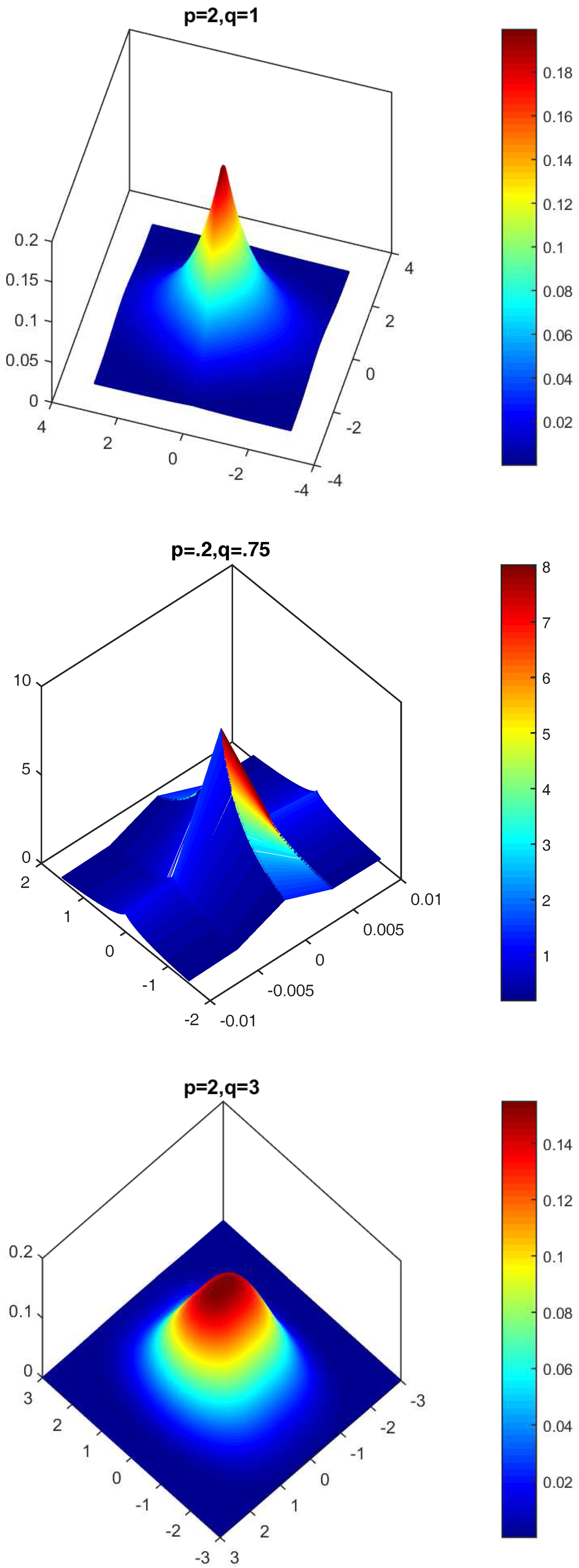
Figure 2.
Gauss–Laplace density level sets: from local (central) to global view.

© 2017 by the author. Licensee MDPI, Basel, Switzerland. This article is an open access article distributed under the terms and conditions of the Creative Commons Attribution (CC BY) license (http://creativecommons.org/licenses/by/4.0/).
Share and Cite
MDPI and ACS Style
Richter, W.-D. The Class of (p,q)-spherical Distributions with an Extension of the Sector and Circle Number Functions. Risks 2017, 5, 40. https://doi.org/10.3390/risks5030040
AMA Style
Richter W-D. The Class of (p,q)-spherical Distributions with an Extension of the Sector and Circle Number Functions. Risks. 2017; 5(3):40. https://doi.org/10.3390/risks5030040
Chicago/Turabian StyleRichter, Wolf-Dieter. 2017. "The Class of (p,q)-spherical Distributions with an Extension of the Sector and Circle Number Functions" Risks 5, no. 3: 40. https://doi.org/10.3390/risks5030040
Note that from the first issue of 2016, this journal uses article numbers instead of page numbers. See further details here.