
Existence and Uniqueness for the Multivariate Discrete Terminal Wealth Relative


Institute for Mathematics, RWTH Aachen University, Templergraben 55, D-52062 Aachen, Germany
*
Author to whom correspondence should be addressed.
Risks 2017, 5(3), 44; https://doi.org/10.3390/risks5030044
Submission received: 5 May 2017
/
Revised: 12 August 2017
/
Accepted: 25 August 2017
/
Published: 28 August 2017
Abstract
:In this paper, the multivariate fractional trading ansatz of money management from Vince (Vince 1990) is discussed. In particular, we prove existence and uniqueness of an “optimal f” of the respective optimization problem under reasonable assumptions on the trade return matrix. This result generalizes a similar result for the univariate fractional trading ansatz. Furthermore, our result guarantees that the multivariate optimal f solutions can always be found numerically by steepest ascent methods.
1. Introduction
Risk and money management for investment issues has always been at the heart of finance. Going back to the 1950s, Markowitz (1991) invented the “modern portfolio theory”, where the additive expectation of a portfolio of different investments was maximized subject to a given risk expressed by volatility of the portfolio.
When the returns of the portfolio are no longer calculated additive, but multiplicative in order to respect the needs of compound interest, the resulting optimization problem is known as “fixed fractional trading”. In fixed fractional trading strategies an investor always wants to risk a fixed percentage of his current capital for future investments given some distribution of historic trades of his trading strategy.
A first example of factional trading was established in the 1950s by (Kelly 1956) who found a criterion for an asymptotically optimal investment strategy for one investment instrument. Similarly, Vince in the 1990s (see (Vince 1990, 1992)) used the fractional trading ansatz to optimize his position sizing. Although at first glance these two methods look quite different, they are in fact closely related as could be shown in (Maier-Paape 2016). However, only recently (Vince 2009) extended the fractional trading ansatz to portfolios of different investment instruments. The situation with M investment instruments (systems) and N coincident realizations of absolute returns of these M systems results in a trade return matrix T described in detail in (2). Given this trade return matrix, the “Terminal Wealth Relative” (TWR) can be constructed (see (4)) measuring the multiplicative gain of a portfolio resulting from a fixed vector of fractional investments into the M systems. In order to find an optimal investment among all fractions the TWR has to be maximized
where is the definition set of the TWR (see Definition 1 and (8)).
Whereas (Vince 2009) only stated this optimization problem and illustrated it with examples, in Section 3 we give as our main result the necessary analysis. In particular, we investigate the definition set of the TWR and fix reasonable assumptions (Assumption 1) under which (1) has a unique solution. This unique solution may lie in or on as different examples in Section 4 show. Our result extend the results of (Maier-Paape 2013; Zhu 2007) ( case only) and parts of the PhD of (Hermes 2016) on the discrete multivariate TWR. One of the main ingredients to show the uniqueness of the maximum of (1) is the concavity of the function (see Lemma 5). Uniqueness and concavity furthermore guarantee that the solution of (1) can always be found numerically by simply following steepest ascent.
Before we start our analysis, some more remarks on related papers are in order. In (Maier-Paape 2015) showed that the fractional trading ansatz on one investment instrument leads to tremendous drawdowns, but that effect can be reduced largely when several stochastic independent trading systems are used coincidentally. Under which conditions this diversification effect works out in the here considered multivariate TWR situation is still an open question. Furthermore, several papers investigated risk measures in the context of fractional trading with one investment instrument (; see (De Prado et al. 2013; Maier-Paape 2013, 2016; Vince and Zhu 2013)). Related investigations for the multivariate TWR using the drawdown can be found in (Vince 2009).
In the following sections, we analyse the multivariate case of a discrete Terminal Wealth Relative. That means we consider multiple investment strategies where every strategy generates multiple trading returns. As noted before this situation can be seen as a portfolio approach of a discrete Terminal Wealth Relative (cf. (Vince 2009)). For example, one could consider an investment strategy applied to several assets, the strategy producing trading returns on each asset. However, in an even broader sense, one could also consider several distinct investment strategies applied to several distinct assets or even classes of assets.
2. Definition of a Terminal Wealth Relative
The subject of consideration in this paper is the multivariate case of the discrete Terminal Wealth Relative for several trading systems analogous to the definition of Ralph Vince in (Vince 2009). For we denote the k-th trading system by (system k). A trading system is an investment strategy applied to a financial instrument. Each system generates periodic trade returns, e.g., monthly, daily or the like. The absolute trade return of the i-th period of the k-th system is denoted by , . Thus, we have the joint return matrix
and define
Just as in the univariate case (cf. (Maier-Paape 2013) or (Vince 1990)), we assume that each system produced at least one loss within the N periods. That means
Thus, we can define the biggest loss of each system as
For better readability, we define the rows of the given return matrix, i.e., the return of the i-th period, as
and the vector of all biggest losses as
Having the biggest loses at hand, it is possible to “normalize” the k-th column of T by such that each system has a maximal loss of . Using the componentwise quotient, the normalized trade matrix return then has the rows
For , , we define the Holding Period Return (HPR) of the i-th period as
where denotes the standard scalar product on . To shorten the notation, the marking of the vector space at the scalar product is omitted, if the dimension of the vectors is clear. Similar to the univariate case, the gain (or loss) in each system is scaled by its biggest loss. Therefore the HPR represents the gain (loss) of one period, when investing a fraction of of the capital in () for all , thus risking a maximal loss of in the k-th trading system.
The Terminal Wealth Relative (TWR) as the gain (or loss) after the given N periods, when the fraction is invested in () over all periods, is then given as
Note that in the –dimensional case a risk of a full loss of our capital corresponds to a fraction of . Here in the multivariate case we have a loss of of our capital every time there exists an such that . That is for example if we risk a maximal loss of in the -th trading system (for some ) and simultaneously letting for all other . However these degenerate vectors of fractions are not the only examples that produce a Terminal Wealth Relative (TWR) of zero. Since we would like to risk at most of our capital (which is quite a meaningful limitation), we restrict to the domain given by the following definition:
Definition 1.
A vector of fractions is called admissible if holds, where
Furthermore, we define
With this definition we now have a risk of for each vector of fractions and a risk of less than for each vector of fractions . Since
we can find an such that
and thus in particular holds. denotes the Euclidean norm on .
Observe that the i-th period results in a loss if , that means . Hence the biggest loss over all periods for an investment with a given vector of fractions is
Consequently, we have a biggest loss of
and
Note that for we do not have an a priori bound for the fractions . Thus it may happen that there are with for some (or even for all) , or at least , indicating a risk of more than for the individual trading systems, but the combined risk of all trading systems can still be less than . So the individual risks can potentially be eliminated to some extent through diversification. As a drawback of this favorable effect the optimization in the multivariate case may result in vectors of fractions that require a high capitalization of the individual trading systems. Thus, we assume leveraged financial instruments and ignore margin calls or other regulatory issues.
Before we continue with the TWR analysis, let us state a first auxiliary lemma for .
Lemma 1.
The set in Definition 1 is convex, as is .
Proof.
All the conditions and
define half spaces (which are convex). Since is the intersection of a finite set of half spaces, it is itself convex.
A similar reasoning yields that is convex, too. ☐
3. Optimal Fraction of the Discrete Terminal Wealth Relative
If we develop this line of thought a little further a necessary condition for the return matrix T for the optimization of the Terminal Wealth Relative gets clear:
Lemma 2.
Assume there is a vector with then
If in addition there is an such that then
Proof.
If
it follows that
For arbitrary the function
is monotonically increasing in s for all and by that we have
Moreover, if there is an with then
and by that
An investment where the holding period returns are greater than or equal to 1 for all periods denotes a “risk free” investment () and considering the possibility of an unbounded leverage, it is clear that the overall profit can be maximized by investing an infinite quantity. Assuming arbitrage free investment instruments, any risk free investment can only be of short duration, hence by increasing the condition will eventually burst, cf. (7). Thus, when optimizing the Terminal Wealth Relative , we are interested in settings that fulfill the following assumption
always yielding .
With that at hand, we can formulate the optimization problem for the multivariate discrete Terminal Wealth Relative
and analyze the existence and uniqueness of an optimal vector of fractions for the problem under the assumption
Assumption 1.
We assume that each of the trading systems in (2) produced at least one loss (cf. (3)) and furthermore
- (a)
- (b)
- (c)
Assumption 1(a) ensures that, no matter how we allocate our portfolio (i.e., no matter what direction we choose), there is always at least one period that realizes a loss, i.e., there exists an with . Or in other words, not only are the investment systems all fraught with risk (cf. (3)), but there is also no possible risk free allocation of the systems.
The matrix T from (2) can be viewed as a linear mapping
“” denotes the kernel of the matrix T in Assumption 1(c). Thus, this assumption is the linear independence of the trading systems, i.e., the linear independence of the columns
of the matrix T. Hence with Assumption 1(c) it is not possible that there exists an and a such that
which would make () obsolete. So Assumption 1(c) is no actual restriction of the optimization problem.
Now we point out a first property of the Terminal Wealth Relative.
Lemma 3.
Let the return matrix (as in (2)) satisfy Assumption 1(a) then, for all , there exists an such that . In fact .
Proof.
For some arbitrary we have . Then Assumption 1(a) yields the existence of an with . With
and
we get that
and for all . Hence and clearly (cf. Definition 1). ☐
Furthermore, the following holds.
Lemma 4.
Let the return matrix (as in (2)) satisfy Assumption 1(a) then the set is compact.
Proof.
For all Assumption 1(a) yields an such that . With that we define
This function is continuous on the compact support . Thus, the maximum exists
Consequently the function
is well defined and continuous. Since for all
with equality for at least one index , we have
and
hence
Altogether we see that
thus the set is bounded and connected as image of the compact set under the continuous function g and by that the set is compact. ☐
Now we take a closer look at the third assumption for the optimization problem.
Lemma 5.
Let the return matrix (as in (2)) satisfy Assumption 1(c) then is concave on . Moreover if there is a with , then is even strictly concave in .
Proof.
For the gradient of is given by the column vector
where . The Hessian-matrix is then given by
where is a row vector. The matrix can be rearranged as
Since the matrices are positive semi-definite for all , the same holds for and therefore is concave. Furthermore, if there is a with
where , the matrix further reduces to
If is not strictly positive definite there is a such that
and we get that
yielding a non trivial element in and thus contradicting Assumption 1(c). Hence matrix is strictly positive definite and is strictly concave in . ☐
With this at hand we can state an existence and uniqueness result for the multivariate optimization problem.
Theorem 2. (optimal f existence)
Given a return matrix as in (2) that fulfills Assumption 1, then there exists a solution of the optimization problem (8)
Furthermore, one of the following statements holds:
- (a)
- is unique, or
- (b)
- .
For both cases , and hold true.
Proof.
We show existence and partly uniqueness of a maximum of the N-th root of , yielding existence and partly uniqueness of a solution of (10) with the claimed properties.
With Lemmas 1 and 4, the support of the Terminal Wealth Relative is convex and compact. Hence the continuous function attains its maximum on . For we get from (9)
which is a vector whose components are strictly positive due to Assumption 1(b). Therefore is not a maximum of and a global maximum reaches a value greater than
Since for all
holds, a maximum can not be attained in either.
Now if there is a maximum on , assertion (b) holds together with the claimed properties. Alternatively, a maximum is attained in the interior . In this case, Lemma 5 yields the strict concavity of at . Suppose there is another maximum then the straight line connecting both maxima
is fully contained in the convex set (cf. Lemma 1). Because of the concavity of all points of L have to be maxima, which is a contradiction to the strict concavity of in . Thus, the maximum is unique and assertion (a) holds together with the claimed properties. ☐
In the remainder of this section, we will further discuss case (b) in Theorem 2. We aim to show that the maximum is unique either, but we proof this using a completely different idea. In order to lay the grounds for this, first, we give a lemma:
Lemma 6.
If from (2) is a return map satisfying Assumption 1 and if , then each return map , which results from T after eliminating one of its columns, is also a return map satisfying Assumption 1.
Proof.
Since each of the M trading systems of the return matrix has a biggest loss , , the same holds for the trading systems of the reduced matrix .
For , Assumption 1(b),(c) follow straight from the respective properties of the matrix T.
Now let, without loss of generality, be the matrix that results from T by eliminating the last column, i.e., the M-th trading system is omitted. Let , , denote the rows of and the vector of biggest losses of . Then for Assumption 1(a) we have to show that
such that
Having this at hand, we can now extend Theorem 2.
Corollary 1. (optimal f uniqueness)
In the situation of Theorem 2 the uniqueness also holds for case (b), i.e., a maximum is also a unique maximum of in .
Proof.
Assume that the optimal solution is not unique, then there exists an additional optimal solution with . Since is convex (c.f. Lemma 1), the line connecting both solutions
is fully contained in . Because of the concavity of on (c.f. Lemma 5), all points on L are optimal solutions. Therefore L must be a subset of , since we have seen that an optimal solution in the interior would be unique. Hence, there is (at least) one such that, for all investment vectors in L, the trading system () is not invested. i.e., the -th component of , of and of all vectors in L is zero.
Without loss of generality, let . Then
are two optimal solutions for
However, with that, the -dimensional investment vectors are two distinct optimal solutions for
With Lemma 6 the return map which results from T after eliminating the M-th column (i.e., (system M)) satisfies Assumption 1. Applying Theorem 2 to the sub-dimensional optimization problem, yields that and again lie at the boundary of the admissible set of investment vectors
Hence, we have two distinct optimal solutions on the boundary for the optimization problem with (M−1) investment systems. By induction this reasoning leads to the existence of two distinct optimal solutions for an optimization problem with just one single trading system. However, for that type of problem, we already know that the solution is unique (see for example (Maier-Paape 2013)), which causes a contradiction to our assumption. Thus, also for case (b) we have the uniqueness of the solution . ☐
Remark 1.
Note that Assumption 1(c) is necessary for uniqueness. To give a counterexample imagine a return matrix with two equal columns, meaning the same trading system is used twice. Let be the optimal f for this one dimensional trading system. Then it is easy to see that , and the straight line connecting these two points yield TWR optimal solutions for the return matrix .
4. Examples
As an example we fix the joint return matrix for trading systems and the returns from periods given through the following table.
Obviously every system produced at least one loss within the 6 periods, thus the vector with
is well-defined. For the takes the form
where the set of admissible vectors is given by
Since for all
we have
Accordingly we get
When examining the 6-th row of the matrix we observe that Assumption 1(a) is fulfilled with . To see that let, for some , , then
For Assumption 1(b) one can easily check that all four systems are “profitable”, since the mean values of all four columns in (12) are strictly positive. Lastly, for Assumption 1(c) we check that the rows of matrix are linearly independent
Thus, Theorem 2 yields the existence and uniqueness of an optimal investment fraction with , and , which can numerically be computed
In the above example, a crucial point is that there is one row in the return matrix where the -th entry is the biggest loss of (system k), . Such a row in the return matrix implies, that all trading systems realized their biggest loss simultaneously, which can be seen as a strong evidence against a sufficient diversification of the systems. Hence we analyze Assumption 1(a) a little closer to see what happens if this is not the case.
With the help of Assumption 1(a), for all , there is a row of the return matrix , such that . The sets
describe the hyperplanes generated by the normal direction , . Thus, each from the set has to be an element of one of the half spaces
In other words the set has to be a subset of a union of half spaces
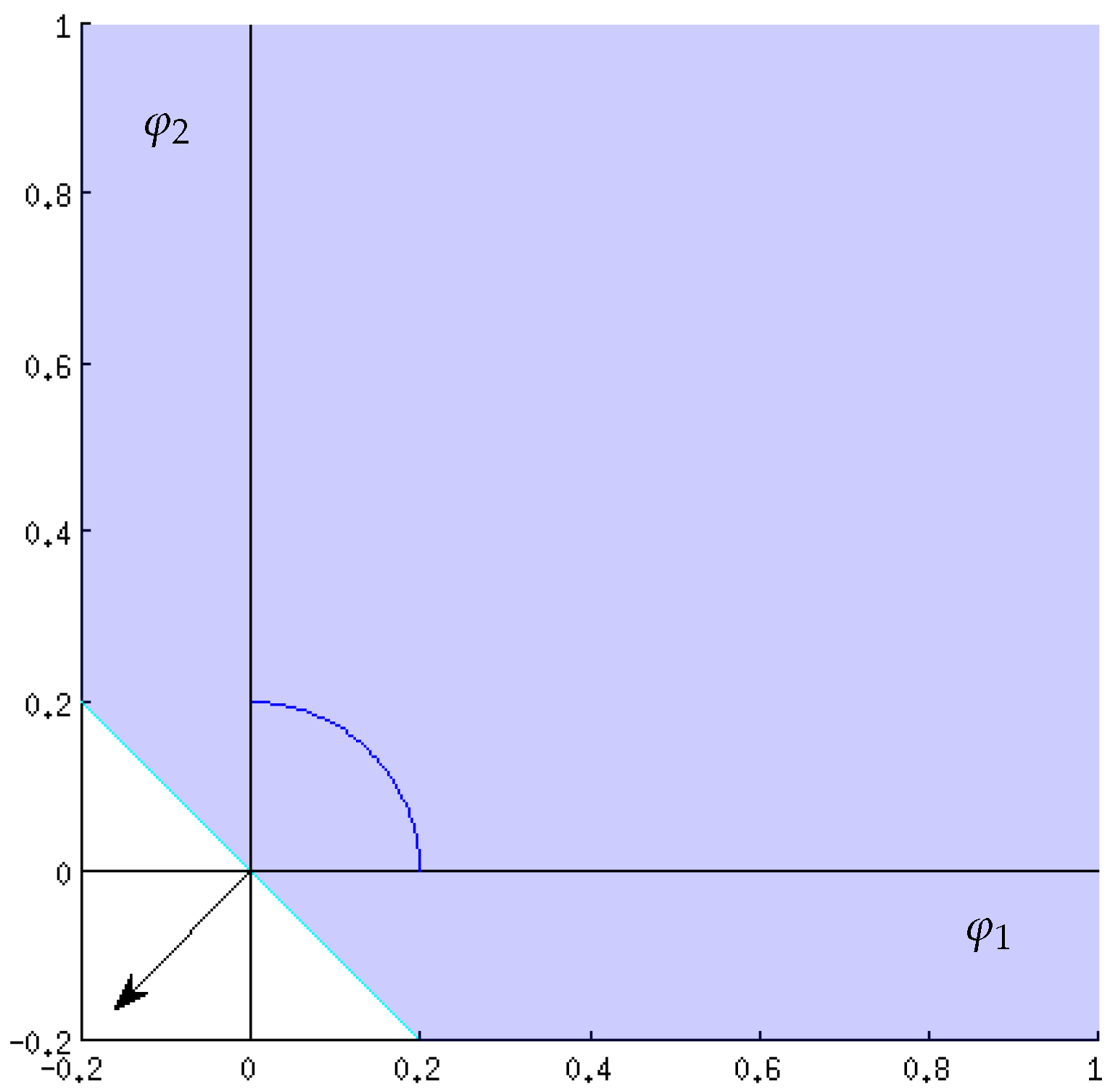
If there exists an index such that for all , then the normal direction of the corresponding hyperplane is
hence
and therefore Assumption 1(a) is fulfilled. Figure 1 shows a hyperplane for and a row of the return matrix where all entries are the biggest losses, that means the normal direction of this hyperplane is the vector
However, it is not necessary for Assumption 1(a) that the set is covered by just one hyperplane. Again for an illustration of possible hyperplanes can be seen in Figure 2. The figure on the left shows a case where Assumption 1(a) is violated and the figure on the right a case where it is satisfied.
Remark 2.
Following our arguments concerning the example in (12) the question arises whether or not a trading system where biggest losses are realized simultaneously always implies insufficient diversification. In (12) this seems to be the case, but is this true in general? One way diversification is often measured in the literature is volatility or variance/standard deviation of the portfolio returns. In terms of modern portfolio theory where portfolios are searched for which either
- minimize risk for a given chance/utility level
- or
- maximize chance/utility for a given risk level,
the volatility stands for the risk part. Transferring this setup for a trade–off between risk and utility to the TWR “utility function” would result in an optimization problem like
where is a constant restricting the risk (or volatility) level and is a symmetric positive definite covariance matrix stemming from a trading game with trade returns as in (2). The optimization problem in (14) is quite similar to the Markowitz portfolio optimization. The only difference is that the Markowitz utility function “expected portfolio return” is exchanged by the concave function .
Since of Theorem 2 solves (10) it is clear that will solve (14) for all . On the other hand, for solutions of (14) will also be “efficient” in this utility/risk setting. However, the volatility decreases as and therefore diversification certainly increases. As a matter of fact, among all efficient portfolios, has the highest volatility and thus the worst diversification. In that sense diversification of is not to be expected.
For the next example we fix the return matrix as
with and . Thus, the biggest losses of the two systems are
To determine the set of admissible investments (and to check Assumption 1) we examine the vectors for
and solve the linear equations
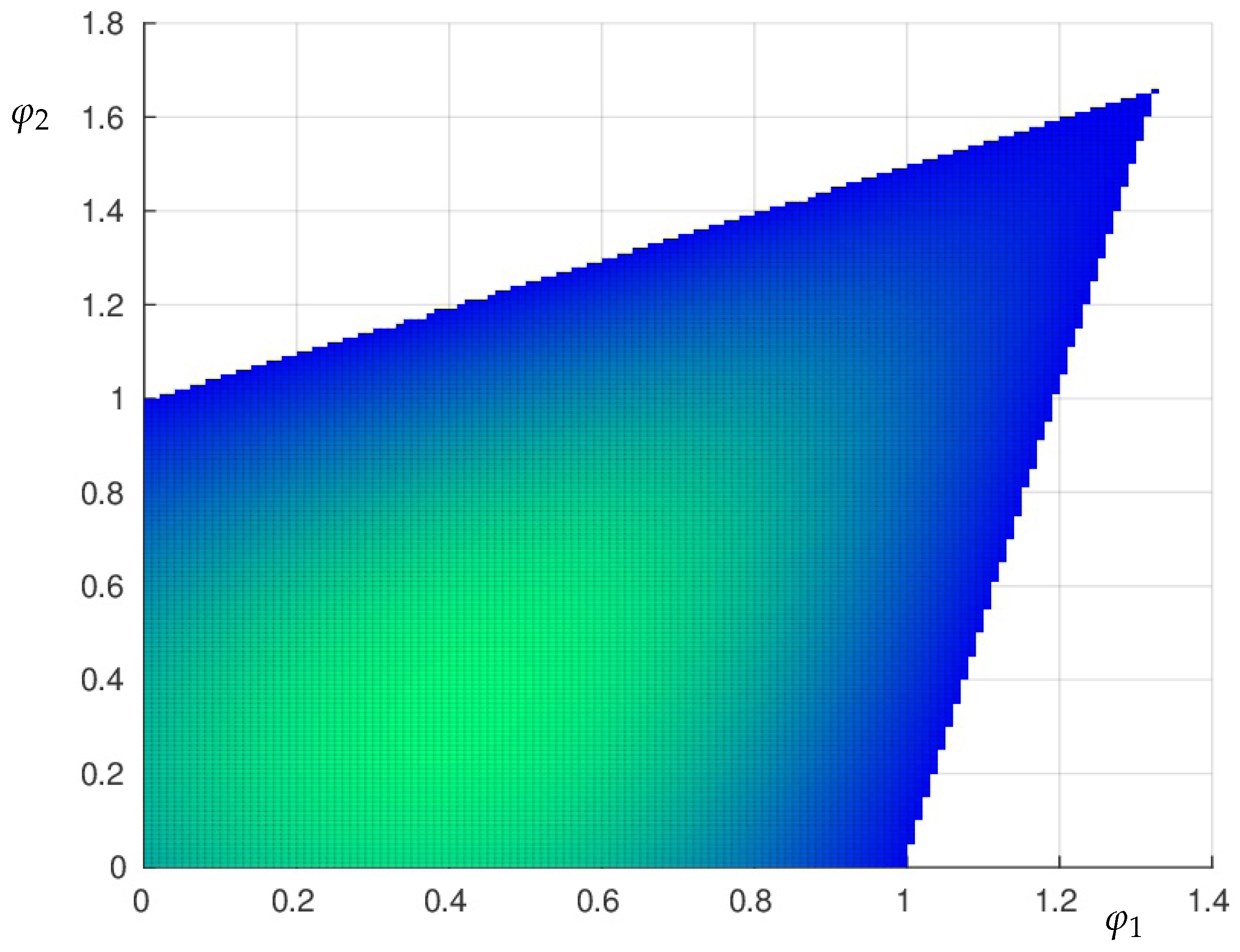
The solutions for are shown in Figure 3.
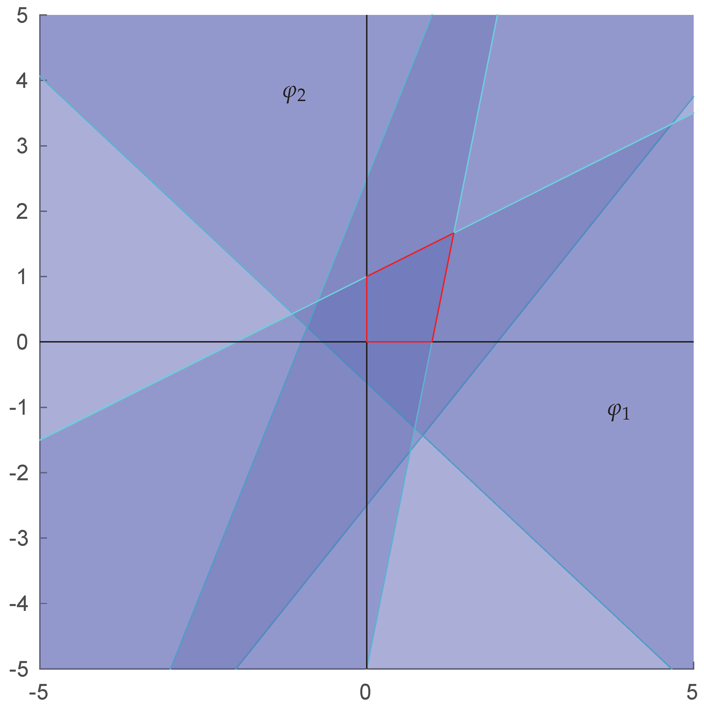
Each solution corresponds to a “cyan” line. The area where the inequality holds for some is shaded in “light blue”. The set where the inequalities hold for all is the section where all shaded areas overlap, thus the “dark blue” section. Therefore the set of admissible investments is given by
with
Assumption 1 is fulfilled, since
- (a)
- the half spaces for rows 4 and 5 of the return matrix cover the whole set (cf. Figure 2b),
- (b)
- and and
- (c)
- obviously, the columns of the return matrix are linearly independent.
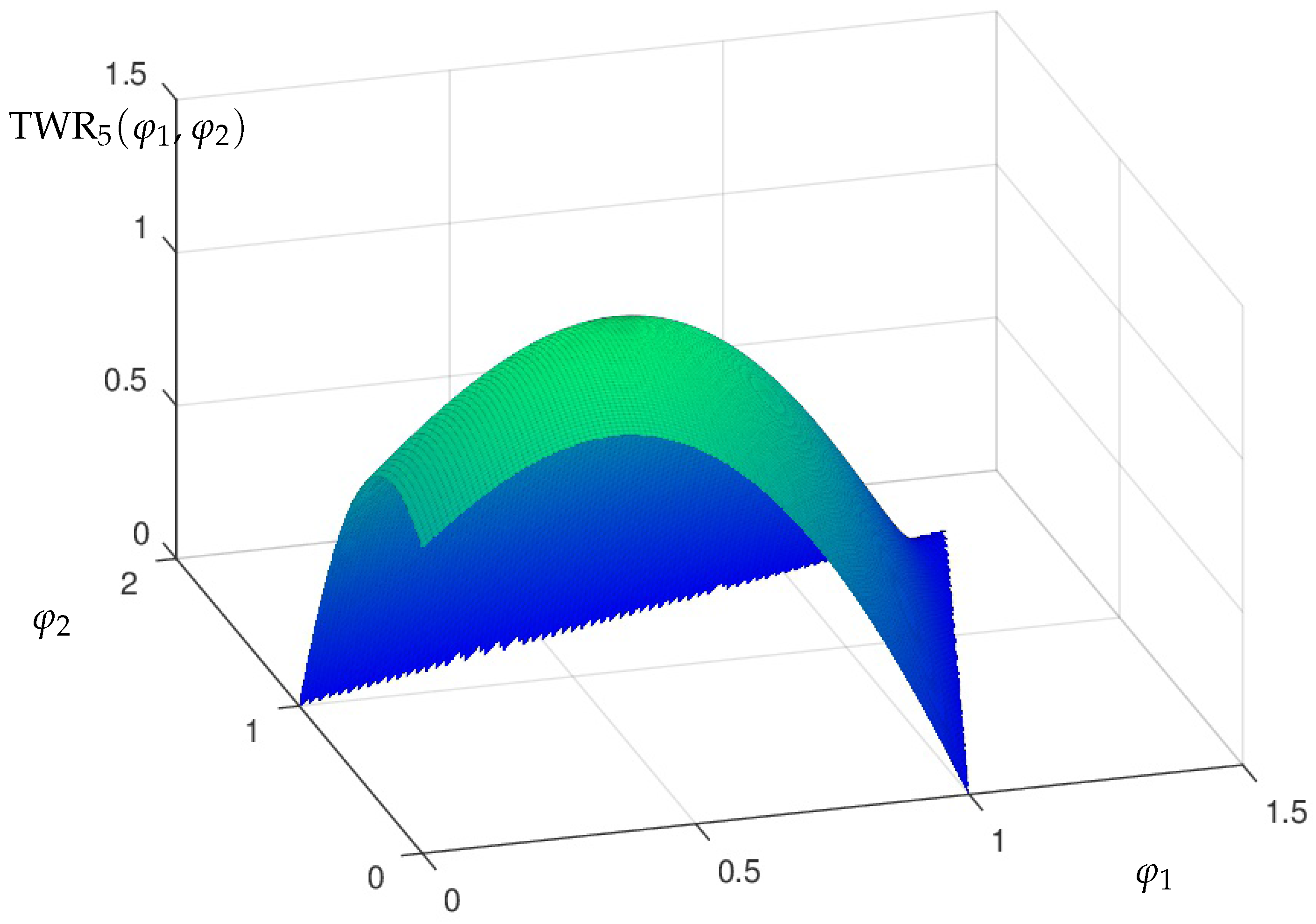
A plot of the Terminal Wealth Relative for the return matrix from (15) can be seen in Figure 4 and Figure 5 with a maximum at
Therefore the maximum is clearly attained in the interior .
The following example will show that the unique maximum of Theorem 2 can indeed be attained on , i.e., the case discussed in Corollary 1. For that we add a third investment system to our last example (16) with the new returns
such that the vectors , , form the matrix
This set of trading systems fulfills Assumption 1(b) since .
Assumption 1(c) is satisfied as well, because the three columns of are linearly independent. For Assumption 1(a) we have to show that
holds. If not, we would have an investment vector
such that (20) is not true for all rows of the matrix . In particular if we look at lines 4 and 5
the sum of both inequalities still has to be true
which is a contradiction to being an element of
Now we examine the following vector of investments
with the unique maximum of the optimization problem of the reduced set of trading systems from the last example (cf. (18)).
The first derivative of the Terminal Wealth Relative in the direction of the third component at is given by
Moreover with being the optimal solution of the last example in two variables we have
and
Thus is indeed a local maximal point on the boundary of for TWR5 with the three trading systems in (19). Corollary 1 yields the uniqueness of this maximal solution for
5. Conclusions
With our main theorems, Theorem 2 and Corollary 1, we were able give a complete existence and uniqueness theory for the optimization problem (8) of a multivariate Terminal Wealth Relative under reasonable assumptions. Furthermore, due to the convexity of the domain (Lemma 1), the concavity of (see Lemma 5) and the uniqueness of the “optimal ” solution, it is always guaranteed that simple numerical methods like steepest ascent will find the maximum.
Author Contributions
The two authors contribute equally to this paper.
Conflicts of Interest
The authors declare no conflict of interest.
References
- Hermes, Andreas. 2016. A Mathematical Approach to Fractional Trading. Ph.D. thesis, RWTH Aachen University, Aachen, North Rhine-Westphalia, Germany. [Google Scholar]
- Kelly, John L., Jr. 1956. A new interpretation of information rate. Bell System Technical Journal 35: 917–26. [Google Scholar] [CrossRef]
- De Prado, Marcos Lopez, Ralph Vince, and Qiji Jim Zhu. 2013. Optimal Risk Budgeting Under a Finite Investment Horizon. Available online: https://papers.ssrn.com/sol3/papers.cfm?abstractid=2364092 (accessed on 1 January 2013).
- Maier-Paape, Stanislaus. 2013. Existence Theorems for Optimal Fractional Trading. Aachen: Institute for Mathematics, RWTH Aachen, report no. 67. [Google Scholar]
- Maier-Paape, Stanislaus. 2015. Optimal f and diversification. International Federation of Technical Analysis Journal 15: 4–7. [Google Scholar]
- Maier-Paape, Stanislaus. 2016. Risk averse fractional trading using the current drawdown. arXiv:1612.02985. [Google Scholar]
- Markowitz, Harry M. 1991. Portfolio Selection. München: FinanzBuch Verlag. [Google Scholar]
- Vince, Ralph. 1990. Portfolio Management Formulas: Mathematical Trading Methods for the Futures, Options, and Stock Markets. Hoboken: John Wiley & Sons, Inc. [Google Scholar]
- Vince, Ralph. 1992. The Mathematics of Money Management, Risk Analysis Techniques for Traders. Hoboken: John Wiley & Sons, Inc. [Google Scholar]
- Vince, Ralph. 2009. The Leverage Space Trading Model: Reconciling Portfolio Management Strategies and Economic Theory. Hoboken: Wiley Trading. [Google Scholar]
- Vince, Ralph, and Qiji Jim Zhu. 2013. Inflection Point Significance for the Investment Size. Available online: https://papers.ssrn.com/sol3/papers.cfm?abstractid=2230874 (accessed on 27 February 2013).
- Zhu, Qiji Jim. 2007. Mathematical analysis of investment systems. Journal of Mathematical Analysis and Applications 326: 708–20. [Google Scholar] [CrossRef]
Figure 1.
Hyperplane for a return vector consisting of “biggest losses”.

Figure 2.
Two hyperplanes and the set .
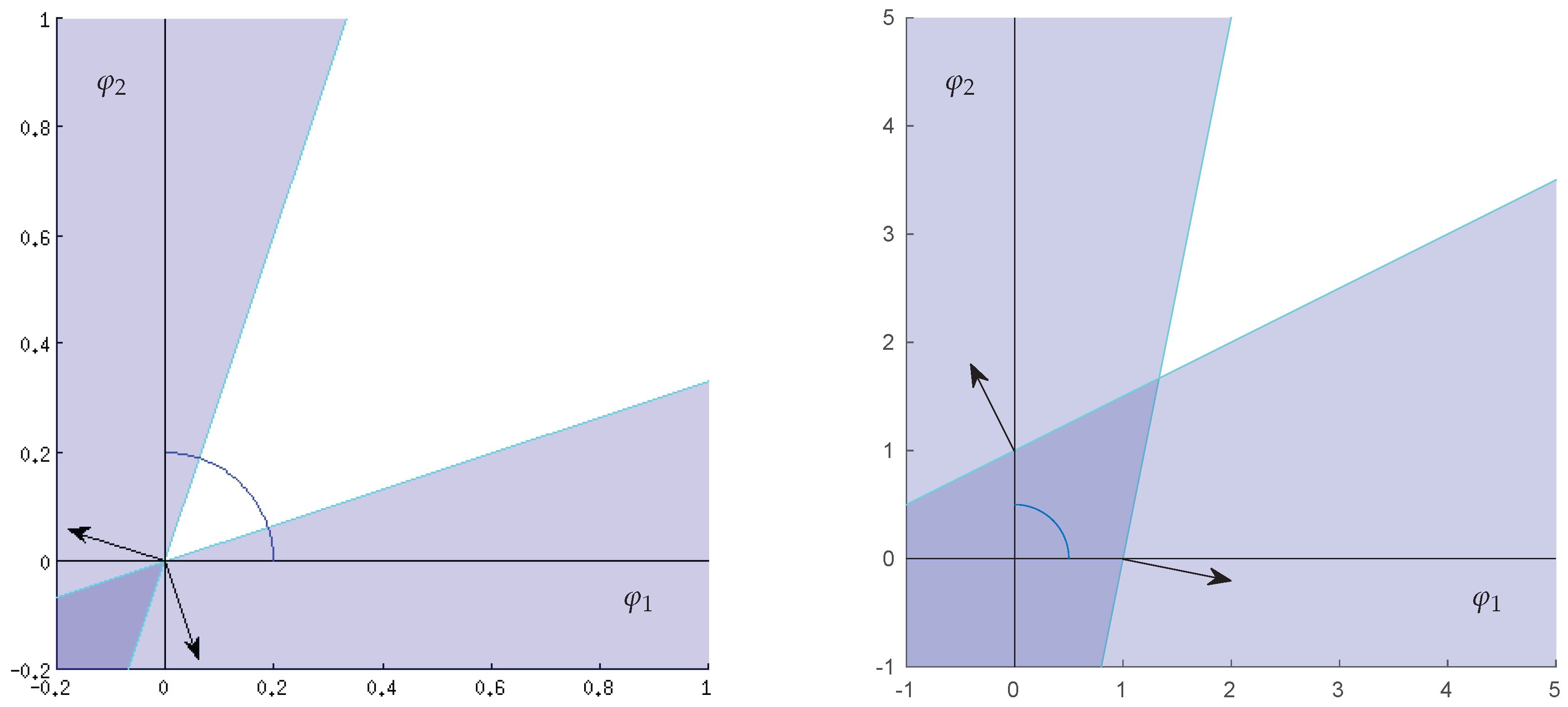
Figure 3.
Solutions of the linear equations from (17).
Figure 3.
Solutions of the linear equations from (17).

Figure 4.
The Terminal Wealth Relative for T from (15).
Figure 4.
The Terminal Wealth Relative for T from (15).

Figure 5.
The Terminal Wealth Relative from Figure 4, view from above.
Figure 5.
The Terminal Wealth Relative from Figure 4, view from above.
© 2017 by the authors. Licensee MDPI, Basel, Switzerland. This article is an open access article distributed under the terms and conditions of the Creative Commons Attribution (CC BY) license (http://creativecommons.org/licenses/by/4.0/).
Share and Cite
MDPI and ACS Style
Hermes, A.; Maier-Paape, S. Existence and Uniqueness for the Multivariate Discrete Terminal Wealth Relative. Risks 2017, 5, 44. https://doi.org/10.3390/risks5030044
AMA Style
Hermes A, Maier-Paape S. Existence and Uniqueness for the Multivariate Discrete Terminal Wealth Relative. Risks. 2017; 5(3):44. https://doi.org/10.3390/risks5030044
Chicago/Turabian StyleHermes, Andreas, and Stanislaus Maier-Paape. 2017. "Existence and Uniqueness for the Multivariate Discrete Terminal Wealth Relative" Risks 5, no. 3: 44. https://doi.org/10.3390/risks5030044
Note that from the first issue of 2016, this journal uses article numbers instead of page numbers. See further details here.