Optimal Claiming Strategies in Bonus Malus Systems and Implied Markov Chains


1
Faculte des Sciences Economiques, Universite Rennes 1, 7 Place Hoche, 35065 Rennes CEDEX, France
2
Batiment Bois de l’Etang, Universite Paris Est, 5 rue Galilee, 77420 Champs sur Marne, France
*
Author to whom correspondence should be addressed.
Risks 2017, 5(4), 58; https://doi.org/10.3390/risks5040058
Submission received: 28 April 2017
/
Revised: 22 September 2017
/
Accepted: 23 October 2017
/
Published: 8 November 2017
Abstract
:In this paper, we investigate the impact of the accident reporting strategy of drivers, within a Bonus-Malus system. We exhibit the induced modification of the corresponding class level transition matrix and derive the optimal reporting strategy for rational drivers. The hunger for bonuses induces optimal thresholds under which, drivers do not claim their losses. Mathematical properties of the induced level class process are studied. A convergent numerical algorithm is provided for computing such thresholds and realistic numerical applications are discussed.
1. Introduction
Bonus-Malus systems are well established tools used in motor insurance pricing based on past experience of drivers. A Bonus—a premium discount (with some lower bound)—is guaranteed by the policy when the driver reports no accident during a predetermined period of time. A Malus— an additional charge to the premium (with some upper bound)—is required when accidents are reported. The obvious purpose of this mechanism is to penalize the bad (or unlucky) drivers and to provide incentives for drivers to try to reduce their claims frequency, as discussed in Franckx (1960) or Hey (1985). From a mathematical perspective, standard Bonus-Malus systems are convenient because they might be modeled using Markov Chains (see Lemaire (1994) and Lemaire (1995b) for a description of various existing systems). Markov Chains properties (and associated invariant measures) can be used to describe the long term equilibrium of the system. But, as a by-product, this mechanism also generates some hunger for bonuses (as described in Lemaire (1977)): drivers might overtake small accidents and not report them to their insurance companies, in order to obtain a reduced premium (and avoid also the additional charge)1. From an empirical perspective, the fact that some accidents might not be reported might be confirmed by the fact that, in many countries with Bonus-Malus schemes, zero-inflated models have a significant ‘zero-component’, as discussed in Boucher et al. (2009), with too many people that do not report claims. In this paper, we exhibit the optimal reporting strategy and address the problem of updating the Markov Chain transition probability of class levels, in order to take into account the probability of not reporting an accident.
1.1. Discrete Bonus-Malus System
The optimal claiming strategy for insured drivers was already addressed in Zachs and Levikson (2004), where a continuous time version of k-class Bonus-Malus systems was considered: drivers are switched to a lower class if no claim were filed during a period T (that might depend on the previous class), while whenever a claim is filed, the insured is immediately switched to a higher level (as in De Pril (1979)). Here, we want to integrate this realistic feature in the more standard approach based on Markov Chains modeling on a finite number of classes, discussed e.g., in Lemaire (1995a), with discrete time (since premium is revised on an annual basis). Here, we intend to incorporate the optimal strategy for drivers not to report a loss whenever the considered amount is too small.
Nevertheless, in a discrete model, if the transition is based on the number of accidents, and not the occurrence (or not) of accidents within a given period (usually one year), modeling hunger for bonus is much more complex. Intuitively, the optimal decision to report and claim a loss is not the same if the policy renewal (and associated premium level update) is either in 360 days, or only in 5 days. Moreover, insured drivers may (and often should) choose to regroup several minor claims and declare them as a large one. In order to avoid those issues and stick to a simple and easily interpretable model, we assume that only one accident per year might occur.
1.2. Advantages of a Discrete Bonus-Malus System
The continuous-time model described in Zachs and Levikson (2004) has nice mathematical properties, but on the other hand discrete-time Bonus-Malus systems are interesting since they are easily interpretable, and can naturally be formalized via Markov Chains. In order to illustrate this our model, let consider a benchmark very simple Bonus-Malus system, with 3 classes, similar to the one discussed in Section 6 of Zachs and Levikson (2004). A different premium is associated to each class , with . If no claim occurs during one year, a driver is upgraded from class i to class , as long as . In case of claim report, the driver is downgraded from class i to class , as long as . See Table 1 for a description of that scheme.
Suppose that accident occurrence is driven by an homogeneous Poisson process, with intensity , given some initial class at time , as in standard actuarial models. Then the trajectory of classes for the driver can be described by a discrete Markov process. If denote the probability to have no accident over a year, the transition probability matrix of the Markov Chain is given by
for the classes 1, 2 and 3 (in that order).
Based on this transition probability matrix, a quantitative figure of interest is the corresponding stationary distribution, describing the repartition of drivers within the classes in a stationary regime. Given this stationary distribution, one can then compute the corresponding average premium in the (long term) stationary state, see e.g., Lemaire (1995b) and related studies. But, unfortunately, this (standard) study of Bonus-Malus schemes is almost always based on the unrealistic assumption that all car accidents are reported to the insurance company. However, it might not be optimal for a client to claim all losses.
For instance, suppose that an insured in class 2 suffers a loss of level ℓ. Then,
- if the loss is claimed, next year premium will be as he will downgrade from class 2 to class 3;
- if the loss is not claimed, he will loose ℓ and next year premium will be , as he will upgrade from class 2 to class 1.
So a basic short term economic reasoning indicates here that it is rational to not to claim a loss as soon as , i.e., . It is common knowledge that this type of reasoning is even suggested by the insurance company, as soon as a driver intends to report a small loss. It indeed happened recently to one of the authors of the paper.
1.3. Towards an Optimal Claiming Strategy
This ‘hunger for bonus’, as defined in Franckx (1960) or Lemaire (1977), can be mathematically formulated as an ‘optimal claiming strategies’, as discussed in Walhin and Paris (1999), Walhin and Paris (2000) and Denuit et al. (2007)—where Chapter 5 is dedicated to that issue.
An over-naive approach sometimes suggested in rather serious newspapers consists in taking into account the impact on all the following years of deciding today to report or not a given accident. Such strategy consists in comparing the sum of all discounted premia, associated to both possible starting class level, depending if the accident is claimed or not. This naive approach does not take into account the set of all possible scenarios associated to the possible random trajectories of the Markov process on the class set . A driver can not be assumed a deterministic trajectory for future Bonus-Malus classes and related premia.
In order to take into account the occurrence of new accidents in the following years, one needs to associate to each class level s and time t, a value combining all the possible future accident scenario costs, whenever starting in class level s at time t. To take into account future scenarios, consider a (discrete) discount rate . Namely, a rational decision is to avoid declaring the accident whenever in class s, as soon as
where the function represents the expected value of all future discounted claims and premia for the driver, whenever he starts from class k at time . This function V must integrate the occurrence of accidents in the future, as well as the corresponding probabilistic evolution of the class-level Markov Chain given , considering that the driver sticks to the optimal reporting strategy designed by (1).
Hence, the optimal claiming strategy rewrites as the solution of an optimal switching control problem, where a driver needs to decide at each time step, if he should claim a possibly occurred accident or not. As detailed above, this decision simply characterizes in terms of the lag between the 2 values assigned to the both possible reachable class level. Claiming an accident will be optimal whenever the cost of the accident exceeds the corresponding so-called implied deductible, as in Braun et al. (2006) and Chappell and Norman (2003).
1.4. Agenda
The main purpose of this paper is to identify the optimal strategy for reporting losses and derive its main mathematical properties as well as a convergent approximating numerical scheme. Applying this optimal reporting strategy, we observe that the corresponding level class process remains a Markov chain, with modified transition probabilities. In Section 2, we formalize the problem of interest and describe the related Markov chains. In Section 3, we derive and characterize the optimal reporting strategy of the driver and provide a simple algorithmic routine to approximate it. The algorithm will in particular be tested in a 5-state Spanish Bonus-Malus scheme, see Section 4. Extensions including the addition of deductibles, as well as the consideration of heterogeneous, or risk adverse, drivers are presented in Section 5.
2. Problem Formulation
2.1. Bonus-Malus Based on Loss Occurrence
Classical Bonus-Malus transition probabilities are usually computed under the assumption that every accident is reported, as in e.g., Lemaire (1995b). This gives rise to a Markov Chain dynamics for the class level of any driver. For example, a standard model for accident occurrence is the Poisson process. With an homogeneous Poisson process, with intensity , the Markov process is also homogenous.
Consider for instance the classical 3-classe Bonus-Malus scheme described in Section 1.2 above. Recall that, in such system, a driver is upgraded whenever no accident occurs and is downgraded at the arrival of any claimed accident, see Table 1. As soon as all losses are claimed to the insurance company, the level-class Markov Chain associated to such Bonus-Malus system has the following transition matrix
where p denotes the probability to have no accident on a one year period. Observe that the probability that a loss occurs does not depend on the class level s. This classical feature is due to the no-memory property of the Poisson process.
In a stationary regime, the invariant probability measure characterizing the repartition of the drivers within the 3 classes is given by
In addition, we deduce the average premium in the stationary regime, which is given by
In the numerical illustration, this asymptotic premium is used in order to enforce actuarial equilibrium between the driver and the insurer in the sense that
where L denotes the (random) loss amount of an accident.
2.2. Impact of Claim Reporting Strategies
Observe that the previous stationary distribution of drivers within classes only depends on the frequency of the loss, via the probability parameter p. In particular, it is not connected to the levels of the premiums or the possible severity of the accident. This feature relies on the fact that we unfortunately did not take into account the economic behavior of drivers, and in particular the fact that they may choose not to report small losses. They shall do this whenever the gain from reporting an accident does not compensate the impact of the class level downgrade on the future premia.
A loss reporting strategy for a driver is hereby given by a collection of thresholds , associated to any class s. Let denote the collection of such strategies, i.e.,
where denotes the collection of class levels. A driver will decide to report a claim while in class s, if and only if the severity of the loss ℓ exceeds the threshold , i.e., if and only if .
The choice of the reporting strategy for the driver has an important impact on the trajectory of his associated class level Markov Chain, that we denote . This can be precisely quantified, as the reporting strategy directly impacts the transition probabilities of the class level Markov Chain . Let indeed denote by the probability to report a loss (that indeed occurred) for a driver in class , whenever he follows a reporting strategy . Then, is given by
where L is the level of the random loss. Focusing again on the classical 3-class Bonus-Malus scheme described above, the transition matrix of the class level Markov chain is modified in the following way
In order to interpret this matrix, focus for the example on the first entry of the matrix . The probability to remain in class 1 for a driver in class 1, is the sum of two disjoint probabilities: the one of not facing a accident equal to p, and the one of having a loss and not reporting it, i.e., .
Since the transition probabilities of the Markov Chain are affected, the stationary distribution of driver within class will automatically also be modified. For instance, in the 3 class Bonus-Malus scheme of interest, we obtain the corresponding stationnary repartition within classes, for any given :
The reporting strategy of agents of course has a huge impact on the business model of the insurer as the new average premium rewrites
where the renormalizing constant is given by
A numerical application, to illustrate those quantities, is detailed in Section 4.
2.3. Towards an Optimal Claim Reporting Strategy
Now that the impact of the claim reporting strategy of the drivers has been clearly established and quantified from the insurer point of view, let’s turn to the search of the optimal reporting strategy for drivers.
We assume that all the drivers are rational and risk-neutral. Their objective is to minimize the global cost of the insurance policy, which is characterized by the combination of all premia and non reported losses. These expenses are reported up to a chosen fixed time horizon T, which may be considered to be , in particular if r is large. For ease of presentation, we do not consider here the addition of a deductible payment, but this question will be discussed in Section 5 below.
The discounting rate of the representative driver is denoted by r and we recall that the class-level Markov Chain associated to reporting strategy is denoted . Hence, starting at time 0 in a class level s, the representative driver needs to solve at time 0 the following stochastic control problem
where denotes the loss occurred on the year t, which is simply valued 0 whenever no accident happens on this period, and is only reported whenever it exceeds the chosen threshold strategy . We assume that the premia are paid at the beginning of each period, whereas the unreported losses are due at the end of the period.
The purpose of the next section is the resolution of this control problem and the numerical derivation of the optimal threshold , corresponding optimal reporting strategy.
3. Derivation of the Optimal Loss Reporting Strategy
3.1. A Dynamic Programming Approach
In order to solve the control problem (2), the easiest way is to focus on its dynamic version and to introduce the value function at any date given by
In order to characterize the value function V, let focus on one arbitrary interval and suppose that a driver starts in class at time t. We denote by the new class in case of upgrade (i.e., no loss reported) and the new class in case of downgrade. In order to decide wether he should or note report the claim, the economically rational driver will compare and . He should report the claim if and only if the difference between the value functions exceeds the loss (which is also paid at time ). This gives rise to the so-called implied deductible optimal strategy and the associated probability of reporting a claim , where
On the time interval , the driver may or not encounter a loss, and then may choose to report it or not, depending on his threshold reporting strategy . This gives rise to the following representation of the value function at time t in terms of the value function at time .
Lemma 1.
The value function of the driver is given by together with
for . The first part (1) is the probability to get a loss, and to claim it, with probability , and downgrade to class ; the second part (2) is the probability to get no loss and to upgrade to class ; the third part (3) is the probability to get a loss and not to claim it. The expected loss is then where is the implied deductible. And as discussed above
The last part (4) is the premium paid at time t.
Proof.
At terminal date T, it is always optimal to report an accident as upgrading or downgrading classes is not important anymore. Hence, a driver always reports a claim, leading to the enhanced terminal condition . The expression relating and follows from the application of a dynamic programming principle in its simplest form. It indeed suffices to study separately the 3 different cases. If no accident occured (with probability p), the driver is upgraded to and we obtain
If an accident occurs with probability and the driver chooses to report it, because it is too large, i.e., with probability , he faces no immediate cost but is downgraded to level . This gives rise to the term
Finally, the term (3) follows from the occurrence of a loss L which is too small to be claimed. This happens with probability . Then, the driver pays the loss and is upgraded to . Hence we obtain
☐
Recall that the implied deductible is defined in terms of the value function V itself. Hence, the characterization of V is not complete yet. Besides, the attentive reader would have noticed that the implied deductible depends on time in its current form, since it defines at any time t in terms of the difference between the value functions at time . In order to bypass this issue, one simply needs to focus on the stationary version of this problem, for which . In this case, the value function does not depend on time anymore and neither does the implied deductible . We simply denote by V the stationary value function associated to the infinite horizon valuation problem. We deduce the following characterization of V.
Proposition 1.
In a stationary framework, the value function of the driver is given by
for any , where F is the cumulative distribution function of the loss L and
Proof.
For any horizon T and intermediate date , the value function of the driver given in (3) satisfies
where and is the maximal possible value for the premium. This upper bound corresponds to the case where the driver is always paying the highest premium, while never reporting any claim. Besides, the value function of the driver is obviously increasing with the maturity T, so that the previous upper bound implies its convergence as T goes to . Hence, the value function enters a stationary framework so that, at the limit, does not depend on time t anymore.
Recalling the expression of given in Lemma 1 and recalling that , a direct reformulation of the expression for V in Lemma 1 provides the announced result. ☐
3.2. Comparison to Lemaire’s Algorithm
It is worth noticing that Lemaire (1995a) considered a rather similar model, as well as introduced an algorithm in order to derive optimal implied deductible . This algorithm is also described in Denuit et al. (2007), and we will use the notations used in Section 5.4.3 of this book, and compare them with ours. In this model, the underlying process for accident occurrence is a Poisson process. For annual frequency ϑ (the equivalent of probability p in our model) and level ℓ for the bonus scale (our s), let denote the optimal retention for a policyholder (our ). In both models, the retention is a constant (that should be determined). In our model, we consider that only a single accident with loss x might occur at time t, and is immediately reported. The probability of not reporting an accident is
which is denoted in our model. Accident occurrence is driven by a Poisson process, of intensity ϑ, and the probability to report exactly k losses is given by2
Besides, denotes the average number of accidents reported (by a policyholder in level ℓ), and is the expected cost of a non-reported accident. The interpretation of that formula is that, somehow, the insured waits until the end of the year, and among the h losses, he selects how many should be reported. The use of the Binomial distribution, given that h accident occured during the year also suggests that the order of the accidents will not impact claims reporting: having a loss of 100 and then 10,000 (later on) is the same as having 10,000 and then 100. Here everything is done as if all information is available (hence decision is made when we know that h accidents actually occurred, and there is time consideration), as discussed in the introduction. This models seems more general than our approach, with only one possible accident, but it is quite unrealistic to assume that the insured wait to have all information to take a decision. The difficult part in a true Poisson model is that decision should be taken after each accident, which is not the case here. Nevertheless, in the case where only one accident might occur (), the two models are rather close.
If is the premium in level ℓ (denoted ), the average annual total cost borne by a policyholder in level ℓ is
This equation can be related to the component
in the Equation (2) or
in Lemma 1. Equation (5.8) obtained in Denuit et al. (2007) give the present value of all payments made by a policyholder, which should satisfy
In the case where the driver can have only one accident, it becomes
where is the probability to claim no loss (and then to get an upgrade from class ℓ to class ) and is the probability to claim a loss (and then to get an downgrade from class ℓ to class ). This equation can be related to the one obtained in Lemma 1. The later can be written
Hence, the model presented here shows a strong connection to the one of Lemaire (1995a), in the realistic treatable case where one accident occurs per period. The main contribution of our paper is to offer a clean and clear mathematical treatment of such approach, providing the Markov property associated to the updated transition probabilities as well as the convergence of the approximating algorithm, as detailed in the following sections.
3.3. Numerical Resolution
Observe that equations obtained in Proposition 2 yield a nonlinear system of equations. It may rewrite in the form , where is the collection of the . A solution—defined as an optimal strategy—is a fixed point of that system of equations.
In order to obtain a fixed point for such system, we consider some starting values and set, at step , , i.e., is the solution of the linear system
Starting values can for example be the myopic ones obtained as discussed in Section 1.3,
where, starting from class s, we assume that no claims are reported in the future.
Proposition 2.
The sequence of value functions constructed by the above algorithm converges to the stationary value function V of the driver, as described in Proposition 1.
Proof.
Observe that the algorithm presented above is built in such a way that the nth value function has a nice re-interpretation in terms of solution to a stochastic control problem.
Fix . Consider a driver with horizon and trying to solve
Then, according to Lemma 1 and the constructing algorithm for , the value function at time 0 exactly coincides with . Besides, following the same reasoning as in Proposition 1, converges to the stationary limit V as n goes to infinity, since the horizon hereby converges to infinity and the terminal condition has no impact on the limit. Therefore, the algorithm produces a sequence of functions which converges to the stationary limit V of interest. ☐
3.4. Reformulation of the Algorithm for Some Parametric Loss Distributions
In order to provide a numerical illustration of the algorithm, an important quantity that we need to compute is , based on the loss distribution. For convenience, let us consider some (standard) parametric loss distribution. Recall that for numerical applications, .
If L has an exponential distribution with mean m, the cumulative density function F is given by when . In that case, we compute
If L has a Gamma distribution with shape parameter α and β, then its average is valued , and its density is given by
In that case, we can compute
And we deduce from the expression of the cumulative density function F that
where (denotes the Gamma incomplete function (denoted in Abramowitz and Stegun (1965), Equation (6.5.2)).
3.5. Update of the Markov Property
An important feature of the class evolution process provided by the optimal reporting claim strategy of the insured, is that the Markov property of the process is still valid, when the insured reports optimally the only losses above thresholds ’s. More precisely, the following property holds.
Proposition 3.
If M denotes the transition matrix of the Markov Chain associated with when reporting losses is compulsory, then remains an homogeneous Markov Chain when driver report only losses exceeding . The transition matrix is obtained from M by substituting, on each row i, by and p by , where .
Proof.
For a given optimal strategy , the new transition effects are driven by the following rules: Whenever the losses exceeds the threshold it will be reported, and it won’t be otherwise. Hence, the new transition probabilities whenever in state i require to replace by and p by in any row i. Of course, the two boundary lines need to be treated in a clear specific manner, related to the design of each Bonus-Malus system. According to this rewriting, the Markov property of the class level will automatically be satisfied. ☐
4. Illustration on the ‘Spanish Bonus-Malus’ System
In order to provide a realistic illustration of our methodology, we consider the ‘Spanish Bonus-Malus’ scheme, as described in Lemaire (1995a), Appendix B-183. In this scheme, each driver is highly penalized in case of reported claims as they automatically downgrade to the worst possible class, independently of their current premium. This is summarized in the following transition rules table:
Therefore, the associated transition is matrix is given by
where p denotes the probabity to have no-loss over a year. The associated Markov Chain has a (unique) invariant probability measure μ that can be obtained numerically. For instance, when accident occurrence is driven by an homogeneous Poisson process, with intensity , we compute transition probabilities are
and the stationary measure whenever every driver reports his claims is given by
Based on the premiums given in Table 2, this leads to a stationary average premium .
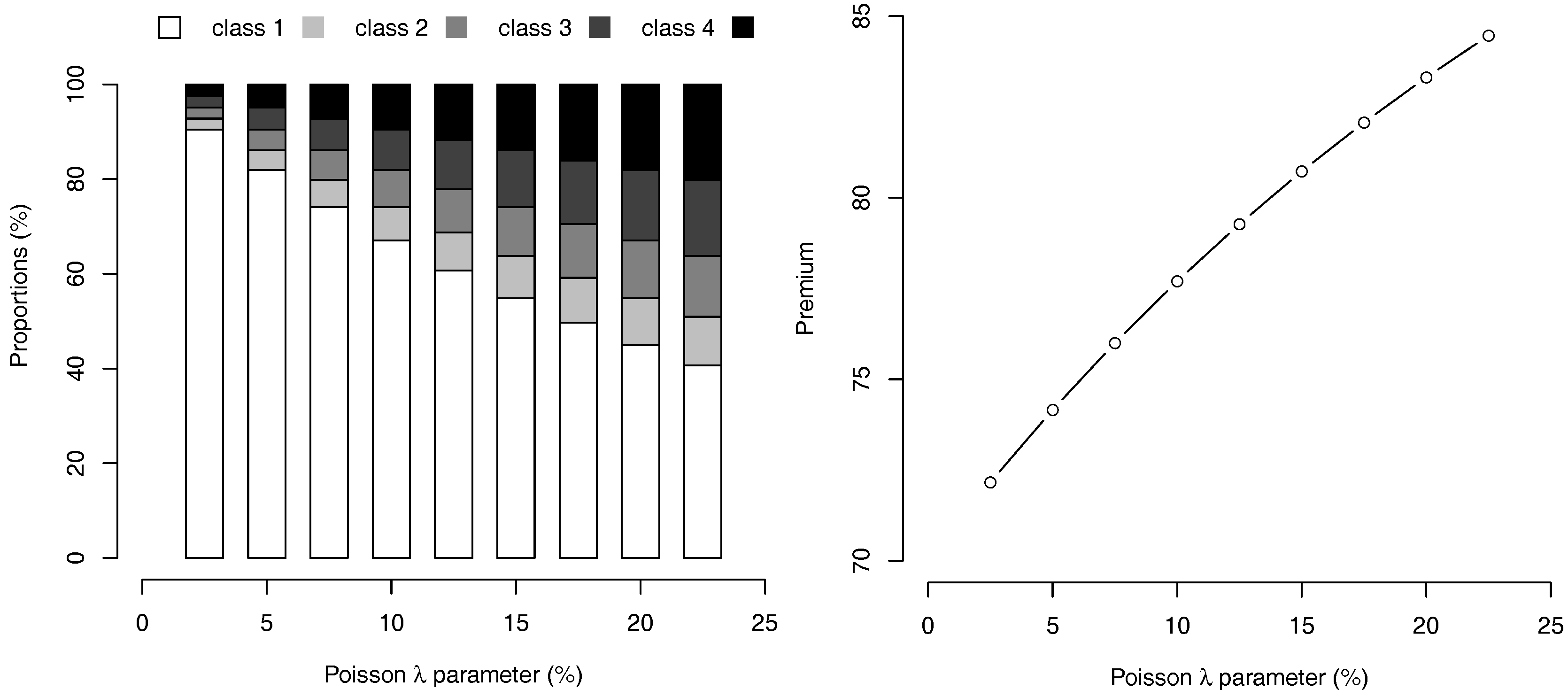
The stationary distribution of the drivers together with the evolution of , for different choices of λ are respectively given in Figure 1. As expected, for higher values of λ, more drivers are present in higher order classes. On the contrary, for , we even have more than 90% of the population in the best class, numbered 1. Similarly, the level of the average stationary premium increases with λ, as shown on Figure 1.
Recall that, in order to enforce the actuarial equilibrium, we chose for numerical applications to pick the average level of loss amount m as
Hence, from λ and , we can derive m, as well as the function G, and apply our numerical algorithm in order to compute the stationary value function associated to each class as well as the optimal reporting strategy, characterized by the implied deductible .
In Table 3, is the discounted value of future premiums under the naive assumption that no accident will occur in the future. is the stationary discounted value of future premium when the optimal strategy is considered. is the implied deductible, and is the probability to declare no loss. Here and future values are discounted with either a discount rate (on the left) or a 2% discount rate (on the right) Deductibles are expressed as percentage of the (annual) premium.
Observe that the deductible is increasing with the class level . A driver with a high premium will be more likely to declare any loss, while a driver with a low premium will try to keep his (good) bonus and will avoid declaring losses on purpose.
The evolution of as a function of the discount rate r, when and for exponentially distributed losses can be visualized on Figure 2. As the interest rate increases, the rational driver will minimize the impact of a reported claim on his future costs, so that he will be eager to declare more accidents, even with smaller levels. Indeed, we observe that the implied deductible is a decreasing function of r, for any class level .
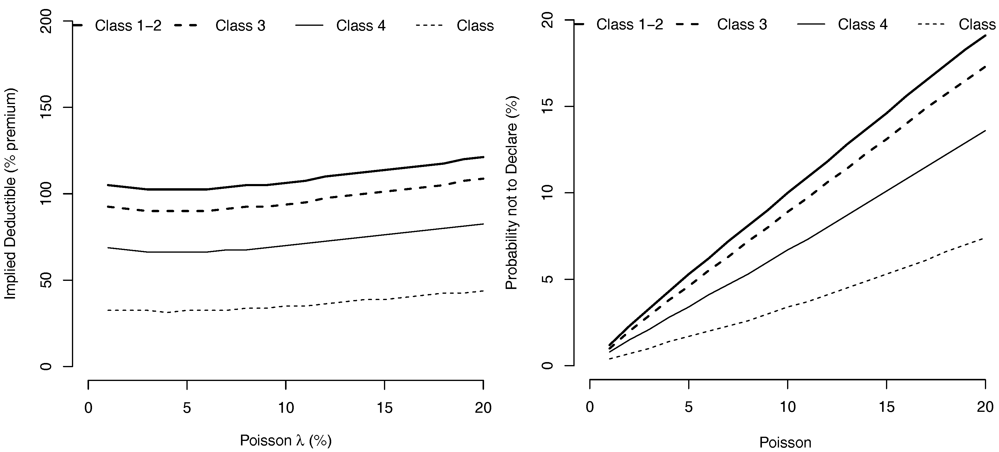
The evolution of as a function of the accident frequency intensity λ, when and loss severity is exponentially distributed can be visualized on Figure 3. Le minimal level for claim reporting slowly increases with the frequency λ of the accident.
Whenever the interest rate r is fixed at and the frequency of accidents is fixed by , Figure 4 shows the evolution of as a function of the coefficient of variation of losses, , for Gamma distributed losses. We observe that high and low variance factors lead to higher deductible levels, meaning that a too small or too large uncertainty on the possible level of loss, provides incitations for the driver not to declare losses of small level.
Finally, as proved in Proposition 3, this optimal claiming strategy yields an updated Markov Chain for bonus classes. More specifically, transition matrix becomes
with a discount rate, and the stationary measure whenever every driver reports his claims is given by
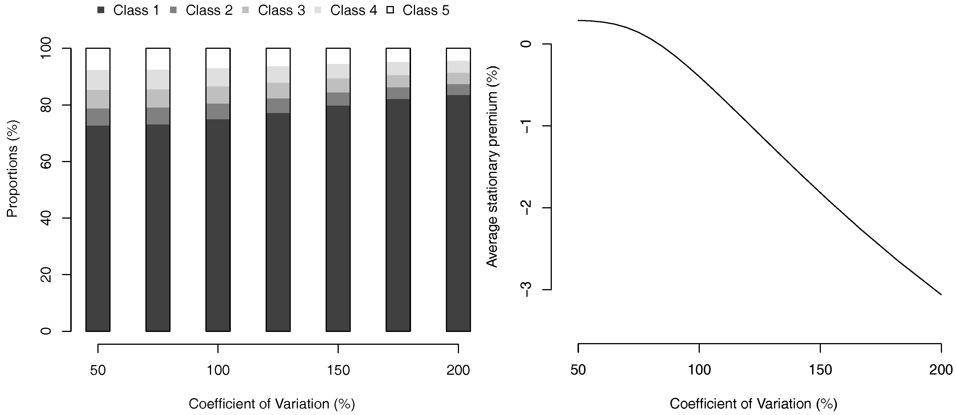
and the stationnary average premium is 75.8. The evolution of the invariante measure and the average premium, as a function of the coefficient of variation (with Gamma losses) can be visualized on Figure 5.
5. Possible Extensions
The model considered so far has on purpose been chosen in its simplest form in order to emphasize the effect of a rationally optimal claim reporting strategy. We now discuss several extension possibilities, which can be encompassed in our framework of study.
5.1. Addition of Deductibles
In order for the model to be more realistic, one should take into account that any driver also has to pay a deductible, whenever a loss is reported, see e.g., Zachs and Levikson (2004). The level of deductible D depends on the current class level s and will be denoted . In such a case, the optimization problem of the agent is replaced by
where the extra term takes into account that one should pay the deductible whenever a loss is reported at time t.
This new formulation gives rise to an optimal strategy which takes the similar form as the one obtained in the no-deductible case:
the only difference relying on the previous modification of the definition of the value function. The characterization for the solution presented in Proposition 1 as well as the approximating algorithm considered in Section 3.3 can be adapted to this setting in a straightforward manner.
5.2. Consideration of Risk Averse Drivers
In the previous setting, the representative driver is considered to be risk neutral, namely he is neither afraid nor eager to take some risk. The rational behavior of the driver may also be represented using a utility function characterizing his choices under uncertainty. In this framework, the new optimization problem of the agent is given by
where U is the chosen risk adverse utility function of the agent. In such a case, once again, the implied deductible is characterized in a similar fashion and only the computation scheme for the value function is modified. Nevertheless, the dynamic programming principal allows us once again to characterize the value function of the agent as the solution to a non linear system of equations. The only difference is that each payment is computed via its utility value instead of solely its monetary one.
5.3. Consideration of Heterogeneous Agents
A tempting extension is to try to incorporate heterogeneity in the driver economic behavior. It is quite classical to consider that drivers may have different probabilities of accident occurrence and severity but less in the actuarial literature to incorporate different economic behavior for agents. In our framework, we could consider a collection of driver types , so that each type x of driver is characterized by its own utility function together with his interest rate . In such a case, a driver of type x will solve the problem
Hence, one can solve these problems separately of any and deduce the corresponding collection of implied deductibles . Then, one can directly compute the corresponding stationary distribution associated to any class . Hence, the average premium should by derivedby aggregating all the driver types and computing
where f represents the density function of the types in the population.
6. Conclusions
We have seen in this paper how hunger for bonus can be incorporated in order to obtain the ‘true’ transition matrix for class levels, not only based on accidents occurrence, but considering the probability to report losses. The dynamic programming problem does not have simple and explicit solutions, but a simple numerical algorithms can be used in order to approximate the solution. We have observed the impact of the hunger bonus in the context of a simplistic Bonus-Malus scheme, but it can be extended easily to more complex ones, as discussed in particular in Section 5. The most difficult remaining task is clearly to obtain the extension to the case where the Bonus-Malus scheme takes into account the number of reported claims within a period. A way to solve it is to assume that the driver waits until the date of renewal, to decide how many losses are reported (and which ones), but if equations can be explicitly written (and solved), this approach is not realistic. This is clearly a difficult task for future research.
We chose in this paper not to consider the ex post or ex-ante moral hazard topics associated to the design of optimal insurance policy. The main reason is that, as long as the Bonus-Malus policy is clearly announced in advance by the insurance company, the rational driver should not have any reason to dissimulate his driving skills, other than the economic one presented above. Finally, our model lacks realism since we assume that any driver is rational, able to take economies decisions as the one described above, and only wishes to make his claim reporting on based on solely economic reasoning, instead of e.g., more ethical ones. A natural extension of for such study would be to consider a chosen distribution of ’rationally reporting’ type of drivers in the population. Finally, the most difficult part is probably that λ is usually unknown by drivers, and this (possibly heterogenous) ambiguity will indice an additional bias.
Acknowledgments
Charpentier received financial support from NSERC and ACTINFO chair. Elie received financial support from ACTINFO chair.
Author Contributions
The three authors contributed equally to this paper.
Conflicts of Interest
The authors declare no conflict of interest.
References
- Abramowitz, Milton, and Irene A. Stegun. 1965. Handbook of Mathematical Functions. Washington: National Bureau of Standards. [Google Scholar]
- Boucher, Jean–Philippe, Michel Denuit, and Montserrat Guillen. 2009. Number of Accidents or Number of Claims? An Approach with Zero—Inflated Poisson Models for Panel Data. Journal of Risk and Insurance 76: 821–46. [Google Scholar] [CrossRef]
- Braun, Michael, Peter S. Fader, Eric T. Bradlow, and Howard Kunreuther. 2006. Modeling the ‘pseudo-deductible’ in insurance claims decisions. Management Science 52: 1258–72. [Google Scholar] [CrossRef]
- Chappell, D., and J. M. Norman. 2003. Optimal, near-optimal and rule-of-thumb claiming rules for a protected bonus vehicle insurance policy. European Journal of Operational Research 41: 151–56. [Google Scholar] [CrossRef]
- Denuit, Michel, Xavier Maréchal, Sandra Pitrebois, and Jean-Francois Walhin. 2007. Actuarial Modelling of Claim Counts: Risk Classification, Credibility and Bonus-Malus Systems. New York: John Wiley & Sons. [Google Scholar]
- De Pril, Nelson. 1979. Optimal claim decisions for a bonus-malus system: A continuous approach. ASTIN Bulletin 10: 215–22. [Google Scholar] [CrossRef]
- Franckx, Edouard. 1960. Théorie du bonus. ASTIN Bulletin 3: 113–22. [Google Scholar]
- Hey, John D. 1985. No Claim Bonus. Geneva Papers on Risks and Insurance 10: 209–228. [Google Scholar] [CrossRef]
- Lemaire, Jean. 1977. La soif du bonus. ASTIN Bulletin 9: 181–90. [Google Scholar] [CrossRef]
- Lemaire, Jean, and Hongmin Zi. 1994. A comparative analysis of 30 bonus-malus systems. ASTIN Bulletin 24: 287–309. [Google Scholar] [CrossRef]
- Lemaire, Jean. 1995a. Automobile Insurance: Actuarial Models. Boston: Kluwer-Nijhoff. [Google Scholar]
- Lemaire, Jean. 1995b. Bonus-Malus Systems in Automobile Insurance. Boston: Kluwer-Nijhoff. [Google Scholar]
- Walhin, Jean-Francois, and Jose Paris. 1999. Using mixed Poisson distributions in connection with Bonus-Malus systems. ASTIN Bulletin 29: 81–99. [Google Scholar] [CrossRef]
- Walhin, Jean-Francois, and Jose Paris. 2000. The true claim amount and frequency distributions within a bonusmalus system. ASTIN Bulletin 30: 391–403. [Google Scholar] [CrossRef]
- Zachs, S., and B. Levikson. 2004. Claiming Strategies and Premium Levels for Bonus Malus Systems. Scandinavian Actuarial Journal 2004: 14–27. [Google Scholar] [CrossRef]
| 1. | Note that we will not address any legal aspects here (in various contries, it might be compulsory to report all accidents), but we focus on incentives modeling issues, and related mathematical aspects. |
| 2. | |
| 3. | This system is no longer in force, and is mainly used for its pedagogical intuition. |
Figure 1.
Invariant probability measure and symptotic premium , as a function of λ, with .

Figure 2.
Value of the Deductibles, (expressed as a percentage of the premium ) and probability not to declare an accident, as a function of the discount rate r.
Figure 2.
Value of the Deductibles, (expressed as a percentage of the premium ) and probability not to declare an accident, as a function of the discount rate r.
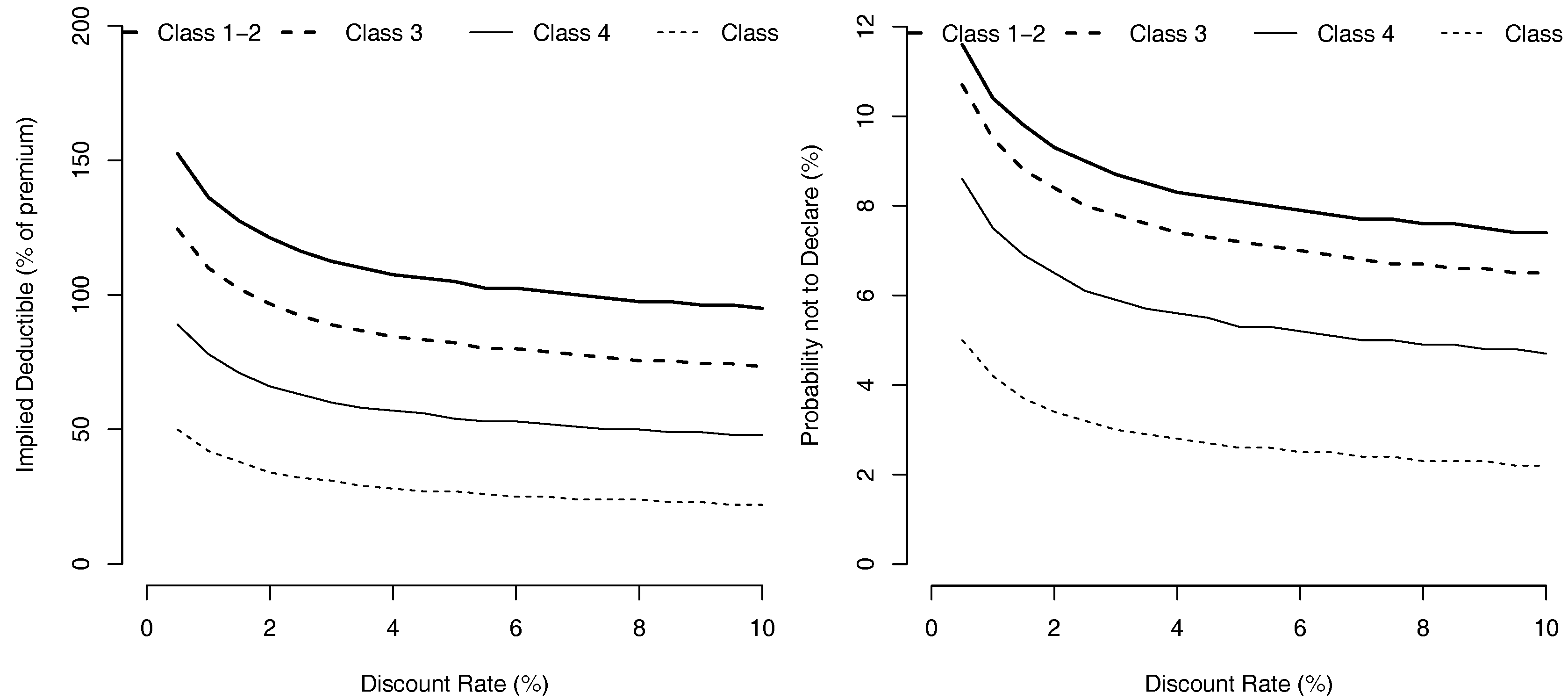
Figure 3.
Value of the Deductibles, (expressed as a percentage of the premium ) and probability not to declare an accident, as a function of annual accidents frequency λ (in %).
Figure 3.
Value of the Deductibles, (expressed as a percentage of the premium ) and probability not to declare an accident, as a function of annual accidents frequency λ (in %).

Figure 4.
Value of the Deductibles, (expressed as a percentage of the premium ) and probability not to declare an accident, as a function of losses coefficient of variation (with a Gamma distribution).
Figure 4.
Value of the Deductibles, (expressed as a percentage of the premium ) and probability not to declare an accident, as a function of losses coefficient of variation (with a Gamma distribution).
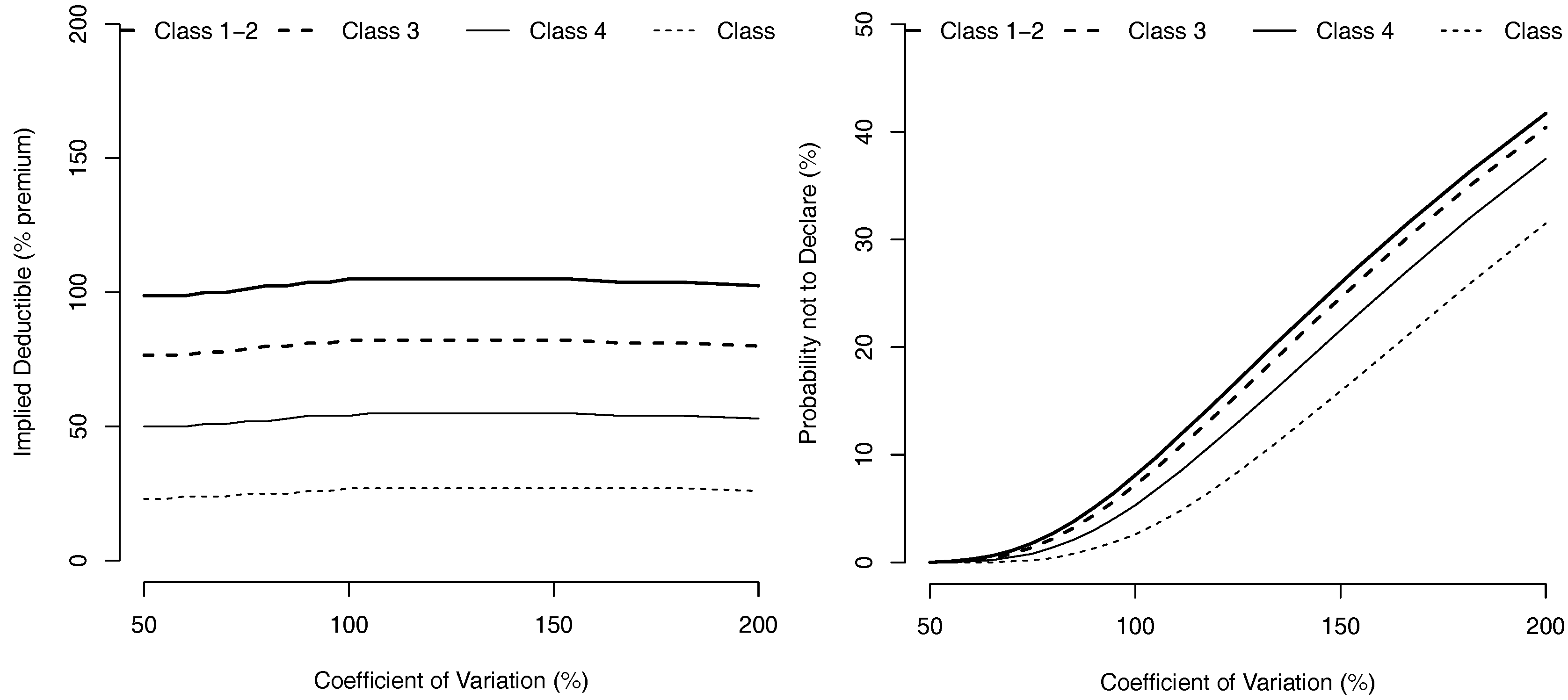
Figure 5.
Proportion in each bonus class (stationary invariante measure) on the left, and stationnary average premium (as a percentage of the classical case where all claims are reported), as a function of losses coefficient of variation (with a Gamma distribution).
Figure 5.
Proportion in each bonus class (stationary invariante measure) on the left, and stationnary average premium (as a percentage of the classical case where all claims are reported), as a function of losses coefficient of variation (with a Gamma distribution).

Table 1.
Transition rules for the 3 class Bonus-Malus system.
| Class | Premium | Claim | No Claim |
|---|---|---|---|
| 3 | 3 | 2 | |
| 2 | 3 | 1 | |
| 1 | 2 | 1 |
Table 2.
Transition rules for the ‘Spanish Bonus-Malus’ scheme.
| Class | Premium | Class after 0 Claim | Class after 1 Claim |
|---|---|---|---|
| 5 | 100 | 4 | 5 |
| 4 | 100 | 3 | 5 |
| 3 | 90 | 2 | 5 |
| 2 | 80 | 1 | 5 |
| 1 | 70 | 1 | 5 |
Table 3.
Impact of the optimal reporting strategy, Exponential losses, and or .
| Class | Premium | ||||||||
|---|---|---|---|---|---|---|---|---|---|
| 1 | 100 | 1481 | 3586 | 1553 | 3128 | 84 ( | 97 ( | 8.1% | 9.3% |
| 2 | 100 | 1455 | 3558 | 1527 | 3094 | 84 ( | 97 () | 8.1% | 9.3% |
| 3 | 90 | 1428 | 3529 | 1499 | 3062 | 74 ( | 87 () | 7.2% | 8.4% |
| 4 | 80 | 1410 | 3510 | 1480 | 3042 | 54 ( | 66 () | 5.3% | 6.5% |
| 5 | 70 | 1400 | 3500 | 1470 | 3032 | 27 ( | 34 () | 2.6% | 3.4% |
© 2017 by the authors. Licensee MDPI, Basel, Switzerland. This article is an open access article distributed under the terms and conditions of the Creative Commons Attribution (CC BY) license (http://creativecommons.org/licenses/by/4.0/).
Share and Cite
MDPI and ACS Style
Charpentier, A.; David, A.; Elie, R. Optimal Claiming Strategies in Bonus Malus Systems and Implied Markov Chains. Risks 2017, 5, 58. https://doi.org/10.3390/risks5040058
AMA Style
Charpentier A, David A, Elie R. Optimal Claiming Strategies in Bonus Malus Systems and Implied Markov Chains. Risks. 2017; 5(4):58. https://doi.org/10.3390/risks5040058
Chicago/Turabian StyleCharpentier, Arthur, Arthur David, and Romuald Elie. 2017. "Optimal Claiming Strategies in Bonus Malus Systems and Implied Markov Chains" Risks 5, no. 4: 58. https://doi.org/10.3390/risks5040058
Note that from the first issue of 2016, this journal uses article numbers instead of page numbers. See further details here.