Stable Weak Approximation at Work in Index-Linked Catastrophe Bond Pricing


1
Faculty of Pure and Applied Mathematics, Hugo Steinhaus Center, Wroclaw University of Science and Technology, 50-370 Wroclaw, Poland
2
Department of Actuarial Science, Faculty of Commerce, University of Cape Town, Rondebosch 7701, Cape Town, South Africa
*
Author to whom correspondence should be addressed.
†
Current address: The African Institute for Financial Markets and Risk Management, University of Cape Town, South Africa.
‡
These authors contributed equally to this work.
Risks 2017, 5(4), 64; https://doi.org/10.3390/risks5040064
Submission received: 28 November 2017
/
Revised: 12 December 2017
/
Accepted: 13 December 2017
/
Published: 16 December 2017
Abstract
:We consider the subject of approximating tail probabilities in the general compound renewal process framework, where severity data are assumed to follow a heavy-tailed law (in that only the first moment is assumed to exist). By using the weak convergence of compound renewal processes to -stable Lévy motion, we derive such weak approximations. Their applicability is then highlighted in the context of an existing, classical, index-linked catastrophe bond pricing model, and in doing so, we specialize these approximations to the case of a compound time-inhomogeneous Poisson process. We emphasize a unique feature of our approximation, in that it only demands finiteness of the first moment of the aggregate loss processes. Finally, a numerical illustration is presented. The behavior of our approximations is compared to both Monte Carlo simulations and first-order single risk loss process approximations and compares favorably.
1. Introduction
One of the most important types of insurance-linked securities has been the catastrophe (CAT) bond, which, in a broad sense, provides ex-ante capital to the issuer in the case of a pre-defined catastrophe-related event happening. However, despite various theories on how to value such bonds, their pricing still remains difficult because of the jump processes and heavy-tailed distributional assumptions, which most often underpin such theories. In this paper, we focus on how, in the context of certain traditional CAT bond pricing models, one can simplify and quicken CAT bond pricing by using approximations to their assumed underlying processes.
We now present a brief overview of CAT bonds. CAT bonds have been loosely classified into three main types: indemnity-linked, index-linked and parametric (see Cummins and Weiss (2009)). Such classification is based on the “trigger” of the bond, that is the event (or set or even sequence thereof) that causes the bond to release the capital to the issuer. In this research, we, however, focus on index-linked CAT bonds, which, according to the Artemis deal directory, have the second-largest issuance outstanding in the 2016 CAT bond market (Artemis 2016).
The pricing of CAT bonds is complex. This is mainly because these securities, and other insurance-related derivatives as well, will have a process with jumps as an important modeling component (such as, for example, a compound Poisson process or shot-noise process (see Dassios and Jang (2003) and Schmidt (2014) for an application of these processes to catastrophe derivatives), and therefore, unique prices based on arbitrage-free pricing techniques in general do not exist (Chang and Chang 2017; Embrechts 2000; Embrechts and Meister 1997; Lee and Yu 2002). Therefore, it seems clear as to why there have been discussions around a number of methods for pricing CAT bonds. Five differing theoretical frameworks have been postulated in the literature thus far (Braun 2011; Galeotti et al. 2013). Firstly, standard actuarial pricing methodologies have been applied to CAT bonds by Lane and Mahul (2008) and Bodoff and Gan (2009). Secondly, an econometric CAT bond pricing model, based on observable catastrophe-related quantities, was proposed by Braun (2016), for pricing in the primary market. Thirdly, utility-based approaches have been proposed by Cox and Pedersen (2000); Egami and Young (2008); Reshetar (2008) and Dieckmann (2010) for numerous types of CAT bonds. Fourthly, preference-free no-arbitrage frameworks have been proposed to price CAT bonds, and these frameworks have, in fact, been more traditional and more frequently used. Baryshnikov et al. (1998) undertook the first attempt to price catastrophe bonds within a no-arbitrage framework. They argued that the risk-neutral and real-world probability measures would coincide. As a consequence, further no-arbitrage pricing developments arose in Burnecki and Kukla (2003); Härdle and Cabrera (2010); Jarrow (2010); Lee and Yu (2002); Loubergé et al. (1999); Ma and Ma (2013); Nowak and Romaniuk (2013); Vaugirard (2003a 2003b 2004); and recently in Jaimungal and Chong (2014). Finally, pricing concerns surrounding incomplete markets, and non-unique measures can be overcome by a judicious choice of change in measure, such as the Esscher transform (see Gerber and Shiu (1996)). Another approach, similar to this, is the Wang transform introduced by Wang (2000).
Given the pervasiveness of the usage of aggregate loss processes (ALPs), such as compound Poisson processes, in most of the CAT bond pricing frameworks, it is important to mention the difficulty in explicitly evaluating functionals of the ALP. It is, however, possible to approximate the exact cumulative distribution function of the compound Poisson process using either Fourier transforms, numerical simulation techniques or approximation methods. So far, the literature on CAT bonds’ attention appears to be mainly on numerical simulation techniques, such as Monte Carlo simulation. Monte Carlo simulation and quasi-Monte Carlo simulation have been applied to numerically evaluating the pricing formulae (Burnecki et al. 2005; Nowak and Romaniuk 2013). However, Monte Carlo has to be used with caution, since one is working with the simulation of heavy-tailed data (Burnecki and Giuricich 2017), and therefore, more sophisticated techniques such as importance sampling need to be used.
Approximation methods for evaluating cumulative distribution functions of the compound Poisson processes have been used (Ma and Ma 2013). Such approximations of the compound Poisson random variable include the normal approximation, the normal power approximation, the Edgeworth approximation (Beard 2013; Pentikäinen 1977), the gamma approximation (Seal 1977; Sundt 1982), the inverse-Gaussian approximation (Chaubey et al. 1998) and the Esscher approximation (Esscher 1932). For a comprehensive treatment of the comparison of their errors, see Seri and Choirat (2015). A problem noticed with the usage of such approximations is that their applicability is not always possible in the cases when the underlying severity distributions have only finite first moments.
Now in light of the aforementioned, it seems that despite attempts to numerically evaluate the ALP-based pricing formulae for CAT bonds, no simple, approximate pricing formulae have been derived in the case of very heavy-tailed distributional assumptions. Therefore, we endeavor to fill this gap in the literature.
In this paper, we consider the class of -stable distributions and associated motions. To tie the notion of -stable Lévy motion to catastrophe modeling and CAT bond pricing, we present an approximation, of the ALP assumed to underlie CAT bonds, to -stable Lévy motion by invoking the concept of weak convergence of one process to another. This approximation technique has its roots in ruin theory (see Grandell (2012), Furrer et al. (1997), Burnecki (2000) and Michna (2005)) and considers loss severity distributions belonging to the domain of attraction of -stable laws. We highlight that this approximation explicitly accounts for (and indeed accommodates for) the heavy-tailed nature of the losses (and loss processes) giving rise to CAT bond price behavior.
With our goal in mind, Section 2 begins by providing the necessary theoretical framework to construct the weak approximations to -stable Lévy motion. In Section 3, we present our results and derivations on the convergence of the ALPs to -stable Lévy motion. Section 4 applies the general results of Section 3 to compound Poisson processes. Based on specific examples of loss severity distributions for the ALP (taking the form of a compound Poisson process), we then present closed-form approximations for index-linked CAT bond prices. Section 5 introduces the existing index-linked CAT bond pricing model we use, and Section 6 shows our approximations at work in this practical setting. We then go on to compare our approximations to standard Monte Carlo simulation exercises for simulating the ALP and also first-order single risk loss process approximations. Moreover, in this section, we provide some guidance on how to test if our approximations are applicable to the situations considered. Section 7 concludes.
2. Theoretical Framework: Weak Convergence of the Aggregate Loss Process to -Stable Lévy Motion
We begin by contextualizing what we have in mind for the mathematical model for the ALP. We firstly consider a renewal process, as given by Definition 1.
Definition 1.
Now, we simply assume that the renewal process governs the frequency component in the ALP and that successive losses form a sequence of iid random variables only with . Therefore, our ALP takes the form:
which is, in essence, a compound renewal process. The remainder of this section will be devoted to discussing the definitions of -stable distributions and processes, some assumptions for our paper and the idea of weak convergence.
2.1. -Stable Distributions and -Stable Lévy Motion
The applicability of Gaussian distributions and processes in stochastic modeling has been extensively studied. However, analyses of insurance, as well as financial data often points to the existence of heavy tails (see, for example, Embrechts et al. (2013) and the recent work by Calderín-Ojeda et al. (2017)), calling the use of Gaussian distributions into question. The more general class of stable distributions can account for such a heavy-tailed feature in the data.
The theory regarding univariate stable distributions was developed in the early 1900s and is covered in detail in the books of Janicki and Weron (1994), Samorodnitsky and Taqqu (1994) and the forthcoming book of Nolan (2015). Despite there being a few ways to define it, we define a stable random variable in terms of its characteristic function to explicitly emphasize its associated parameters.
Definition 2.
(Samorodnitsky and Taqqu (1994) and Janicki and Weron (1994)) A random variable X is said to have a stable distribution, written , if there are parameters (the index of stability), (the skewness parameter), (the scale parameter) and (the shift) such that its characteristic function has the following form:
Furthermore,
The parameters and ν are unique and β is irrelevant when .
The notation indicates that the random variable X has a stable distribution with four parameters and . Note that densities for stable random variables expressed in terms of elementary functions only exist in the cases when (the normal distribution), (the Cauchy distribution) and (the Lévy distribution). Moreover, bear in mind that the rate of decay in the stable distribution mostly depends on the parameter . We now define what is meant by an -stable Lévy motion.
Definition 3.
(Samorodnitsky and Taqqu (1994) and Janicki and Weron (1994)) A stochastic process is called an α-stable Lévy motion if:
- (i)
- a.s.;
- (ii)
- has independent increments;
- (iii)
- for any , for some and for .
Observe that the process introduced in Definition 3 has stationary increments, and it is Brownian motion when . We now present some useful properties, which will be relevant to our expositions in Section 3, Section 4 and Section 6.
- Property 1: existence of moments. If , and , then and if , then
- Property 2: tail probability estimation. If and , then:where:
- Property 3: self-similarity. -stable Lévy motions are -self-similar. That is, for all and have the same finite-dimensional distributions.
We also point out that Property 2 will feature prominently in our work: we will apply it in approximating probabilities for -stable random variables. We do, however, highlight that there are other means to approximate such random variables and processes; see Kohatsu-Higa and Tankov (2010), for example.
Before we present the idea of weak convergence, we introduce an important assumption underlying our work. We assume that our sequence of iid loss random variables underlying the ALP (see Equation (1)), each with finite mean , satisfies:
where denotes convergence in distribution, (where L is slowly varying at infinity) and is an -stable random variable with . Based on this assumption, we say that our ’s are in the domain of attraction of an -stable random variable , the former random variable only having a finite first moment.
2.2. Weak Convergence of the Aggregate Loss Process
Let denote the space of all real-valued Càdlàg functions on endowed with the Skorokhod topology. Then, is a separable and complete metric space, where is the Skorokhod metric as defined in Skorokhod (1957). See Lindvall (1973) for further details.
Definition 4.
(Billingsley (2013)) A sequence of stochastic processes is said to converge weakly in to a stochastic process X if for every bounded functional f on , it follows that:
When a sequence of stochastic processes satisfies Equation (3), we will write .
We now turn to showing that in general, the ALPs we consider do converge to a stable Lévy motion, and we moreover apply the results of Furrer et al. (1997) and Michna (2005) to ALPs. For our sequence of iid losses satisfying Equation (2) and , a sequence of renewal processes, if:
in probability in , for and for a positive constant , then:
where is an -stable Lévy motion (Furrer et al. 1997). Observe that if L is a constant, say d, then we may rewrite Equation (5) as:
Note that in light of Definition 1, we can set in Equations (4) to (6) since is a renewal process. Now, the relationship in Equation (6) is a central idea to our application of the weak convergence to an -stable Lévy motion. However, Equation (6) provides no guidance on how to explicitly find the constant d and the explicit value of . We now present a less general version of Nolan (2015)’s generalized central limit theorem, which helps us find d. Suppose that is an iid sequence of random variables each having common distribution function F firstly with , secondly exhibiting tail probabilities that satisfy and for and thirdly with . Then:
The sequences and , as well as the the constant , are given by:
Notice that the sequence is crucial in finding d. That is, , which depends on the distributional form of the ’s. Moreover, it is clear that given the severity distribution, will be equal to a function of its parameters.
Some comments on the applicability of Equation (6) now follow. In selecting ALPs to model the underlying catastrophe risk inherent in CAT bonds, often heavy-tailed severity distributions are selected. Therefore, in the forthcoming sections of this paper, we shall restrict ourselves to the application of the generalized central limit theorem to heavy-tailed distributions assumed to belong to the domain of attraction of an -stable distribution with . Thus, the mean of these distributions is finite; however, the higher-order moments need not be finite. We also point out that while classical Brownian motion approximations to ALPs (see Embrechts et al. (2013) and also Grandell (2012)) require light-tailed distributions, this assumption can be relaxed in the more general context of -stable Lévy motion approximations.
3. Weak Approximation of Tail Probabilities of Compound Renewal Processes
Index-linked CAT bond pricing often requires the computation of probabilities such as , where D is some positive constant. An example of this is in the case of an index-linked CAT bond that has an associated threshold level (say D). That is, should total accumulated losses (from a pre-specified source) over a period of time exceed this threshold level, the CAT bond triggers and releases some pre-defined amount of capital to the issuer. Therefore, it is of interest to obtain an approximation to the aforementioned probability. In their index-linked CAT bond pricing framework, Ma and Ma (2013) considered a mixed approximation to this probability. However, their approximation, which relies on higher-order moments and cumulants of the loss process, was not always valid since many of their fitted severity distributions did not possess finite second-order (and higher) moments and cumulants. We now consider how to overcome this problem and therefore approximate index-linked CAT bond prices under heavy-tailed distributional assumptions.
We begin by emphasizing that we consider the case when the severity distribution lies in the domain of attraction of an -stable distribution with , which implies that only the first moment is finite. We now present a theorem that allows us to weakly approximate the probability . The basic idea is to consider the compound renewal process over the time period and replace it by a suitable -stable Lévy motion and, within this sphere, apply known results on tail probability estimation to find a closed-form expression for the required probability. Note the notation used in Theorem 1: if and are two functions, by , we mean that .
Theorem 1.
Let be a renewal process as defined in Definition 1, and suppose that for each of the ’s. Then, let the constant D be represented as , where . Then, we have, for T a positive constant,
where , β is the skewness parameter of the limiting α-stable distribution and where d is a constant that depends on the distributional form of the ’s.
Proof.
For T a positive constant, define the sequence of random variables in as follows:
By a time transformation on N, we can specify that:
where is a renewal process with unit intensity and . By Equation (4), the second term converges to zero in probability, and by Equation (5), the first term converges weakly to , both as . The remaining terms converge to . As a consequence, converges weakly to . Since the random variable is continuous:
By the self-similarity property of (Property 3), it can be shown that:
Finally, the statement follows by invoking the tail probability estimation of an -stable random variable (Property 2). ☐
4. Application to Compound Poisson Processes and Selected Severity Distributions
In Section 2 and Section 3, we assumed that the ALP took the form of a compound renewal process. The ALPs that index-linked CAT bond pricing formulae are most often based on are compound Poisson processes (which are special cases of compound renewal processes), and in this section, we suppose that is indeed a compound Poisson process. Moreover, in the context of index-linked CAT bond pricing, such ALPs often assume a parametric form for the underlying severity distribution component.
4.1. Underlying Parametric Severity Distributions Considered
We consider three types of severity distributions, assumed to belong to the domain of attraction of an -stable random variable (on the basis of their parameters). Their parameterizations are shown in Table 1. Notice that the modified generalized extreme value distribution considered here is the classical generalized extreme value distribution with location parameter set equal to . This action is taken so that this distribution is defined on the positive reals, a support that is consistent with the modeling of insurance losses.
4.2. Compound Poisson Processes
We now apply Theorem 1 to both time-homogeneous and time-inhomogeneous Poisson processes, each of which can underlie the considered ALP, . The following two corollaries specify the results for calculating the required probabilities .
Corollary 1.
Let be a time-homogeneous Poisson process with constant intensity λ, and suppose that for each of the ’s. Let D be represented as , where . Then, for a positive constant T
Proof.
By setting , the statement is an immediate consequence of Theorem 1. ☐
Corollary 2.
Let be a time-inhomogeneous Poisson process with a time-dependent intensity , and suppose that for each of the ’s. Let D be represented as , where and . Then, for a positive constant T,
Proof.
Let us define a time-homogeneous Poisson process with constant intensity . This process at time T has the same distribution as the process . Hence, by Corollary 1, we obtain the thesis. ☐
Observe that Corollaries 1 and 2 are applicable when the follow a Burr, generalized Pareto (GP) or modified generalized extreme value (MGEV) distribution belonging to the domain of attraction of an -stable random variable; that is, the distributions satisfy Equation (2). In order to apply the corollaries to the Burr, GP and MGEV distributions, it is necessary to find the associated index of stability , as well as associated skewness parameter for each distribution and then find d. Under the assumption that , this was all done by applying the generalized central limit theorem from Section 2.2, and Table 2 provides the relevant values. Notice that d is the same in the case of both the GP and MGEV distributions.
5. Classical Catastrophe Bond Pricing
In this section, we briefly present the index-linked CAT bond pricing model used to illustrate the usefulness of the weak approximations derived in Section 4. We use the preference-free index-linked CAT bond pricing framework of Ma and Ma (2013), with the assumption of a constant interest rate. Importantly, we motivate the use of their pricing framework by the fact that we extend it to circumstances where the underlying distributions are assumed to be heavy-tailed. We briefly recap their framework here and point out that the approximation formulae derived in Section 3—namely Equations (8) and (9)—are highly applicable in the context of their model.
Before presenting the pricing formulae, take note of the less general model setting in which we are now operating. We assume that the ALP, , is a compound time-inhomogeneous Poisson process with frequency component having intensity function and the severity distribution component assumed to be as in Section 4. However, we do point out that the usage of our approximation formulae (namely Equation (7)) is not limited to the case where is a compound Poisson process. They can also be used in the more general case where is a compound renewal process, and the classical index-linked catastrophe bond pricing framework we use can potentially accommodate for this generalization.
Crucially, it is assumed for the purpose of this exercise that and are independent. Moreover, independence between financial market risk variables (such as interest rates) and catastrophe risk variables (such as insurance loss processes) is assumed.
5.1. General Pricing Rule
Let be a probability space. In an arbitrage-free financial market, the time-t discounted value of a contingent claim , , at time , under the real-world probability measure can be written as:
where denotes the expectation under the real-world probability measure, r is the constant interest rate over the period and is the associated filtration up until time t.
Notice that the expectation is taken under the real-world probability measure . This is because in the classical pricing framework, under the risk-neutral probability measure, distributions and stochastic processes employed to price CAT bonds have the same distributional characteristics as under the real-world probability measure. Ma and Ma (2013) derived Equation (10) under a risk-neutral measure using the diversification arguments of Merton (1976). However, due to their assumption that catastrophe risk variables are measure independent, Equation (10) is consequently reflected under . It must be noted that similar arguments, based on the work of (Merton (1976), were also used recently in the context of catastrophe reinsurance contracts by Chang and Chang (2017).
5.2. Application to Index-Linked Catastrophe Bond Payoffs
We now consider two payoff structures for CAT bonds and a valuation time of . The first we consider is an index-linked zero-coupon (ZC) CAT bond, having maturity time . The structure of the payoff, , of the ZC CAT bond is given by:
where D is the bond’s contractually-specified threshold level triggering its payoff; and () expresses the constant recovery rate on the bond should the aggregate losses from the index exceed D at time T.
Therefore, the price at time 0, , of the ZC CAT bond is given by:
In the case of an index-linked coupon-paying (CP) CAT bond, having maturity time , constant coupon rate and coupon-paying dates () as measured from the valuation date, the structure we assume for the bond is as follows. For each coupon paying date , the payoff per unit nominal is:
where is defined as in the ZC CAT bond case and is the index-linked CP CAT bond’s pre-defined threshold level. Observe that the coupon-paying bond has both its coupons and redemption amount written down by should the threshold be exceeded. At Time 0, the price, , of the index-linked CP CAT bond having maturity time is given by:
6. Numerical Illustration
6.1. Overview and Background
In order to appreciate the behavior of our weak approximation in the context of our chosen index-linked CAT bond pricing model, we give a numerical illustration. Moreover, we assess the behavior of such an approximation on the basis of heavy-tailed distributions commonly used in the literature on index-linked CAT bond pricing.
We emphasize that the weak approximations for the compound Poisson process derived in Corollaries 1 and 2 can be directly inserted into the classical CAT bond pricing formulae given by Equations (12) and (14), assuming that the constants D and are indeed the threshold levels of the index-linked CAT bonds. We do so and numerically compare our simple approximation firstly to Monte Carlo (MC) estimated prices (see Burnecki and Giuricich (2017) for an outline of the procedure) and secondly to a simple first-order single risk loss process (FSRLP) approximation. The idea behind the FSRLP is that if we assume the severity, , is sub-exponential and that the number of losses is Poisson distributed over the time interval of interest, then in our case, can be approximated by (Daley et al. 2007; Peters and Shevchenko 2015; Stam 1973). We re-emphasize that the aim of our work in this section is two-fold. Firstly, it is to compare the performance of our weak approximation against MC simulation (which, in the limit, will give the exact price under the pricing model used). Secondly, it is also a first foray into the comparison the performance of our weak approximation to that of the FSRLP approximation, each relative to MC simulation. We do, however, not attempt to conclude, in general, on the relative superiority or inferiority of our weak approximation to the FSRLP approximation.
For the purposes of this illustration, we consider the ALP fitted by Burnecki and Giuricich (2017), i.e., a compound time-inhomogeneous Poisson process with a time-dependent intensity. That is, the fitted intensity function is:
We use Equation (15) in conjunction with each of the considered severity distributions. For the severity distributions considered in Table 1, we adopt the parameters fitted by the conditional complete-data (CCD) approach (Burnecki and Giuricich 2017). We stress that these parameters are based on Property Claims Services (PCS) insured loss data—data that are indeed left-truncated—so we select the CCD-fitted parameters in order to account for the left-truncation feature. These parameters are provided in Table 3.
For the fitted GP, Burr and MGEV distributions in Table 3, we point out that their associated ’s are all within the range , and as a consequence, all belong to the domain of attraction of an -stable distribution with . Therefore, all distributions only have finite first moments. However, notice that for the MGEV distribution, the power law exponent is so close to one that it will produce numerical errors in simulation. As a consequence, we omit the MGEV distribution from further analysis.
6.2. Is (or ) Large Enough?
In any attempt to apply Theorem 1 to the PCS data, an immediate question arises. Is the fitted intensity , be it constant or (as in Equation (15)) time-dependent, satisfactorily large enough? Note that for the PCS dataset we study, the constant intensity is approximately 27.91 events per year, while the time-dependent fitted intensity function begins at 24.93. We checked this issue by analyzing if for the fitted , is sufficiently close to for each of the Burr and GP severity distributions for fixed threshold levels. We estimated the former probability via 100,000 Monte Carlo simulations.
For our data, as tended to infinity, converged to as expected. At , the two probabilities appeared to be sufficiently close to one another for both severity distributions: lay within a three standard deviation error bound for for each distribution. However, the approximation appeared to be fairly accurate for all values of in excess of 30 and also for low values of less than 10.
On balance, and under the assumption that the PCS dataset follows a compound Poisson process, the use of Theorem 1 does seem suitable. However, we do caution that its usage does not lead to an exact result, but rather a suitable approximation. We end by emphasizing that if Theorem 1 is to be applied to other datasets, it must be checked that is large enough in order to apply it.
6.3. Numerical Results
In Table 4 and Table 5, we present some numerical values, for illustrative purposes, in the case of pricing index-linked ZC and CP CAT bonds (at Time 0), respectively. The CAT bond threshold level is assumed to be in line with that used by Ma and Ma (2013) (that is million), and we set years, and in Equations (12) and (14). After approximating prices via our weak approximation and the FSRLP approximation and estimating prices by MC simulation, we calculate relative errors. The relative errors of the weak approximation prices () to MC simulation prices () and secondly of the FSRLP approximated prices () to MC simulation prices are calculated by and , respectively. Note that we used 100,000 MC simulations. Pricing surfaces (based on weak approximations) and relative error comparisons (to MC simulation) are shown in the Appendix A and Appendix B. More precise relative error comparisons, for year, for each severity distribution (Burr and GP) are illustrated in Appendix C.
The behavior of our approximation appears to vary according to the underlying severity distributional assumption. It appears that within the realm of our numerical calculations, the closer to unity the power law exponent of the severity distribution, the less well-behaved the approximation (compared to MC estimation and the FSRLP approximation) for low threshold levels and times to maturity. This was indeed the case with the MGEV distribution, hence its omission
We now report on the cases of the fitted GP and Burr distributions, which both have associated ’s further away from unity (1.099 and 1.370, respectively). Upon inspection of Table 4 and Table 5, as well as Figure A1 and Figure A2, it seems clear that for high threshold levels and long terms to maturity, the weakly approximated and the MC-estimated CAT bond prices are similar. This is especially true as the threshold levels D and tend to infinity. We also note that the weakly approximated prices, in both the context of the index-linked ZC and the CP CAT bonds, are similar to not only the MC-estimated prices, but also the prices based on the FSRLP approximation, an approximation that is known to work quite well in the context of compound Poisson process tail probability estimation. In fact, the weakly approximated prices are, mostly, closer to the MC estimated prices in absolute relative error as the threshold level approaches infinity than the FSRLP approximated prices (particularly in the case of the ZC bonds). This may be the case because our approximation is indeed useful in the case of heavy-tailed data. However, Figure A3 shows that this behavior is not always the case for lower threshold levels (for all severity distributions): for index-linked ZC CAT bonds, the weak approximation is better in relative error, while for index-linked CP CAT bonds, the FSRLP is better in relative error. Given that the approximation is used more often in the index-linked CP CAT bond pricing formula (see Equation (14)) and also at different durations in time, we posit that the weak approximation is poorer at shorter time durations than longer ones, for lower threshold levels. This makes sense from the point-of-view that threshold exceedance probabilities are vanishingly small for shorter and shorter durations. However, the FSRLP performed better at shorter durations for lower threshold levels (i.e., lower than ); further numerical analysis into this indeed revealed it was the case.
We do remark on the following two challenges as regards our weak approximation usage in CAT bond pricing. Firstly, we noticed in our numerical analysis that Theorem 1 led to the calculation of probabilities in excess of one. We omit these price calculations from the pricing surfaces in Figure A1 and Figure A2, hence their jagged look. Since we are invoking a weak approximation to probabilities (see Theorem 1, as well as Corollaries 1 and 2) that are not restricted to the interval , we can expect there to be probabilities in excess of one, so this limits the usage of the weak approximation especially for index-linked CAT bonds with low threshold levels and/or short terms to maturity. The second drawback concerns the following: the approximation does not lead to real solutions for small threshold levels D: in fact, for small threshold levels, the approximation is not valid since we cannot find a positive value for M (since in Theorem 1, M depends on D, for fixed D). However, this is as expected (for both distributional assumptions) since the approximation result in Equation (7) is for when , and indeed, such small threshold levels are not evident in index-linked CAT bond pricing practice.
7. Conclusions
In this paper, we considered index-linked ZC and CP CAT bonds under the pricing framework of Ma and Ma (2013). As the pricing formulae obtained under this framework were not in closed-form, we invoked a weak approximation of the ALP (assumed to be a compound renewal process) to -stable Lévy motion. Thereafter, we presented Theorem 1, which allowed one to weakly approximate tail probabilities pertaining to this type of ALP, and then specialized the approximation to the case of a time-inhomogeneous compound Poisson process. The unique, contributing feature of our approximation was that it can be used in the case of heavy-tailed distributions (in particular for when only the first moment is finite) and as a useful check for existing approximations such as the FSRLP approximation. Since such probabilities are essential in computing CAT bond prices, we emphasize the applicability of our weak approximation in obtaining a way to indeed approximate such prices.
Our weak approximation has also other beneficial applications in the insurance sector. Our simple, fast and relatively accurate (compared to Monte Carlo simulation and FSRLP approximations) weak approximation may be applied in the context of other CAT bond pricing models such as in computing attachment probabilities for use in the Lane Financial model of Lane (2003), especially when the losses follow heavy-tailed distributional assumptions. Moreover, our approximation can be applied in approximating loss-exceedance probabilities for reinsurance portfolios and also in estimating premiums for catastrophe excess-of-loss reinsurance contracts. Finally, applications, within the sphere of quickly estimating exceedance probabilities for operational risk purposes, are also possible.
We close by briefly recapitulating some of the limitations and general advantages of our weak approximation to the ALP, noticed in the context of Burr and GP-distributed severity components. In this research, we pointed out three limitations. Firstly, we highlighted that the application of our approximation needs to be assessed on a case-by-case basis. It remains to be checked (by the user of our approximation) that the fitted intensity (or its integration) is large enough for our approximation to be applied. Secondly, our weak approximation did not perform well relative to MC estimation and the FSRLP approximations for shorter time horizons. Thirdly, in the extreme cases, our weak approximation did lead to probabilities in excess of one, so this needs to be checked for. However, we posit that our weak approximation does still have merit. Our weak approximation was found to be simple and computationally inexpensive to implement. Moreover, our weak approximation performed similarly to the more traditional approaches of MC estimation and the FSRLP approximation in most situations, but for longer time horizons, our approximation fared better, in the context of all our numerical illustrations. However, most importantly, we stress our weak approximation’s applicability in situations where data follows a heavy-tailed law; this is, ultimately, because our weak approximations only demand finiteness of the first moment of the loss severity distribution.
Acknowledgments
We gratefully acknowledge Peter Ouwehand, David Taylor, Zbigniew Palmowski, as well as Melusi Mavuso for their valuable comments and suggestions. We also remain indebted to two anonymous Risks referees for their insightful and useful remarks, which all helped to improve the original draft of the paper.
Author Contributions
Each author contributed equally to this work.
Conflicts of Interest
The authors declare no conflict of interest.
Appendix A
Figure A1.
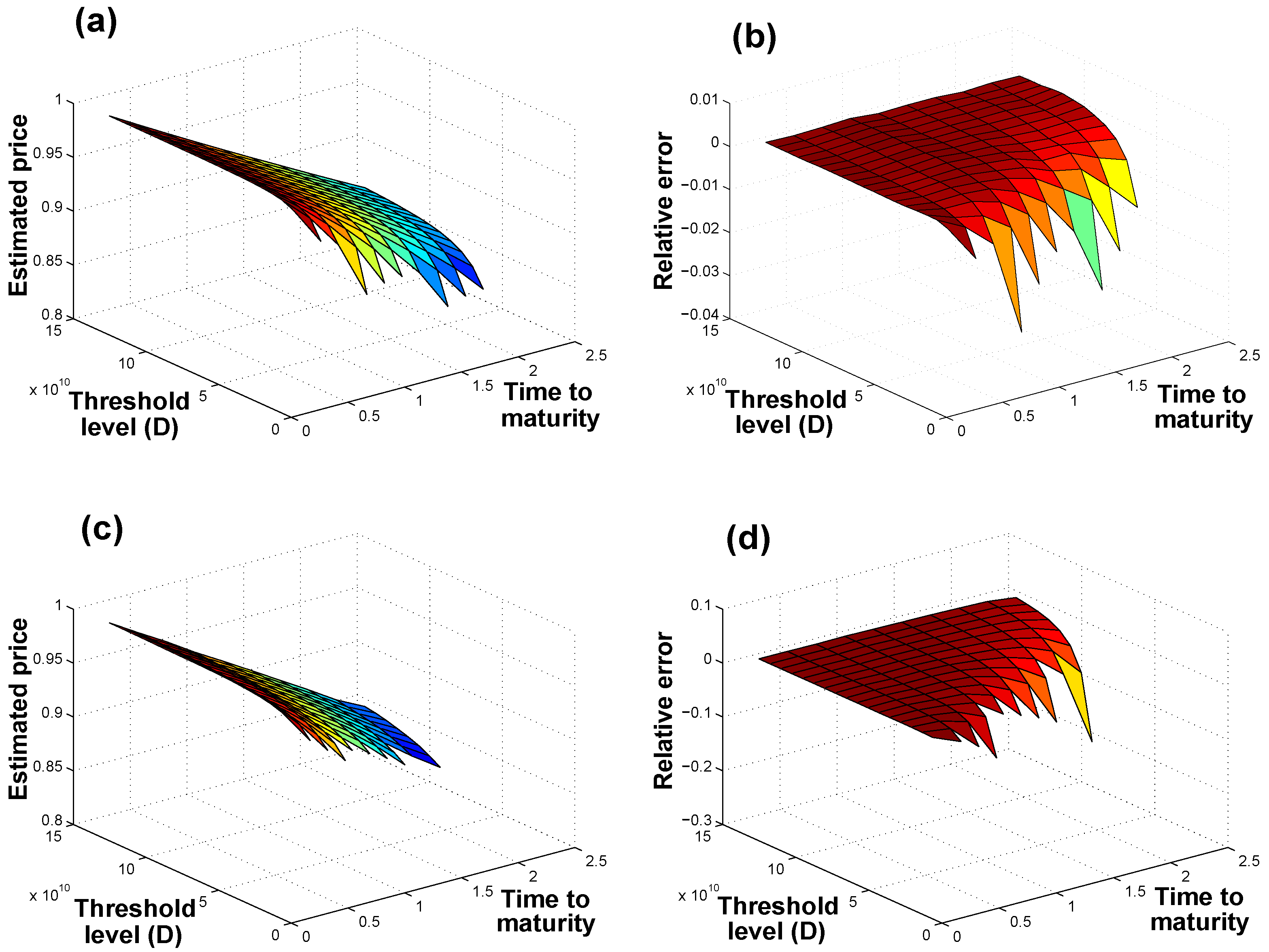
Pricing surfaces, obtained by using the stable weak approximations, for index-linked ZC CAT bonds under the assumption of: (a) GP distributed losses (and the relative error to MC estimation in (b)); and (c) Burr distributed losses (and the relative error to MC estimation in (d)). Note the omission of points where the weak approximations were non-applicable, hence affording the figures their jagged look.
Figure A1.
Pricing surfaces, obtained by using the stable weak approximations, for index-linked ZC CAT bonds under the assumption of: (a) GP distributed losses (and the relative error to MC estimation in (b)); and (c) Burr distributed losses (and the relative error to MC estimation in (d)). Note the omission of points where the weak approximations were non-applicable, hence affording the figures their jagged look.
Appendix B
Figure A2.
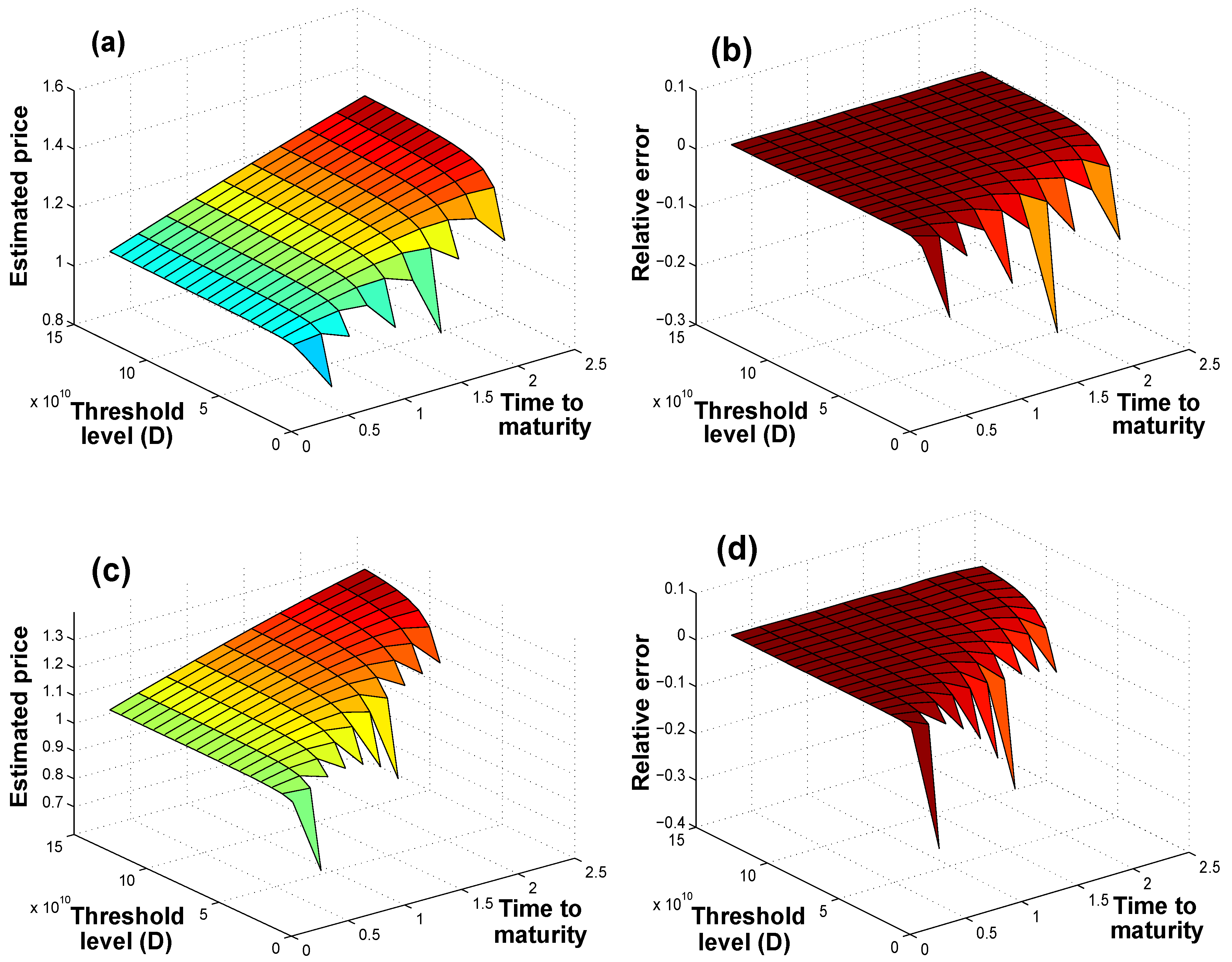
Pricing surfaces, obtained by using the stable weak approximations, for index-linked CP CAT bonds under the assumption of: (a) GP distributed losses (and the relative error to MC estimation in (b)); and (c) Burr distributed losses (and the relative error to MC estimation in (d)). Note the omission of points where the weak approximations were non-applicable, hence affording the figures their jagged look.
Figure A2.
Pricing surfaces, obtained by using the stable weak approximations, for index-linked CP CAT bonds under the assumption of: (a) GP distributed losses (and the relative error to MC estimation in (b)); and (c) Burr distributed losses (and the relative error to MC estimation in (d)). Note the omission of points where the weak approximations were non-applicable, hence affording the figures their jagged look.

Appendix C
Figure A3.
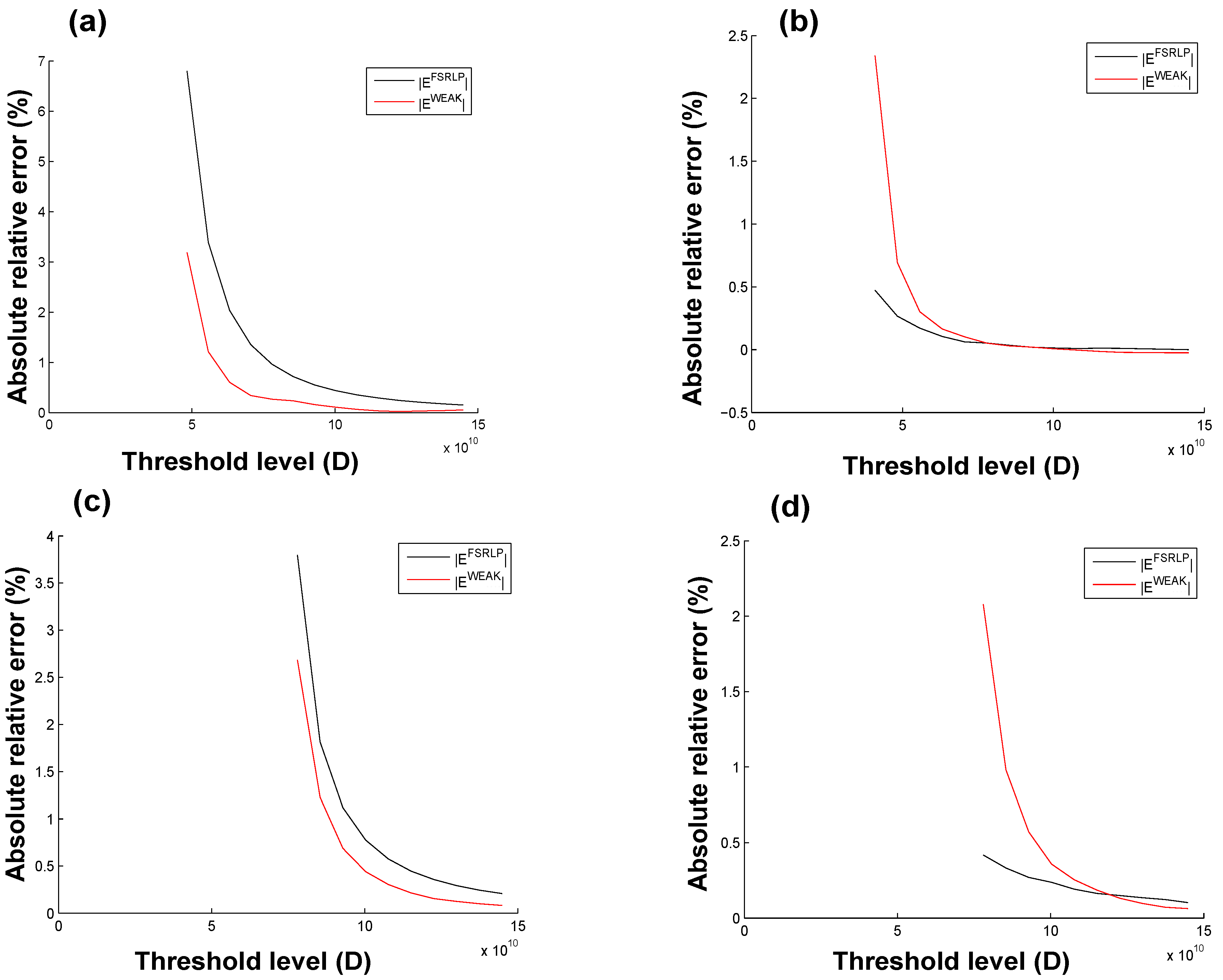
Absolute relative error comparisons for each severity distribution, for: (a) GP distributed losses in the ZCB case (and the CP case in (b)); and (c) Burr distributed losses in the index-linked ZC CAT bond case (and the index-linked CP CAT bond case in (d)), for year. Note the different threshold levels, for each severity distribution, from which the weak approximation became applicable.
Figure A3.
Absolute relative error comparisons for each severity distribution, for: (a) GP distributed losses in the ZCB case (and the CP case in (b)); and (c) Burr distributed losses in the index-linked ZC CAT bond case (and the index-linked CP CAT bond case in (d)), for year. Note the different threshold levels, for each severity distribution, from which the weak approximation became applicable.

References
- Artemis. 2016. Catastrophe Bond and Insurance-Linked Securities Deal Directory. Available online: http://www.artemis.bm/deal_directory/ (accessed on 15 December 2017).
- Baryshnikov, Yuliy, Anita Mayo, and David R. Taylor. 1998. Pricing of CAT Bonds. Working Paper. Available online: http://citeseerx.ist.psu.edu/viewdoc/download?doi=10.1.1.202.9296&rep=rep1&type=pdf (accessed on 15 December 2017).
- Beard, Robert. 2013. Risk Theory: The Stochastic Basis of Insurance. Berlin: Springer, Volume 20. [Google Scholar]
- Billingsley, Patrick. 2013. Convergence of Probability Measures. New York: John Wiley & Sons. [Google Scholar]
- Bodoff, Neil M., and Yumbo Gan. 2009. An Analysis of the Market Price of CAT Bonds. Casualty Actuarial Society E-Forum. Available online: https://www.casact.org/pubs/forum/09spforum/02Bodoff.pdf (accessed on 15 December 2017).
- Braun, Alexander. 2011. Pricing catastrophe swaps: A contingent claims approach. Insurance: Mathematics and Economics 49: 520–36. [Google Scholar] [CrossRef]
- Braun, Alexander. 2016. Pricing in the primary market for CAT bonds: New empirical evidence. The Journal of Risk and Insurance 83: 811–47. [Google Scholar] [CrossRef]
- Burnecki, Krzysztof. 2000. Self-similar processes as weak limits of a risk reserve process. Probability and Mathematical Statistics 20: 261–72. [Google Scholar]
- Burnecki, Krzysztof, and Mario Giuricich. 2017. Pricing catastrophe bonds based on a left-truncated loss index. Available online: https://papers.ssrn.com/sol3/papers.cfm?abstractid=2973419 (accessed on 15 December 2017).
- Burnecki, Krzysztof, and Grzegorz Kukla. 2003. Pricing of zero-coupon and coupon CAT bonds. Applicationes Mathematicae (Warsaw) 30: 315–24. [Google Scholar] [CrossRef]
- Burnecki, Krzysztof, Adam Misiorek, and Rafał Weron. 2005. Loss distributions. In Statistical Tools for Finance and Insurance. Edited by Pavel Čižek, Wolfgang Härdle and Rafał Weron. Berlin: Springer, pp. 289–317. [Google Scholar]
- Calderín-Ojeda, Enrique, Kevin Fergusson, and Xueyuan Wu. 2017. An EM Algorithm for Double-Pareto-Lognormal Generalized Linear Model Applied to Heavy-Tailed Insurance Claims. Risks 5: 60. [Google Scholar] [CrossRef]
- Chang, Carolyn W., and Jack S.K. Chang. 2017. An Integrated Approach to Pricing Catastrophe Reinsurance. Risks 5: 51. [Google Scholar] [CrossRef]
- Chaubey, Yogendra P., Jose Garrido, and Sonia Trudeau. 1998. On the computation of aggregate claims distributions: Some new approximations. Insurance: Mathematics and Economics 23: 215–30. [Google Scholar] [CrossRef]
- Cox, Sam, and Hal Pedersen. 2000. Catastrophe risk bonds. North American Actuarial Journal 4: 56–82. [Google Scholar] [CrossRef]
- Cummins, J. David, and Mary A. Weiss. 2009. Convergence of insurance and financial markets: Hybrid and securitized risk-transfer solutions. Journal of Risk and Insurance 76: 493–545. [Google Scholar] [CrossRef]
- Daley, D.J., Edward Omey, and Rein Vesilo. 2007. The tail behavior of a random sum of subexponential random variables and vectors. Extremes 10: 21–39. [Google Scholar] [CrossRef]
- Dassios, Angelos, and Ji-Wook Jang. 2003. Pricing of catastrophe reinsurance and derivatives using the Cox process with shot noise intensity. Finance and Stochastics 7: 73–95. [Google Scholar] [CrossRef] [Green Version]
- Dieckmann, Stephan. 2010. By force of nature: Explaining the yield spread on catastrophe bonds. Available online: https://papers.ssrn.com/sol3/papers.cfm?abstract_id=1082879 (accessed on 15 December 2017).
- Egami, Masahiko, and Virginia R. Young. 2008. Indifference prices of structured catastrophe (CAT) bonds. Insurance: Mathematics and Economics 42: 771–78. [Google Scholar] [CrossRef]
- Embrechts, Paul. 2000. Actuarial versus financial pricing of insurance. The Journal of Risk Finance 1: 17–26. [Google Scholar] [CrossRef]
- Embrechts, Paul, Claudia Klüppelberg, and Thomas Mikosch. 2013. Modelling Extremal Events: For Insurance and Finance. Berlin: Springer, Volume 33. [Google Scholar]
- Embrechts, Paul, and Steffen Meister. 1997. Pricing insurance derivatives, the case of CAT-futures. Proceedings of the 1995 Bowles Symposium on Securitization of Risk, Georgia State University Atlanta, Society of Actuaries, Monograph M-FI97-1. pp. 15–26. Available online: http://citeseerx.ist.psu.edu/viewdoc/summary?doi=10.1.1.493.2001 (accessed on 15 December 2017).
- Esscher, Fredrik. 1932. On the probability function in the collective theory of risk. Scandinavian Actuarial Journal 1932: 175–95. [Google Scholar]
- Furrer, Hansjörg, Zbigniew Michna, and Aleksander Weron. 1997. Stable Lévy motion approximation in collective risk theory. Insurance: Mathematics and Economics 20: 97–114. [Google Scholar] [CrossRef]
- Galeotti, Marcello, Marc Gürtler, and Christine Winkelvos. 2013. Accuracy of premium calculation models for CAT bonds—An empirical analysis. Journal of Risk and Insurance 80: 401–21. [Google Scholar] [CrossRef]
- Gerber, Hans U., and Elias S.W. Shiu. 1996. Actuarial bridges to dynamic hedging and option pricing. Insurance: Mathematics and Economics 18: 183–218. [Google Scholar] [CrossRef]
- Grandell, Jan. 2012. Aspects of Risk Theory. Berlin: Springer. [Google Scholar]
- Härdle, Wolfgang K., and Brenda L. Cabrera. 2010. Calibrating CAT bonds for Mexican earthquakes. Journal of Risk and Insurance 77: 625–50. [Google Scholar] [CrossRef]
- Jaimungal, Sebastian, and Yuxiang Chong. 2014. Valuing clustering in catastrophe derivatives. Quantitative Finance 14: 259–70. [Google Scholar] [CrossRef]
- Janicki, Aleksander, and Aleksander Weron. 1994. Simulation and Chaotic Behaviour of Stable Processes. New York: Marcel Dekker. [Google Scholar]
- Jarrow, Robert A. 2010. A simple robust model for CAT bond valuation. Finance Research Letters 7: 72–79. [Google Scholar] [CrossRef]
- Kohatsu-Higa, Arturo, and Peter Tankov. 2010. Jump-adapted discretization schemes for Lévy-driven SDEs. Stochastic Processes and their Applications 120: 2258–85. [Google Scholar] [CrossRef]
- Lane, Morton N. 2003. Rationale and Results with the LFC Cat Bond Pricing Model. Chicago: Lane Financial Ltd. [Google Scholar]
- Lane, Morton N., and Olivier Mahul. 2008. Catastrophe Risk Pricing: An Empirical Analysis. Working Paper. Washington: The World Bank, Available online: https://openknowledge.worldbank.org/handle/10986/6900 (accessed on 15 December 2017).
- Lee, Jin-Ping, and Min-Teh Yu. 2002. Pricing default-risky CAT bonds with moral hazard and basis risk. Journal of Risk and Insurance 69: 25–44. [Google Scholar] [CrossRef]
- Lindvall, Torgny. 1973. Weak convergence of probability measures and random functions in the function space d [0,∞). Journal of Applied Probability 10: 109–21. [Google Scholar] [CrossRef]
- Loubergé, Henri, Evis Kellezi, and Manfred Gilli. 1999. Using catastrophe-linked securities to diversify insurance risk: A financial analysis of CAT bonds. Journal of Insurance Issues, 125–46. [Google Scholar]
- Ma, Zong-Gang, and Chao-Qun Ma. 2013. Pricing catastrophe risk bonds: A mixed approximation method. Insurance: Mathematics and Economics 52: 243–54. [Google Scholar] [CrossRef]
- Merton, Robert C. 1976. Option pricing when underlying stock returns are discontinuous. Journal of Financial Economics 3: 125–44. [Google Scholar] [CrossRef]
- Michna, Zbigniew. 2005. On approximations of risk process with renewal arrivals in alpha-stable domain. Probability and Mathematical Statistics 25: 173. [Google Scholar]
- Nolan, John P. 2015. Stable Distributions—Models for Heavy Tailed Data. Boston: Birkhauser, In Progress, Chapter 1. Available online: http://fs2.american.edu/jpnolan/www/stable/stable.html (accessed on 15 December 2017).
- Nowak, Piotr, and Maciej Romaniuk. 2013. Pricing and simulations of catastrophe bonds. Insurance: Mathematics and Economics 52: 18–28. [Google Scholar] [CrossRef]
- Pentikäinen, Teivo. 1977. On the approximation of the total amount of claims. Astin Bulletin 9: 281–89. [Google Scholar]
- Peters, Gareth W., and Pavel V. Shevchenko. 2015. Advances in Heavy Tailed Risk Modeling: A Handbook of Operational Risk. New York: John Wiley & Sons. [Google Scholar]
- Reshetar, Ganna. 2008. Pricing of multiple-event coupon paying CAT bond. Available online: https://papers.ssrn.com/sol3/papers.cfm?abstract_id=1059021 (accessed on 15 December 2017).
- Samorodnitsky, Gennady, and Murad S. Taqqu. 1994. Stable Non-Gaussian Random Processes. London: Chapman & Hall. [Google Scholar]
- Schmidt, Thorsten. 2014. Catastrophe insurance modeled by shot-noise processes. Risks 2: 3–24. [Google Scholar] [CrossRef] [Green Version]
- Seal, Hilary L. 1977. Approximations to risk theory’s F(x,t) by means of the gamma distribution. Astin Bulletin 9: 213–18. [Google Scholar] [CrossRef]
- Seri, Raffaello, and Christine Choirat. 2015. Comparison of approximations for compound Poisson processes. Astin Bulletin 45: 601–37. [Google Scholar] [CrossRef]
- Skorokhod, Anatoliy V. 1957. Limit theorems for stochastic processes with independent increments. Theory of Probability & Its Applications 2: 138–71. [Google Scholar]
- Stam, A.J. 1973. Regular variation of the tail of a subordinated probability distribution. Advances in Applied Probability 5: 308–27. [Google Scholar] [CrossRef]
- Sundt, Bjørn. 1982. Asymptotic behavior of compound distributions and stop-loss premiums. Astin Bulletin 13: 89–98. [Google Scholar] [CrossRef]
- Vaugirard, Victor E. 2003a. Pricing catastrophe bonds by an arbitrage approach. The Quarterly Review of Economics and Finance 43: 119–32. [Google Scholar] [CrossRef]
- Vaugirard, Victor E. 2003b. Valuing catastrophe bonds by Monte Carlo simulations. Applied Mathematical Finance 10: 75–90. [Google Scholar] [CrossRef]
- Vaugirard, Victor E. 2004. A canonical first passage time model to pricing nature-linked bonds. Economics Bulletin 7: 1–7. [Google Scholar]
- Wang, Shaun S. 2000. A class of distortion operators for pricing financial and insurance risks. Journal of risk and insurance 67: 15–36. [Google Scholar] [CrossRef]

Table 1.
Parametric severity distributions considered, defined on the non-negative real numbers.
| Distribution | Parameterization | Constraints |
|---|---|---|
| Burr type XII | ||
| Generalized Pareto | ||
| Modified generalized extreme value | ||
Table 2.
Values of , and d for the selected severity distributions.
| Distribution | d | ||
|---|---|---|---|
| 1 | |||
| 1 | |||
| 1 |
Table 3.
Estimated parameters for three severity distributions (Burnecki and Giuricich 2017).
Table 3.
Estimated parameters for three severity distributions (Burnecki and Giuricich 2017).
| Distribution | Estimated Parameters |
|---|---|
Table 4.
Comparison of index-linked zero-coupon (ZC) catastrophe (CAT) bond prices, under the weak approximation, MC estimation and the first-order single risk loss process (FSRLP) approximation, for different threshold levels D and different underlying loss severity distributions. GP, generalized Pareto.
| D | Severity Distribution | MC Price | ||
|---|---|---|---|---|
| (%) | (%) | |||
| GP | ||||
| GP | ||||
| GP | ≈0 | |||
| Burr | ||||
| Burr | ||||
| Burr | ≈0 | ≈0 |
Table 5.
Comparison of index-linked CP CAT bond prices, under the weak approximation, MC estimation and the FSRLP approximation, for different threshold levels and different underlying loss severity distributions.
Table 5.
Comparison of index-linked CP CAT bond prices, under the weak approximation, MC estimation and the FSRLP approximation, for different threshold levels and different underlying loss severity distributions.
| Severity Distribution | MC Price | |||
|---|---|---|---|---|
| (%) | (%) | |||
| GP | ||||
| GP | ≈0 | ≈0 | ||
| GP | ≈0 | ≈0 | ||
| Burr | ||||
| Burr | ||||
| Burr | ≈0 | ≈0 |
© 2017 by the authors. Licensee MDPI, Basel, Switzerland. This article is an open access article distributed under the terms and conditions of the Creative Commons Attribution (CC BY) license (http://creativecommons.org/licenses/by/4.0/).
Share and Cite
MDPI and ACS Style
Burnecki, K.; Giuricich, M.N. Stable Weak Approximation at Work in Index-Linked Catastrophe Bond Pricing. Risks 2017, 5, 64. https://doi.org/10.3390/risks5040064
AMA Style
Burnecki K, Giuricich MN. Stable Weak Approximation at Work in Index-Linked Catastrophe Bond Pricing. Risks. 2017; 5(4):64. https://doi.org/10.3390/risks5040064
Chicago/Turabian StyleBurnecki, Krzysztof, and Mario Nicoló Giuricich. 2017. "Stable Weak Approximation at Work in Index-Linked Catastrophe Bond Pricing" Risks 5, no. 4: 64. https://doi.org/10.3390/risks5040064
Note that from the first issue of 2016, this journal uses article numbers instead of page numbers. See further details here.