Longevity Risk Management and the Development of a Value-Based Longevity Index

Abstract

The design and development of post-retirement income products require the assessment of longevity risk, as well as a basis for hedging these risks. Most indices for longevity risk are age-period based. We develop and assess a cohort-based value index for life insurers and pension funds to manage longevity risk. There are two innovations in the development of this index. Firstly, the underlying variables of most existing longevity indices are based on mortality experience only. The value index is based on the present value of future cash flow obligations, capturing all the risks in retirement income products. We use the index to manage both longevity risk and interest rate risk. Secondly, we capture historical dependencies between ages and cohorts with a cohort-based stochastic mortality model. We achieve this by introducing age-dependent model parameters. With our mortality model, we obtain realistic cohort correlation structures and improve the fitting performance, particularly for very old ages.

1. Introduction

Longevity risk is the risk that individuals live longer than expected. Since the 1960s, the life expectancy for 65-year-olds in Europe and North America has increased by about one year each decade (Loeys et al. 2007). For defined benefit (DB) pension plans and insurance companies with significant annuity policies, longevity improvement has become a high-profile risk. It is estimated that the value of U.K. pension liabilities increases by 3–4% with each additional year of life expectancy. Several other factors have contributed to the increasing importance of longevity risk, including lower investment returns, IFRSreporting requirements, regulatory changes (e.g., Solvency II capital requirement) and a lower fertility rate.

Traditional participants in the longevity market include DB pension funds, insurers and re-insurers. The pension funds have a negative exposure to longevity risk because the value of their liabilities increases with life expectancy. Life insurance companies have relatively flat exposure to longevity risk, with annuity portfolios offsetting insurance policies (Loeys et al. 2007). Hence, the market has overall negative exposure to longevity improvements. Re-insurers neither have the capacity, nor are willing to accept such a large risk (Wadsworth 2005). Capital markets, with their depth, capacity and experience in risk hedging, have the potential to hedge longevity risk effectively (Blake et al. 2009).

Longevity risk management products have been introduced by the capital markets since 20081, including customized, indemnity-based hedges and index-based hedges (e.g., q-forward, survivor-forward (s-forward), longevity swaps). Two major longevity indices are J.P. Morgan’s LifeMetrics (launched in 2007 and transferred to Life and Longevity Markets Association in 2010) and Deutsche Börse Xpect-Club Vita Index since 2010. LifeMetrics consist of three underlying components: crude central mortality rates, graduated initial mortality rates and period life expectancy (Coughlan et al. 2007). The index data are classified in terms of country, gender and cohort. Deutsche Börse adds one more dimension to its Xpect Cohort index: the pension amount received, which aims to capture the heterogeneity of socio-economic classes within a particular population (DeutscheBorse 2012). The underlying component of the Xpect Cohort index is the number of survivors for a defined cohort group.

Indemnity-based hedges, by construction, are able to eliminate basis risk and achieve a perfect hedge. Basis risk of longevity refers to the differences between the exposed population and the hedging population; for example, differences in geographic location, gender, age or socio-economic class. For indemnity-based hedges, there are no such differences, and the basis risk is zero. On the other hand, basis risk leads to an imperfect hedge with index-based instruments if the hedging population, which is used to calculate an index, significantly differs from the exposed population for which longevity risk needs to be hedged. The main motivation for index providers to classify index data in terms of country, gender, cohort and/or socio-economic class is to reduce the basis risk.

Despite the existence of basis risk, index-based hedging instruments have several advantages over customized hedges. Firstly, with publicly-available national population data, a longevity index offers transparency to investors who seek low correlations of longevity products with other asset classes for a reasonable return. For index hedges, investors need limited expertise in the actuarial information in the books of pension funds or insurance companies. Therefore, information asymmetry (different parties involved in one transaction do not have the same level of information) is not an issue in an index-based hedge. Secondly, with the standardised index data and transparency, index hedges can potentially create more liquidity and reduce the cost of hedging. Lastly, the effect of basis risk may have been overestimated (Coughlan et al. 2011).The work in Cairns et al. (2014) proposes that despite differences in demographic profiles, basis risk can be substantially reduced due to high correlations in mortality improvements (particularly for a long hedge horizon) between the exposed populations and the hedging population. The work in Ngai and Sherris (2011) finds that the longevity risk can be substantially reduced for immediate life annuities using static hedging with longevity bonds and q-forwards in the Australian market. Against this background, we develop a value-based longevity index that incorporates both longevity and interest rate risks using a cohort mortality model calibrated to Australian data. We show how the index can be used in hedging a life annuity and how both interest rate and longevity risk can be effectively hedged.

2. Value-Based Longevity Index

The underlying variable in most current longevity indices (i.e., LifeMetrics and Xpect-Club Vita Index) is based on the mortality experience of a given population. From the annuity pricing perspective, it is more suitable for the underlying index to reflect the value of future obligations (Sherris and Wills 2008). We develop a cohort-based value index suitable for hedging the present value of a series of future cash flows dependent on future mortality and interest rates. The importance of value hedging is particularly important with the capital charge introduced by Solvency II, which uses the change in net asset value. Value hedging is appropriate for a range of annuity products including hedging deferred annuities.

Interest rate risk is inherent in a value-based strategy; however, in studies focussing on the hedging effectiveness of index-based strategies, it is not considered in conjunction with mortality risk. For example, Coughlan et al. (2011) and Cairns et al. (2014) assume constant interest rates, and Blackburn and Sherris (2014) assume fixed forward interest rates. In practice, such assumptions are unrealistic, and the interaction of mortality risk with interest rate risk should be incorporated into hedging analysis. In the value-based strategy, we model both stochastic mortality rates and interest rates. We propose that the advantage of a value-based index with the present value (PV) of future cash flows as the underlying relation, over a mortality-based index, is that the value index allows one to consider both mortality risk and interest rate risk in the hedging in a consistent manner.

We are motivated by Sherris (2009), who constructs a value-based index that takes into account both mortality and economic factors that is relevant to individuals who are self-insuring their mortality risk. The work in Sherris (2009) proposes a longevity index that reflects the PV of providing a unit indexed income stream to individuals to the age when they will be 95% confident of covering their longevity risk. In contrast, the index we construct is relevant to life insurers and pension funds and is based on a life annuity with a nominal annual payment similar to the products commonly offered by life insurers. We consider the full age range, up to age 120, and consider only nominal cash flows.

The value index is cohort based and considers cohorts with varying starting ages. For this, we develop a cohort-based model with stochastic mortality intensity. A number of studies has proposed continuous-time, affine stochastic mortality models for a single cohort, e.g., (Dahl 2004; Biffis 2005; Schrager 2006; Luciano and Vigna 2008). In the age-period affine mortality model of Blackburn and Sherris (2013), perfect correlations across multiple cohorts are implicitly assumed. The work in Jevtic et al. (2013) notes that empirically, cohort correlations are imperfect and attempts to capture this property with their cohort-based affine mortality model. They use a two-factor Ornstein–Uhlenbeck process to calibrate the mortality surface, with a common factor for all cohorts and a cohort-specific factor.

Motivated by Jevtic et al. (2013), we develop a cohort model with more realistic correlations. The calibration results in Jevtic et al. (2013) appear unrealistically high; the correlation matrix is constant and independent of the initial age; and the calibrated parameters result in large out-of-sample forecasting errors for old ages (age 80 and beyond). The high correlations appear to result from the common factor, which introduces high dependence across cohorts. Since the drift and diffusion coefficients are age-independent, the model is unable to produce a richer, initial age-dependent correlation structure. We address these issues and develop an improved cohort-based model motivated by Jevtic et al. (2013).

We use the affine term structure model (ATSM) (Duffie and Kan 1996) for both mortality and interest rates. Special cases of the ATSM, such as the Vasicek model (Vasicek 1977) and the Cox–Ingersoll–Ross (CIR) model (Cox et al. 1985), provide analytical solutions of zero-coupon bond and longevity bond prices. These models focus on the time series property of the term structures rather than the initial cross-sectional property (Bolder 2001). The ATSM provides analytical tractability, ease of implementation and a focus on future evolutions of mortality rates and interest rates. We make the assumption that mortality risk and interest rate risk are independent. We calibrate the proposed models to mortality and interest rate data. Based on estimated model parameters, we construct the value index and evaluate the effectiveness of index-based hedging strategies.

The remainder of this paper is organized as follows. Section 3 presents an analysis of the mortality data. Section 4 presents the mortality model and gives details of its calibration. Section 5 presents the interest rate model and its calibration. Section 6 gives the detail of the the value-based index and presents an analysis of its hedge effectiveness. Finally, Section 7 concludes.

3. Mortality Data Analysis

An important aspect of our value-based longevity index is the model for mortality. In particular, we focus on providing a more realistic model for the age-dependent trend, volatility and correlation. We present here the analyses of the historical mortality data in order to propose a stochastic, cohort-based mortality model that is consistent with our empirical findings. In particular, we aim to identify the potential dependence of mortality parameters on the initial age and how cohorts are correlated empirically. To this end, we choose Australian male data from the Human Mortality Database (HMD) and collect for each cohort the mortality rates from ages 49–99. The 1890, 1895, 1900 and 1905 cohorts are selected.

For each cohort, we approximate the continuous-time mortality intensity $\mu (t,x)$ for an individual aged x at t with the crude death rate $m_c(t,x)=\frac{D(t,x)}{E(t,x)}$, where $D(t,x)$ and $E(t,x)$ respectively represent the number of deaths and average population exposure during calendar year t aged x last birthday. We then calculate mortality intensities for each cohort and model the change in mortality rates as each cohort ages. The mortality intensity change is defined as $▵\mu (t,x)=\mu (t+1,x+1)-\mu (t,x)$. Hence, for each cohort, we have 50 observations of $▵\mu (t,x)$. We choose $▵\mu (t,x)$ for our analyses in order to de-trend the mortality rates of the different cohorts. The work in Njenga and Sherris (2011) shows that, for statistical reasons, differences in mortality rates or mortality trends should be modelled, and due to the trending of cohorts, the number of factors required to explain a given level of total variance is higher for the differences of the mortality levels than for the levels themselves.

3.1. Drift of Mortality Intensity

We first consider the behaviour of the drift parameter of the mortality intensity. To investigate potential age dependence, we separate total observations into three age groups: 50–64, 65–84, 85–99. We do so in order to capture the effects of mid-initial age 50, old initial age 65 and very old initial age 85. We then calculate the average of $▵\mu (t,x)$ within each group. In doing so, we approximate the continuous-time drift with its discrete-time counterpart. The results are presented in

Table 1. Drift of mortality intensity by cohort.

Initial Age	1890	1895	1900	1905
50	0.001425	0.001639	0.001977	0.001800
65	0.007501	0.005820	0.005335	0.005601
85	0.016177	0.017104	0.015258	0.017705

.

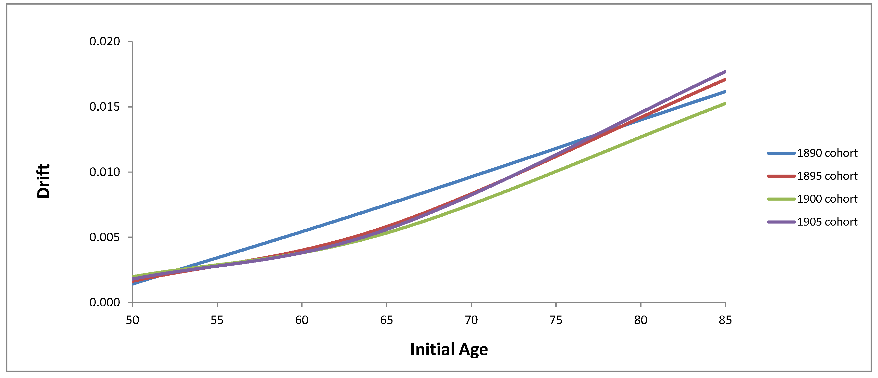
From Table 1, we clearly observe within each cohort the initial age dependence of the drift. In Figure 1, we plot the drift as a function of the initial age. By observation, we see that a linear function of age fits the observed drifts well. We hence propose to use the functional form $a+bx$ to represent the initial age dependent drift, where a and b are constants and x is the age.

3.2. Volatility of Mortality Intensity

For each cohort, we calculate the standard deviation of $▵\mu (t,x)$ within each age group to approximate the continuous-time volatility of mortality intensity. Results summarized in

Table 2. Volatility of mortality intensity by cohort.

Initial Age	1890	1895	1900	1905
50	0.001031	0.000965	0.001748	0.001343
65	0.007080	0.005082	0.007610	0.005494
85	0.030253	0.031574	0.033655	0.024272

show the dependence of volatility on the initial age. Figure 2 shows that the volatility approximately increases exponentially with age. We propose to use the functional form $e^{(c+dx)}$ to represent the age-dependent volatility, where c and d are constants.

3.3. Cohort Correlations

We consider the 20-year correlation of $▵\mu (t,x)$ across cohorts starting from the same calendar time and following the differing cohorts through time. In order to examine whether correlations are constant with initial age, we calculate the correlation matrix at four different calendar times: 1955, 1960, 1965 and 1970. Our correlation matrix therefore is based on a fixed calendar time and a fixed time horizon with mortality rates for the differing cohorts observed through time. This differs from the instantaneous cohort correlation structure of Jevtic et al. (2013), which fixes the initial age at 40 for all cohorts.

The correlation matrices are presented in

Table 3. Twenty-year cohort correlations.

Calendar Time 1955
Cohort	1890	1895	1900	1905
1890	1.0000
1895	0.6124	1.0000
1900	0.5157	0.4758	1.0000
1905	0.4271	0.1857	0.5568	1.0000
Calendar Time 1960
1890	1.0000
1895	0.4707	1.0000
1900	0.1489	0.2728	1.0000
1905	0.2103	0.1968	0.0949	1.0000
Calendar Time 1965
1890	1.0000
1895	0.6583	1.0000
1900	0.2881	0.4585	1.0000
1905	0.4376	0.4899	0.5200	1.0000
Calendar Time 1970
1890	1.0000
1895	0.4468	1.0000
1900	0.3600	0.4117	1.0000
1905	0.2401	0.7432	0.6260	1.0000

. We obtain two important findings. Firstly, the historical correlation matrix changes as we change the calendar time, which suggests that correlations change when initial ages change. Secondly, the correlations are lower than those calibrated in Jevtic et al. (2013). Correlations can be calculated by fixing either the calendar time or by fixing the initial age. Both approaches result in empirical correlations significantly lower than the those calibrated by Jevtic et al. (2013), which we find with Australian data. We see that empirically, the cohort correlations exhibit dependence on the initial age. They are also significantly lower than almost perfect correlations. In this study, we aim to capture these empirical features with our mortality model using the age-dependent trend and volatility.

3.4. Principal Component Analysis

The last analysis we carry out is principal component analysis (PCA) on $▵\mu (t,x)$. Results show that three principal components (PCs) are required to explain more than 99% of the total variance of the four cohorts. This contrasts with two PCs for 11 cohorts in Jevtic et al. (2013). It should be noted that, in their study, PCA is applied to the average force of mortality, not the change of mortality. We perform PCA to the mortality rate change of the same U.K. male data, and nine PCs are needed to explain 99% of the total variances of 11 cohorts. These differences are consistent with the finding in Njenga and Sherris (2011), who show that more factors are required to explain the total variance of the differenced mortality rates as compared to the level of mortality rates.

4. Mortality Model

The mortality model we propose is an age-dependent, cohort-based mortality model that aims to reflect the empirical analysis presented in Section 3. The model is non-mean reverting with correlated Gaussian factors. The work in Luciano and Vigna (2005) shows that non-mean reverting processes are more suitable than mean-reverting processes for modelling mortality intensities. The Gaussian factor model is chosen for its analytical tractability and ease of implementation. In order to maintain model tractability, we restrict the number of factors to two2. Though negative mortality intensity is theoretically possible for Gaussian models, in practice, the probability is low (see Blackburn and Sherris (2014) and Brigo and Mercurio (2006) for the interest rate case).

4.1. Model Development

Consider a probability space ($\mathsf{\Omega }$, $\mathcal{F}$, ${\mathcal{F}}_t(t\ge 0)$, P) that satisfies the usual hypothesis that the filtration ${\mathcal{F}}_t(0\le t\le T)$ is right continuous with left limits and P is the real-world probability measure. We calibrate our model to historical data, and so, we use the P measure for this. When we apply the model to value the index, we will require a Q or risk-adjusted pricing measure.

The mortality rate, ${\mu }^i(t,x)$, is a predictable process on this probability space and represents the mortality intensity for individuals aged x at calendar time t of cohort i. Within cohort i, an individual’s death time is the first jump time of a Cox process with intensity ${\mu }^i(t,x)$. Two factors of ${\mu }^i(t,x)={\mu }_1^i(t,x)+{\mu }_2^i(t,x)$ respectively follow the SDEs:

$$d{\mu }_1^i(t,x)={\psi }_1^i(t,x){\mu }_1^i(t,x)dt+{\sigma }_1^i(t,x)d{W}_1^i(t),$$

(1)

$$d{\mu }_2^i(t,x)={\psi }_2^i{\mu }_2^i(t,x)dt+{\sigma }_2^{i}d{W}_2^i(t),$$

(2)

where:

$${\psi }_1^i(t,x)=a+bx,$$

(3)

and:

$${\sigma }_1^i(t,x)=e^{(c+dx)}.$$

(4)

$W_1^i$ and $W_2^i$ are correlated Brownian motions on P and $d{W}_1^{i}d{W}_2^i={\rho }^{i}dt$. The instantaneous correlation between any two ages, reflecting the mortality of two different cohorts at the same time, is readily derived from this. However, we consider correlations between cohorts across time and calibrate our parameters to fit these historical correlations.

Using the Cholesky decomposition of the correlation matrix of $W_1^i$ and $W_2^i$, we transform Equations (3) and (4) into factors driven by:

$$d{\mu }_1^i(t,x)={\psi }_1^i(t,x){\mu }_1^i(t,x)dt+{\sigma }_1^i(t,x)d{Z}_1(t),$$

(5)

$$d{\mu }_2^i(t,x)={\psi }_2^i{\mu }_2^i(t,x)dt+{\sigma }_2^i{\rho }^{i}d{Z}_1(t)+{\sigma }_2^i\sqrt{1-{({\rho }^i)}^2}d{Z}_2(t),$$

(6)

In Equations (7) and (8), $Z_1$ and $Z_2$ are two independent Brownian motions. It is clear that once the cohort index i and initial age x are specified, calendar time t is determined by $t=i+x$. As a result, the functional forms of ${\psi }_1^i(t,x)$ in Equation (5) and ${\sigma }_1^i(t,x)$ in Equation (6) implicitly capture the dependence on t. To keep the the model tractable, ${\psi }_2^i$, ${\sigma }_2^i$ and ${\rho }^i$ are assumed constant for each cohort and independent of the initial age.

For the current setup, the instantaneous mortality intensity of each cohort is3:

$$\begin{array}{cc}\hfill d\mu (t,x)=& d{\mu }_1(t,x)+d{\mu }_2(t,x)\hfill \\ \hfill =& ({\psi }_1(t,x){\mu }_1+{\psi }_2{\mu }_2)dt+({\sigma }_1(t,x)+{\sigma }_2\rho )d{Z}_1(t)\hfill \\ & +{\sigma }_2\sqrt{1-{\rho }^2}d{Z}_2(t).\hfill \end{array}$$

(7)

We make the assumption that ${\psi }_1$ and ${\sigma }_1$ are piecewise constant with respect to each age group and depend on the initial age of the group only. For instance, for the 50–64 age group, ${\psi }_1=a+50b$ and ${\sigma }_1=e^{(c+50d)}$. Hence, within each age group of each cohort, for each $s>t$, if we let $\tau =s-t$ and integrate Equation (9), we get:

$$\begin{array}{cc}\hfill \mu (s,x+\tau )=& {\mu }_1(t,x)e^{{\psi }_1(t,x)\tau }+{\mu }_2(t,x)e^{{\psi }_2\tau }+{\sigma }_1(t,x){\int }_t^s{e}^{{\psi }_1(t,x)(s-u)}d{Z}_1(u)\hfill \\ & +{\sigma }_2\rho {\int }_t^s{e}^{{\psi }_2(s-u)}d{Z}_1(u)+{\sigma }_2\sqrt{1-{\rho }^2}{\int }_t^s{e}^{{\psi }_2(s-u)}d{Z}_2(u).\hfill \end{array}$$

(8)

The survival probability from t to s, provided the individual is alive at t and aged x, is given by4:

$$\begin{array}{cc}\hfill P(t,s)=& E(e^{-{\int }_t^s\mu (u)d(u)}|{\mathcal{F}}_t)\hfill \\ \hfill =& \exp \left[\frac{1-e^{{\psi }_1(t,x)\tau }}{{\psi }_1(t,x)}·{\mu }_1(t,x)+\frac{1-e^{{\psi }_2\tau }}{{\psi }_2}·{\mu }_2(t,x)+\frac{1}{2}V(\tau )\right].\hfill \end{array}$$

(9)

where,

$$\begin{array}{cc}\hfill V(\tau )=& \frac{{\sigma }_1^2}{{\psi }_1^2}\left[\tau -\frac{2}{{\psi }_1}{e}^{{\psi }_1\tau }+\frac{e^{2{\psi }_1\tau }}{2{\psi }_1}+\frac{3}{2{\psi }_1}\right]\hfill \\ \hfill +& \frac{{\sigma }_2^2}{{\psi }_2^2}\left[\tau -\frac{2}{{\psi }_2}{e}^{{\psi }_2\tau }+\frac{e^{2{\psi }_2\tau }}{2{\psi }_2}+\frac{3}{2{\psi }_2}\right]\hfill \\ \hfill +& 2\rho \frac{{\sigma }_1{\sigma }_2}{{\psi }_1{\psi }_2}\left[\tau -\frac{e^{{\psi }_1\tau }-1}{{\psi }_1}-\frac{e^{{\psi }_2\tau }-1}{{\psi }_2}+\frac{e^{({\psi }_1+{\psi }_2)\tau }-1}{{\psi }_1+{\psi }_2}\right].\hfill \end{array}$$

(10)

We have developed a model that captures the age-varying mortality rate trend and volatility and has a correlation structure that can also capture the age-dependence observed in the historical data. The model is tractable and provides closed-from expressions for survival probabilities.

4.2. Calibration

We calibrate the model parameters by fitting the survival probabilities given by Equation (11) to the observed survival probabilities for the data in Section 3, where we divided our data into four cohorts and three age groups. Within each age group, the actual survival probability $\tilde{P}(t,s)$ is calculated by:

$$\tilde{P}(t,s)=\prod _{i=1}^{\tau }{e}^{-\tilde{\mu }(t+i-1,x+i-1)},$$

(11)

where $\tilde{\mu }(·,·)$ are actual mortality intensities approximated by the crude death rates $m_c(t,x)$. We then minimize the sum of mean square error between $P(t,s)$ and $\tilde{P}(t,s)$ across all four cohorts and three age groups. $\tau =15$ for the 50–64 group and 85–99 group, and $\tau =20$ for the 65–84 group. We therefore minimize the objective function:

$$G=\sqrt{\sum _{j=1}^{200}{W}_j{(P_j(t,s)-{\tilde{P}}_j(t,s))}^2},$$

(12)

where $W_j$ is the weight assigned to the j-th squared error term. We fit to 200 actual survival probabilities in total. We choose non-equal weights by assigning the highest weights to the 50–64 group, medium weights to the 65–84 group and the lowest weights to the 85–99 group. We use lower weights as the initial age increases because the volatility of mortality rates increases significantly with age, which can be seen from the data analyses in Section 2. Hence, an equal-weight calibration scheme tends to over-fit the “noise”. To determine the weights, we sum the inverse of the initial ages as:

$$\mathrm{Sum}=\frac{1}{50}\times 15\times 4+\frac{1}{65}\times 20\times 4+\frac{1}{85}\times 15\times 4.$$

(13)

We then calculate each weight $W_j$ as a proportion of the sum. For each age group across all cohorts, the weight is constant at $\frac{1}{\mathrm{initial}\mathrm{age}\times \mathrm{Sum}}$. Hence, ${\sum }_{j=1}^{200}{W}_j=1$.

In this model, the cohort-specific parameters include ${\psi }_2^i$, ${\sigma }_2^i$, ${\rho }^i$ and initial values of the state variables ${\mu }_1^i(t,x)$ and ${\mu }_2^i(t,x)$. The parameters common to all cohorts are a, b, c and d. Since we consider three different initial ages, in total, there are 40 parameters to estimate. The fit of the model proves to be generally good even with the estimation of this number of parameters using our data. This is an issue for many mortality models in practice.

We calibrate the model parameters with nonlinear constrained optimization. One advantage of using optimization for model calibration is that it is relatively computationally inexpensive. The drawback of this approach is that the estimators are sensitive to the initial conditions used in the optimization (see Cairns and Pritchard 2001). Therefore, as the first step, we estimate the initial conditions of the model parameters with the observed drifts and volatilities in Section 2. The initial conditions of ${\psi }_1$ and ${\sigma }_1$ are $a=-0.0205$, $b=0.0004$, $c=-10.32$ and $d=0.0801$. The remaining initial conditions are presented in

Table 4. Initial conditions for optimisation.

Cohort	${\mathit{\psi }}_2$	${\mathit{\sigma }}_2$	$\mathit{\rho }$	${\mathit{\mu }}_1(50)$	${\mathit{\mu }}_1(65)$	${\mathit{\mu }}_1(85)$	${\mathit{\mu }}_2(50)$	${\mathit{\mu }}_2(65)$	${\mathit{\mu }}_2(85)$
1890	0.0032	0.0002	0.7660	0.0091	0.0305	0.1805	0.0091	0.0305	0.1805
1895	0.0011	−0.0001	0.9999	0.0080	0.0326	0.1490	0.0080	0.0326	0.1490
1900	0.0151	0.0017	0.9999	0.0079	0.0375	0.1442	0.0079	0.0375	0.1442
1905	0.0031	−0.0041	0.8377	0.0074	0.0344	0.1465	0.0074	0.0344	0.1465

. We also impose the constraint in the optimisation that $-1\le {\rho }^i\le 1$.

4.3. Calibration Results

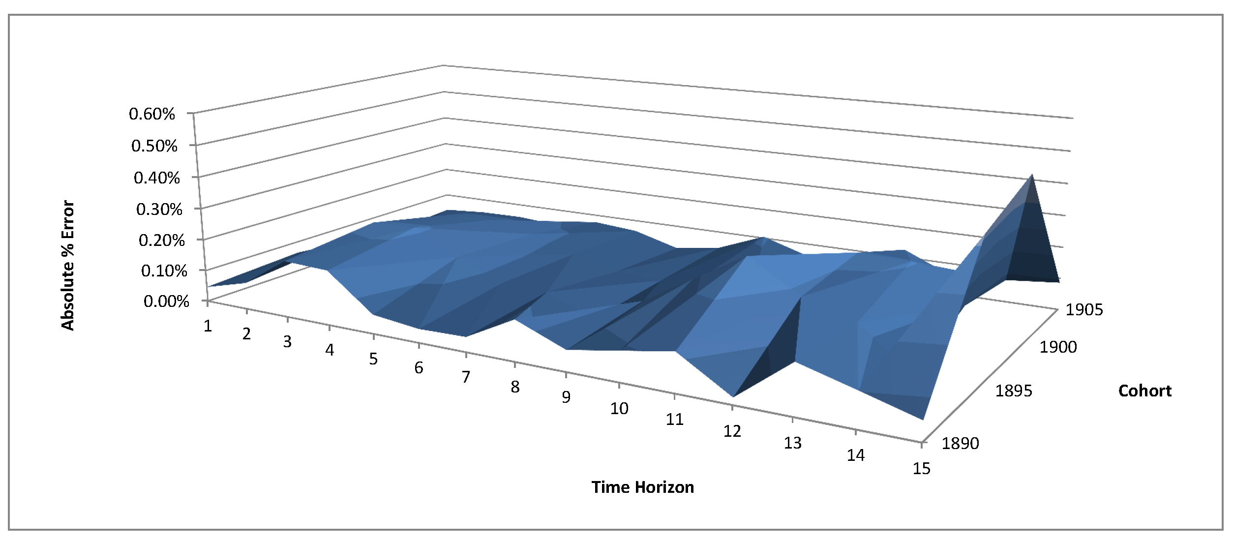
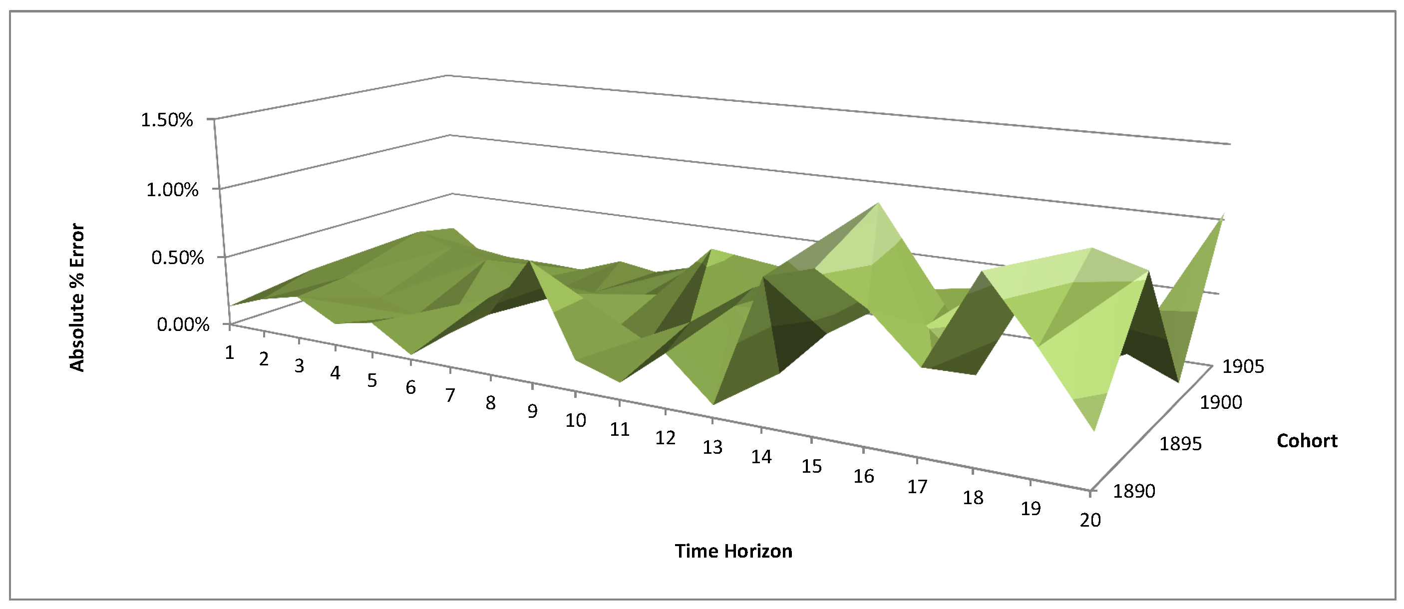
The optimisation results are summarized in

Table 5. Initial age-dependent parameters.

a	b	c	d
0.2280	−0.0037	−10.3270	0.0343

(age-dependent parameters) and

Table 6. Cohort parameters.

Cohort	${\mathit{\psi }}_2$	${\mathit{\sigma }}_2$	$\mathit{\rho }$	${\mathit{\mu }}_1(50)$	${\mathit{\mu }}_1(65)$	${\mathit{\mu }}_1(85)$	${\mathit{\mu }}_2(50)$	${\mathit{\mu }}_2(65)$	${\mathit{\mu }}_2(85)$
1890	0.0721	−0.0001	0.7306	−0.0068	−0.0145	0.0227	0.0157	0.0460	0.1528
1895	0.0632	−0.0073	0.8710	−0.0368	−0.0292	−0.0343	0.0444	0.0607	0.1844
1900	0.0598	0.0000	0.9767	−0.0241	−0.0045	−0.0255	0.0321	0.0449	0.1815
1905	0.0817	−0.0000	0.8482	−0.0072	0.0106	−0.0011	0.0146	0.0256	0.1409

(cohort specific parameters). The fitting performance of the calibrated parameters to the observed survival probabilities is measured by the absolute level of the percentage error $\left|\frac{\tilde{P}(t,s)-P(t,s)}{\tilde{P}(t,s)}\right|$. In Figure 3, Figure 4 and Figure 5, we plot the fitting errors for each age group.

We see that for the age groups 50–64 and 65–84, the fitting errors in general are below 1%. For the very old age group 85–99, the largest fitting error is 11.30%, and only five out of 60 errors are above 5%. Such error levels are in line with the three-factor age-period model results in Blackburn and Sherris (2013), who introduce a third factor to capture the variation in the survival curve for ages over 85. The out-of-sample forecasting in Jevtic et al. (2013) reports 26% fitting error at age 80 and sharp increases afterwards. We attribute the relative fitting performance of our two-factor Gaussian model to the age-dependent parameters. As reflected in the empirical data analyses, the drift and volatility of the mortality rate increase with age. Therefore, the model in Jevtic et al. (2013) with constant parameters is unable to capture the parameter variations as initial age changes.

Based on the parameters in Table 5 and Table 6, we generate mortality rates with Equation (10) with Monte Carlo simulations. No negative mortality rates are produced from the simulations, even though in the optimisation scheme, no positivity constraints of the mortality rates are imposed. This is consistent with the observation in Jevtic et al. (2013) that theoretically, Gaussian models may lead to negative rates; the probability is nevertheless low.

We also investigate whether the simulated mortality rates produce a more realistic correlation structure compared to the historical data using the correlations for varying fixed initial ages over 20-year horizons. To this end, we recalculate the model correlations with the simulated mortality rates and present them in

Table 7. Cohort correlations with simulated mortality rates.

Calendar Time 1955
Cohort	1890	1895	1900	1905
1890	1.0000
1895	0.4710	1.0000
1900	0.3427	0.4019	1.0000
1905	0.5471	0.6195	0.5193	1.0000
Calendar Time 1960
1890	1.0000
1895	−0.1862	1.0000
1900	0.3584	−0.1156	1.0000
1905	0.6125	−0.2554	0.5283	1.0000
Calendar Time 1965
1890	1.0000
1895	0.2348	1.0000
1900	0.6964	0.2709	1.0000
1905	0.8403	0.2587	0.7707	1.0000
Calendar Time 1970
1890	1.0000
1895	0.4367	1.0000
1900	0.7740	0.4174	1.0000
1905	0.9324	0.4593	0.8174	1.0000

.

In Table 7, the 20-year correlations across cohorts show significant variations when we vary calendar time, with varying initial ages of cohorts. Furthermore, these correlations are much lower than those calibrated by Jevtic et al. (2013), which are close to positive perfect correlations (i.e., 100%). These two findings are consistent with the historical correlations presented in Table 3, which shows that our model generates a more realistic correlation structure for mortality rates across time and across cohorts. To examine whether the model correlations in Table 7 fit the realized correlations in Table 3, we carry out the t-test and calculate the 95% confidence interval for the correlation coefficients in Table 3. The standard error is ${\sigma }_r=\sqrt{\frac{1-r^2}{n-2}}$, where r is the estimated correlation and $n=20$ is the sample size. The test statistic $t=\frac{r}{{\sigma }_r}$ follows a t-distribution with $n-2$ degrees of freedom. We measure the sum of the fitting errors by the loss function:

$$L=\sum _{i=1}^K{\left[\max ({\rho }^m-{\rho }^u,0)+\max ({\rho }^l-{\rho }^m,0)\right]}^2,$$

(14)

where $K=24$ is the total number of correlations, ${\rho }^m$ is the model correlation and (${\rho }^l,{\rho }^u$) is the 95% confidence interval of the realized correlation. Because the realized correlations are subject to estimation errors, Equation (16) states that if ${\rho }^m$ falls within the 95% confidence interval, the error is set to zero. Therefore, we only have positive error terms if ${\rho }^m$ is below the lower bound or above the upper bound of the interval, when we are 95% confident that the model correlation is different from the estimated realized correlation. The fitting errors are shown in

Table 8. Fitting errors of the model correlations.

Calendar Time 1955
Cohort	1890	1895	B
1895	0
1900	0	0
1905	0	0	0
Calendar Time 1960
1895	0.0484
1900	0	0
1905	0	0	0
Calendar Time 1965
1895	0.0026
1900	0	0
1905	0	0	0
Calendar Time 1970
1895	0
1900	0	0.0391
1905	0	0	0

.

The total sum of fitting errors is 0.09, and we are able to fit 21 model correlations. To measure the relative performance of our model correlations, we use 95% constant correlation5 to fit the realized correlations. Results show that our model reduces the fitting errors by 85.05%. We have shown that a model with age-dependent parameters will produce correlations closer to realized correlations in historical data when measured across cohorts and across time.

5. Interest Rate Model

5.1. Vasicek Model

We choose the Vasicek one-factor process with constant parameters to model stochastic interest rates. The Vasicek model is chosen for its analytical tractability and the mean reversion property. Under the risk-neutral measure, the instantaneous spot rate $r(t)$ follows the stochastic differential equation:

$$dr(t)=k[\theta -r(t)]dt+\sigma d{W}^r(t),r(0)=r_0,$$

(15)

where k is the mean reversion speed, $\theta$ is the long-term average rate, $\sigma$ is the diffusion coefficient and $r(0)$ is the short rate at initiation. All parameters are positive constants. The stochastic integral equation for $r(t)$ is:

$$r(t)=r(s)e^{-k(t-s)}+\theta \left(1-e^{-k(t-s)}\right)+\sigma {\int }_s^t{e}^{-k(t-u)}d{W}^r(u),s\le t.$$

(16)

Conditional upon information up to s, $r(t)$ follows the normal distribution with mean:

$$E(r(t)|{\mathcal{F}}_s)=r(s)e^{-k(t-s)}+\theta \left(1-e^{-k(t-s)}\right),$$

(17)

and variance:

$$Var(r(t)|{\mathcal{F}}_s)={\sigma }^2{\int }_s^t{e}^{-2k(t-u)}du=\frac{{\sigma }^2}{2k}\left(1-e^{-2k(t-s)}\right).$$

(18)

The analytical tractability of the model hence arises from the normal distribution of the short rate $r(t)$. Though the drawback of the normal distribution is that $r(t)$ can become negative with positive probability, in practice, such probabilities are low.

Another advantage of the model is that it naturally fits into the ATSM framework, with the zero-coupon bond price given by:

$$P(t,T)=A(t,T)·e^{-B(t,T)r(t)}.$$

(19)

$A(t,T)$ and $B(t,T)$ are respectively given by:

$$A(t,T)=\exp \left(\left(\theta -\frac{{\sigma }^2}{2k^2}\right)(B(t,T)-T+t)-\frac{{\sigma }^2}{4k}B{(t,T)}^2\right),$$

(20)

and:

$$B(t,T)=\frac{1}{k}\left(1-e^{-k(T-t)}\right).$$

(21)

Hence, the zero-coupon prices can be calculated with analytical functions of the model parameters.

5.2. Data and Calibration

We calibrate the interest rate model parameters with the Australian zero-coupon discount factors sourced from the Reserve Bank of Australia (RBA). The discount factors are published by RBA daily with maturities ranging from three months up to 10 years. The maturity of each discount factor increases by three months from the previous one. Hence, we have a discrete set of 40 maturities. In order to capture the underlying relation of the model parameters and model outputs, we employ a panel dataset from 2 August 2004–31 July 2014. We have 2527 days in the sample and 40 discount factors each day. Overall, there are 101,080 discount factors to fit with the model. Given three constant parameters, it is unrealistic to expect perfect fits to a large number of discount factors. However, our objective is to use a parsimonious and analytically-tractable model to capture the underlying dynamic of interest rates over a relatively long period.

The model is calibrated by non-linear constrained optimisation, which minimizes the mean square error between the model discount factor $P_{(r)}(0,t)$ and the actual discount factor ${\tilde{P}}_{(r)}(0,t)$. The objective function is:

$$G_r=\sqrt{\frac{1}{N}\sum _{i=1}^{2527}\sum _{j=1}^{40}{(P_{(r),i,j}(0,t)-{\tilde{P}}_{(r),i,j}(0,t))}^2},$$

(22)

where $N=$ 101,080 is the total number of discount factors. The initial values of the model parameters we use in the optimisation are estimated with the dataset. Firstly, the mean reversion parameter k is estimated with the half-life of interest rates, which is the time it takes for the interest rate to move half the distance from $r(0)$ towards its long-term average $\theta$ (Guimaraes 2005). Suppose $T(\frac{1}{2})$ is the half-life, and we rearrange the deterministic part of Equation (17) and obtain:

$$\frac{dr(t)}{\theta -r(t)}=kdt.$$

(23)

Integrating both sides of Equation (25), we get:

$${\int }_{r(0)}^{r(T(\frac{1}{2}))}\frac{dr(t)}{\theta -r(t)}={\int }_0^{T(\frac{1}{2})}kdt,$$

(24)

where $r(T(\frac{1}{2}))-\theta =\frac{1}{2}(r(0)-\theta )$. Straightforward calculations then result in:

$$k=\frac{ln(2)}{T(\frac{1}{2})}.$$

(25)

We then estimate k with Equation (27) and sample data. We approximate the short rate $r(t)$ with the three-month forward rate at t implied by the observed discount factors. We then calculate the average $r(t)$ for each maturity over the sample period. The sample average $r(T(\frac{1}{2}))$ is 5.05%, which corresponds to $T(\frac{1}{2})=5$. Hence, our estimated k is $\frac{ln(2)}{5}=0.1386$, which we use as the initial condition for the optimisation. The constraints we impose for the value of k in the optimisation are obtained by letting $T(\frac{1}{2})$ be respectively 0.25 and 10. We also estimate with the sample data the initial conditions and constraints for $\theta$ and $\sigma$. The results are presented in

Table 9. Inputs for the interest rate model calibration.

Inputs	k	$\mathit{\theta }$	$\mathit{\sigma }$
Initial Value	0.1386	0.0542	0.0009
Upper Bound	2.7726	0.0660	0.0043
Lower Bound	0.0693	0.0375	0.0002

.

5.3. Calibration Results

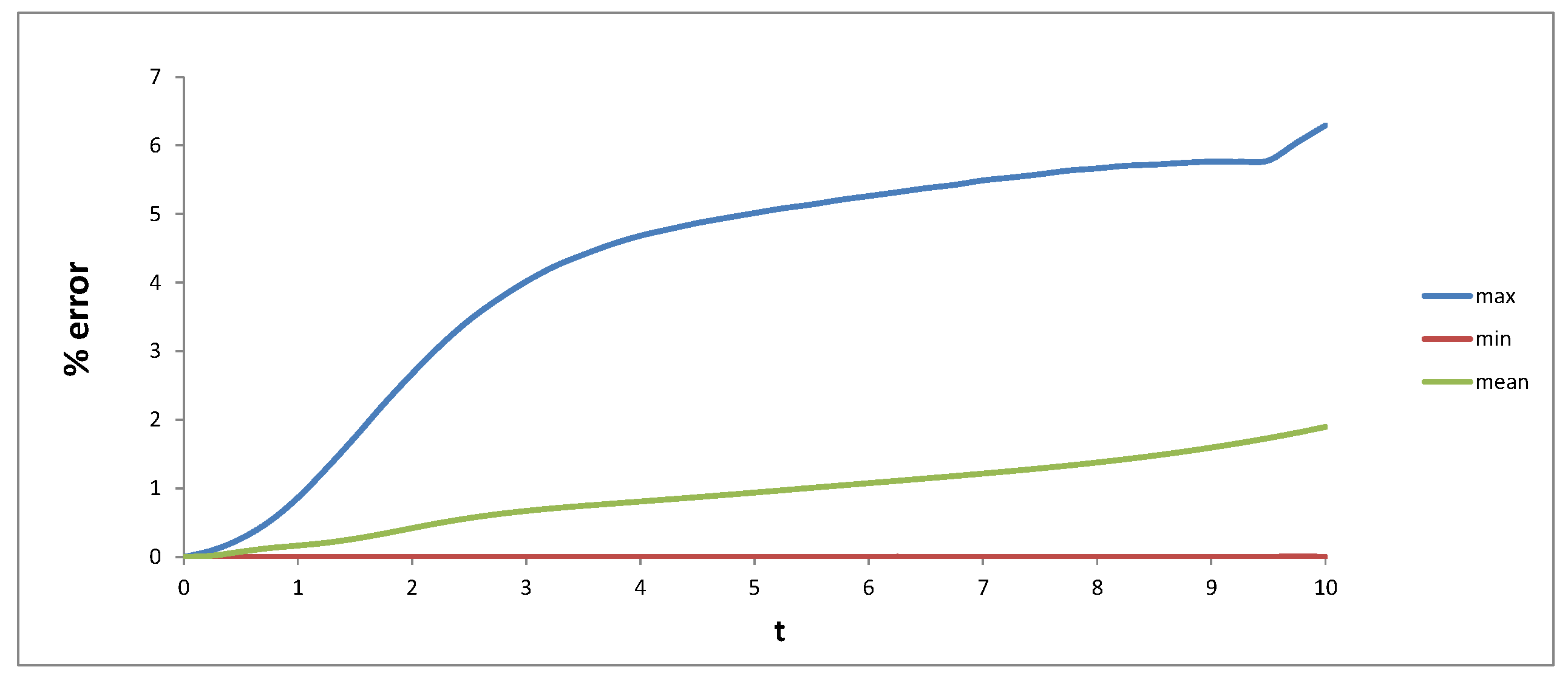
The calibrated parameters with the proposed optimisation scheme are $k=0.1781$, $\theta =0.05$ and $\sigma =0.0002$. The % fitting errors calculated by $\left|\frac{{\tilde{P}}_r(0,t)-P_r(0,t)}{{\tilde{P}}_r(0,t)}\right|$ are shown in Figure 6 for the whole sample period, Figure 7 for the period before the Global Financial Crisis (GFC) and Figure 8 for the post-GFC period.

We see from these figures that for the chosen model with three constant parameters, the average fitting errors for each maturity are quite satisfactory, with the error increases monotonically from 0.04%–4.61%. For all maturities, we can perfectly fit on some days, which can been seen from the minimum errors.

We obtain interesting findings when we split the sample period into two sub-periods. We choose 16 September 2008 as the break date, which corresponds to the collapse of Lehman Brothers and is commonly considered the peak of the GFC. We see from Figure 7 and Figure 8 that, in fact, the fitting errors are much smaller before the crisis than after the crisis. Such results are not surprising because the post-GFC period is associated with greater market volatility and uncertainty.

We also check whether the model can produce negative interest. The discount curves constructed by the calibrated parameters on all sample days are monotonically decreasing, which implies strictly positive interest rates. This reinforces our previous observation that though negative rates are theoretically possible for Gaussian models, in practice, it is a minor issue.

6. Value-Based Longevity Index

6.1. Index Construction

The value-based longevity index will include a number of cohorts at any give time by considering initial ages from 55–65. The index focusses on the ages close to the common retirement age of 65 since this is where individuals will be considering the cost of providing a lifetime income. We base our index on the value of a life annuity issued by an insurer to provide a unit nominal income stream for an annuitant of 65 years old. We do not include any risk or expense loadings so that the index reflects only the survival probabilities and interest rates. The value of this life annuity is also an important quantity that the insurer uses to set aside reserves and capital at initiation in order to fulfil its future cash flow obligations.

We use this annuity value as our value-based longevity index and construct it on a cohort basis. We make two assumptions to simplify the process of constructing the index. Firstly, we assume that the oldest age is 120. Secondly, starting from initiation, the unit income stream is paid to annuitants who are alive at the end of each year. Based on the model we developed for mortality, we forecast the survival probabilities up to the age of 120. We do not risk adjust our probabilities since we construct the index value based on a best-estimate mortality assumption without risk loadings. At initiation, the survival probability is 100%, and the projected survival curve is monotonically decreasing with age. We also simulate the term structure of interest rates with our interest rate model. Given the estimated number of survivors and discount factors, we calculate the PV as:

$$P{V}_0=\sum _{i=1}^{\tau }{n}_{i}D{F}_i$$

(26)

where $\tau =x-65$, $n_i$ is the estimated expected number of survivors in the annuitant group at the end of year i and $D{F}_i$ is the estimated discount factor. $P{V}_0$ is hence the initial value of the index.

The index value should be updated, and for hedging purposes, we assume this is done on a quarterly basis. Because mortality rates are only available annually, we use linear interpolation for initial mortality rates for fractional ages. The index provides the benchmark value for an immediate annuity for 65-year-olds. It can also be adapted to provide a benchmark value for a deferred annuity for younger ages.

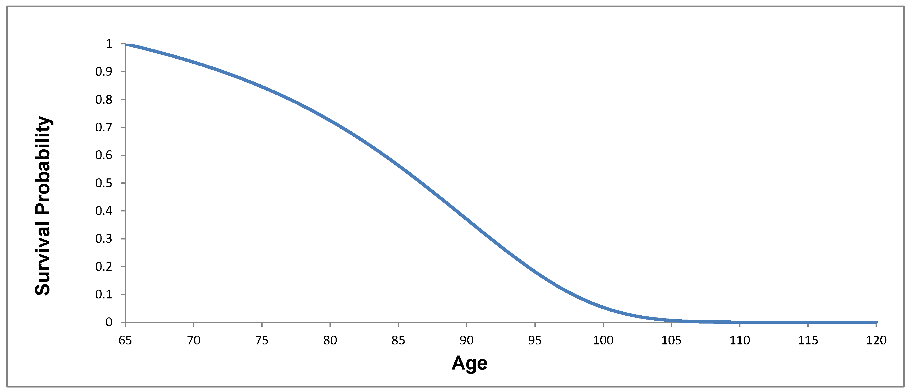
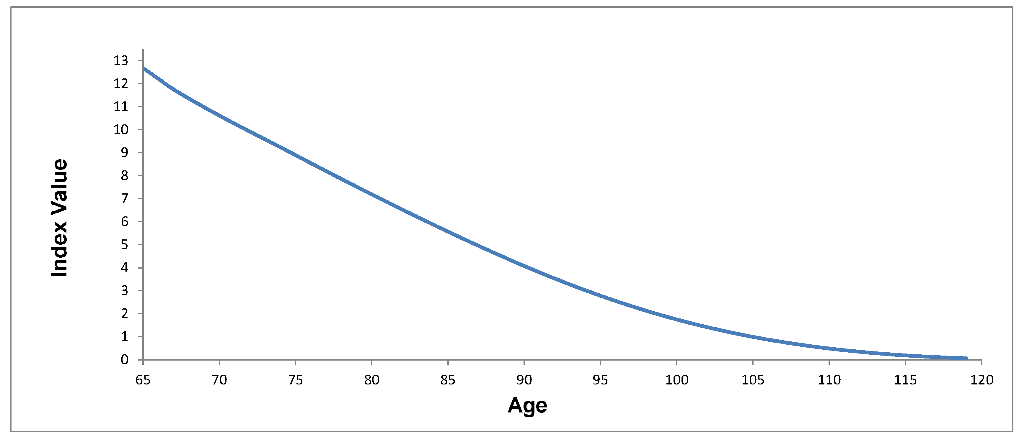
Based on the index, for a group of 65-year-old annuitants today, the annuity provider would require $P{V}_0$ today if it could fully hedge the longevity risk and interest rate risk. To determine the index, we use the mortality model parameters for the age 65 cohort, age 60 cohort and age 55 cohort. These three cohorts are chosen because the index values we will use will be based on initial ages from 55–65 at five-year intervals. We also project interest rates with the calibrated parameters of the interest rate model. With the estimated survival probabilities and interest rates, we are able to calculate the PV for each index point. Figure 9 shows the survival probabilities from the mortality model. Figure 10 shows the value index.

In Figure 10 $P{V}_0$ is equal to 12.66. This means that for each individual of the annuity portfolio, the annuity provider needs to invest 12.66 today per unit of income. The index takes a humped shape because it initially increases, then decreases. This is expected because the initial interest rate (observed rate) of each index point firstly decreases, then increases; therefore, the estimated discount factors follow the opposite direction. Although interest rates will be well hedged with the interest rate swaps, the realized survival probabilities will differ from the estimates, so the index is not risk-free even with the interest rate risk hedged and will reflect mortality variations.

The value-based index could be modified to only reflect mortality variations. In theory, this would be achieved by hedging the interest rate risk using a series of interest rate swaps (IRS) with the notional amount adjusted each year to account for mortality. At the beginning of each year of the hedging horizon, an IRS is initiated with a pre-determined notional amount and fixed rate. In the IRS, the annuity provider receives the fixed rate and pays the floating rate. Fixed rates are determined from the projected interest rates. Because the notional amount is invested at floating rates, if the realized number of survivors is exactly the same as estimated, the hedger will have exactly zero cash flow position at the end of the hedging horizon. For the first IRS entered at Time 0, the notional amount is simply $P{V}_0$. For the remaining hedging horizon, straightforward calculation shows that the notional amount at the beginning of year i is:

$$N_i=N_{i-1}(1+k_i)-n_i,\forall i\in [1,2,\dots ,\tau -1],$$

(27)

where $N_0=P{V}_0$. $n_i$ is the actual number of deaths, and $k_i$ is the fixed rate in the swap. This would produce an index that only fluctuated with mortality for the given cohort.

6.2. Hedge Efficiency

With the establishment of the value-based longevity index, we proceed to evaluate its efficiency in hedging value risk for a life annuity provider. We vary the size of a portfolio of annuitants who are Australian males aged 65 at present and evaluate the hedging effectiveness with the index level as the benchmark.

We consider two hedging instruments and compare their efficiencies. The first instrument is a swap in which the annuity provider pays the index value and receives the realized value. With such a swap, the annuity provider is able to transfer the systematic longevity risk and interest rate risk. However, the idiosyncratic longevity risk due to the differences between the portfolio and the population will remain.

The second hedging instrument is a survivor-forward (LLMA 2010). In the survivor-forward, or s-forward, the annuity provider pays the estimated population survival rate of cohort 65 and receives the realized population survival rate. Hence, the s-forward is only able to hedge the systematic longevity risk, but not the interest rate risk and the idiosyncratic longevity risk. Therefore, the hedge efficiency of the swap with the value index as the underlying relationshould compare favourably to the s-forward.

Our hedging methodology is standard. In order to generate idiosyncratic longevity risk for the portfolio, we follow Blackburn et al. (2017) and determine the random death time for each individual in the portfolio for the first time the mortality hazard rate exceeds $\varrho$, an exponential random variable with parameter one. For each simulation path m, we keep track of the number of accumulated deaths $d_i^m$ at the end of each year i ($i=1,2,\dots ,36$). If the initial number of annuitants of the portfolio is $n_0$, then the portfolio survival index at the end of each year i is:

$$\frac{n_0-d_i^m}{n_0},$$

(28)

When evaluating hedge efficiency, the existing literature tends to assume interest rates are constant or deterministic. As a result, the hedge efficiency is likely to be overestimated because interest rate risk is ignored (e.g., Coughlan et al. 2011; Blackburn and Sherris 2014). Suppose we want to hedge the value risk for a portfolio of male annuitants aged 65. We define the hedge efficiency as:

$$1-\frac{{\sigma }_h}{{\sigma }_u},$$

(29)

where ${\sigma }_h$ and ${\sigma }_u$ are respectively the standard deviation of the unexpected PV of the hedged position and the unhedged position.

If we simulate the mortality rates and interest rates with Monte Carlo, then for each path m, the unexpected value ($UV$) for the unhedged position is:

$$U{V}_u^m=P{V}_0-S{V}^m,$$

(30)

where $S{V}^m$ is the simulated PV of path m for the annuity portfolio allowing for both random future mortality and interest rates. It quantifies the unhedged annuity portfolio variations. These rates capture both aggregate and idiosyncratic mortality. The mortality model generates future stochastic mortality rates, and then for each mortality rate, the random number of deaths is generated.

For the hedged position with the index swap, the annuity provider enters a swap for the annuitant portfolio, and we assume the swap is collateralized and not subject to default risk. In the index swap, the hedger pays the fixed index value $P{V}_0$ and receives the realized value based on the index. Then, for each path m, the $UV$ is:

$$U{V}_{hswap}^m=SI{V}^m-S{V}^m,$$

(31)

where $SI{V}^m$ is the simulated PVof path m, for the age 65 cohort simulated population survival index with the calibrated mortality model parameters, reflecting only systematic longevity risk. The interest rate risk is hedged by the index swap.

For the hedged position with the s-forward, the $UV$ of each simulation path m is:

$$U{V}_{hforward}^m=P{V}_0-S{V}^m+SI{V}^m-{\overline{SIV}}^m,$$

(32)

where ${\overline{SIV}}^m$ is the simulated PV at projected population survival probabilities with random interest rates. In general, ${\overline{SIV}}^m\ne P{V}_0$ because in the s-forward, the interest rate risk is not hedged, only hedging the mortality rate.

Table 10. Hedge efficiency.

Portfolio Size	200	1000	100,00
Index Swap	12.60%	63.23%	95.73%
s-Forward	11.45%	52.31%	68.61%

shows the hedge efficiencies for the two proposed hedging instruments. We vary portfolio size to identify the effect of idiosyncratic longevity risk.

We see that for both instruments, hedge efficiency increases as portfolio size increases. However, the hedge efficiency improvement is more for the index swap than for the s-forward. For a group of 10,000 annuitants, the hedge efficiency is more than 95% for the swap, while less than 70% for the s-forward. This shows that the index swap is the more effective hedging instrument than the s-forward, particularly for a reasonably large portfolio. As discussed earlier in this section, these results are expected because only idiosyncratic longevity risk is retained with the value-based longevity index, which can be reduced by increasing the portfolio size. On the other hand, both idiosyncratic longevity risk and interest rate risk remain with the s-forward, and the latter cannot be reduced with larger portfolios.

7. Conclusions

Current longevity indices are based on the population mortality experience only. In this study, we propose a cohort-based value-index that reflects the present value of future obligations. This index captures both interest rate and mortality risk; as well as being relevant to individuals planning on purchasing an income in retirement, it is appropriate for benchmarking the hedging of both mortality risk and interest rate risk for a life annuity portfolio.

Based on the empirical data analyses, we develop a cohort-based stochastic mortality model that introduces age-dependent parameters and captures the main features of the historical cohort mortality data. The cohort correlation structures resulting from the model are more realistic. The fitting performance also improves for very old ages. We calibrate the one-factor Vasicek short rate model with Australian bond yields. The value index based on the projected survival probabilities and interest rates is the constructed for age 65. The value-based index takes into account both systematic longevity risk and interest rate risk. To illustrate the application of the index, we show how a swap with the index value as the underlying relationis more efficient in hedging the risk of a life annuity portfolio than the s-forward, which hedges systematic longevity risk only.

References

- Biffis, Enrico. 2005. Affine processes for dynamic mortality and actuarial valuations. Insurance: Mathematics and Economics 37: 443–68. [Google Scholar] [CrossRef]
- Blackburn, Craig, Katja Hanewald, Michael Sherris, and Annamaria Olivieri. 2017. Longevity risk management and shareholder value for a life annuity business. ASTIN Bulletin 47: 43–77. [Google Scholar] [CrossRef]
- Blackburn, Craig, and Michael Sherris. 2013. Consistent dynamic affine mortality models for longevity risk applications. Insurance: Mathematics and Economics 53: 64–73. [Google Scholar] [CrossRef]
- Blackburn, Craig, and Michael Sherris. 2014. Forward mortality modelling of multiple populations. Paper present at the 49th Actuarial Research Conference, Santa Barbara CA, USA, July, 13–16. Unpublished manuscript. [Google Scholar]
- Blake, David, Anja De Waegenaere, Richard McMinn, and Theo Nijman. 2009. Longevity risk and capital markets: The 2008–2009 update. Pensions Institute Discussion Paper (PI-0907). Insurance: Mathematics and Economics. [Google Scholar] [CrossRef] [Green Version]
- Bolder, David Jamieson. 2001. Affine Term-Structure Models: Theory and Implementation. Bank of Canada Working Paper 2001–1015. Ottawa: Bank of Canada, October. [Google Scholar]
- Brigo, Damiano, and Fabio Mercurio. 2006. Interest Rate Models: Theory and Practice, 2nd ed.Berlin: Springer-Verlag. [Google Scholar]
- Cairns, Andrew J., Kevin Dowd, David Blake, and Guy D. Coughlan. 2014. Longevity hedge effectiveness: A decomposition. Quantitative Finance 14: 217–35. [Google Scholar] [CrossRef] [Green Version]
- Cairns, Andrew J., and Delme J. Pritchard. 2001. Stability of descriptive models for the term structure of interest rates with application to German market data. British Actuarial Journal 7: 467–507. [Google Scholar] [CrossRef]
- Coughlan, Guy, David Epstein, Alen Ong, Amit Sinha, Javier Hevia-Portocarrero, Emily Gingrich, Marwa Khalaf-Allah, and Praveen Joseph. 2007. Lifemetrics: A Toolkit for Measuing and Managing Longevity and Mortality Risks, Technical report. Available online: www.lifemetrics.com (accessed on 17 January 2017).
- Coughlan, Guy, Marwa Khalaf-Allah, Yijing Ye, Sumit Kumar, Andrew Cairns, David Blake, and Andrew Cairns. 2011. Longevity hedging 101: A framework for longevity basis risk analysis and hedge effectiveness. North American Actuarial Journal 15: 150–76. [Google Scholar] [CrossRef] [Green Version]
- Cox, John C., Jonathan E. Ingersoll, and Stephen A. Ross. 1985. A theory of the term structure of interest rates. Econometrica 53: 385–407. [Google Scholar] [CrossRef]
- Dahl, Mikkel. 2004. Stochastic mortality in life insurance: Market reserves and mortality-linked insurance contracts. Insurance: Mathematics and Economics 35: 113–36. [Google Scholar] [CrossRef]
- DeutscheBörse. 2012. Deutsche Börse Xpect Club Vita Indices: Longevity Risk of Specific Pensioner Groups. Technical Report. Frankfurt: Deutsche Börse Market Data. [Google Scholar]
- Duffie, Darrell, and Rui Kan. 1996. A yield-factor model of interet rates. Mathematical Finance 6: 379–406. [Google Scholar] [CrossRef]
- Guimaraes, Marco Antonio. 2005. Half-Life in Mean Reversion Processes. Rio de Janeiro: Pontificia Universidade Catolica. [Google Scholar]
- Jevtic, Petar, Elisa Luciano, and Elena Vigna. 2013. Mortality surface by means of continuous time cohort models. Insurance: Mathematics and Economics 53: 122–33. [Google Scholar] [CrossRef]
- LLMA. 2010. Technical Note: The S-Forward. Washington: Life & Longevity Markets Association, October. [Google Scholar]
- Loeys, Jan, Nikolaos Panigirtzoglou, and Ruy M. Ribeiro. 2007. Longevity: A Market in the Making. Technical Report. New York: J.P. Moragn Securities Ltd. [Google Scholar]
- Luciano, Elisa, and Elena Vigna. 2005. Non Mean Reverting Affine Processes for Stochastic Mortality. ICER Working Paper Series (4/05); Boston: ICER. [Google Scholar]
- Luciano, Elisa, and Elena Vigna. 2008. Mortality risk via affine stochastic intensities: Calibration and empirical relevance. Belgian Actuarial Bulletin 8: 5–16. [Google Scholar]
- Ngai, Andrew, and Michael Sherris. 2011. Longevity risk management for life and variable annuities: The effectiveness of static hedging using longevity bonds and derivatives. Insurance: Mathematics and Economics 49: 100–14. [Google Scholar] [CrossRef]
- Njenga, Carolyn N., and Sherris Michael. 2011. Longevity risk and the econometric analysis of mortality trends and volatility. Asia-Pacific Journal of Risk and Insurance 5: 22–73. [Google Scholar] [CrossRef]
- Schrager, David F. 2006. Affine stochastic mortality. Insurance: Mathematics and Economics 38: 81–97. [Google Scholar] [CrossRef]
- Sherris, Michael. 2009. AIPAR Longevity Index. Sydney: Australian Institute for Population Ageing Research, September. [Google Scholar]
- Sherris, Michael, and Samuel Wills. 2008. Financial innovation and the hedging of longevity risk. Asia-Pacific Journal of Risk and Insurance 3: 1–14. [Google Scholar] [CrossRef]
- Vasicek, Oldrich. 1977. An equilibrium characterization of the term structure. Journal of Financial Economics 5: 177–88. [Google Scholar] [CrossRef]
- Wadsworth, Michael. 2005. The Pension Annuity Market: Further Research Into Supply and Constraints. Technical Report. London: Association of British Insurers. [Google Scholar]