Preliminary Investigations for Better Monitoring: Learning in Repeated Insurance Audits

Abstract

Audit mechanisms frequently take place in the context of repeated relationships between auditor and auditee. This paper focuses attention on the insurance fraud problem in a setting where insurers repeatedly verify claims satisfied by service providers (e.g., affiliated car repairers or members of managed care networks). We highlight a learning bias that leads insurers to over-audit service providers at the beginning of their relationship. The paper builds a bridge between the literature on optimal audit in insurance and the exploitation/exploration trade-off in multi-armed bandit problems.

1. Introduction

Claim fraud represents a serious threat to insurance markets: by artificially inflating the frequency and the cost of reported losses, defrauders lead to higher insurance premiums and they contribute to jeopardizing the efficiency of risk sharing mechanisms. Besides the free-riding problem that it poses, large scale fraud may even endanger the sustainability of the insurance markets that are prone to fraud.

Insurance claim fraud is sometimes referred to as a form of ex-post moral hazard in that it occurs after an (alleged) accident—for example when policyholders build up their claim or when they announce accidents that never actually happened. It essentially differs from ex-ante moral hazard through the associated timing (before/after the accident) and the modus operandi of addressing these inefficiencies: while principals tend to rely on a contract design approach to distort the agent’s incentives in an ex-ante context (without being able to monitor the agent’s effort), the ex-post situation is usually addressed through costly auditing in order to check what actually occurred.

The economic literature has mainly examined these issues through the lens of the costly state verification approach, whose foundations were laid by the seminal papers of Townsend (1979) and Gale and Hellwig (1985). Within this setting, it is assumed that the insurer can verify the true value of claims by incurring an audit cost.1 The audit may be either deterministic, random or guided by signals perceived by the insurer. In particular, Mookherjee and Png (1989) establish that random auditing dominates deterministic auditing, while Dionne et al. (2008) build a scoring methodology to show how audits are triggered by signals observed by the insurer. In one way or another, an optimal claim monitoring strategy achieves a trade-off between the additional costs of more frequent audits and the advantages of a more efficient fraud detection. The deterrence effect highlighted by Dionne et al. (2008) is an example of such an advantage: they consider a setting where more frequent audits reduce the frequency of fraud, and they show that some individually unprofitable audits should be performed because of this deterrence effect.

Audits may also play an important role in gathering evidence about the auditee (e.g., does he seem to have a penchant for dishonest behavior?), information that may be useful at later stages. Indeed, claimants (or service providers with whom they collude) may have some intrinsic and hard to observe characteristics that affect their propensity to defraud. Audits may help the insurer to mitigate this informational asymmetry about claimants’ type.2

The learning dimension is particularly relevant when it comes to repeated audits. Consider, for instance, the health insurance fraud case when there is a third party involved beside the insurer and the policyholders. Health service providers (doctors, opticians, pharmacists, etc.) play a central role since collusion between providers and policyholders is usually a necessary condition for fraud to take place. Furthermore, health care providers interact on a regular basis with the insurer, as they provide services to many policyholders and during several periods. Because of this repeated interaction, health insurers’ anti-fraud efforts often focus on service providers as much as on policyholders. The same logic applies to property insurance, when insurers interact with car repairers or construction companies, sometimes within a network of affiliated service providers.

The purpose of the present paper is to investigate how such repeated interactions affect the optimal audit strategy. We will show that the insurer may find it optimal to perform unprofitable audits because of a learning effect. In short, auditing is a way to gather information that can be used at later stages of the auditor–auditee interaction. This learning dimension may lead the insurer to perform audits beyond what would be optimal from a purely instantaneous standpoint.

To highlight this effect, we will rely on a simple model with two types of service providers (honest and dishonest) and where the likelihood of submitting an invalid claim is exogenous and type-dependent. Thus, we abstain from analyzing the strategic interaction between the insurer and policyholders. We focus attention on the role of service providers as mandatory intermediaries who certify claims, without examining the collusion process between providers and claimants.3 Dishonest providers may certify invalid claims on purpose, while honest providers may only do it unintentionally. The insurer has beliefs about the type of each service provider and his decision consists of choosing the probability with which he audits each provider over the course of two consecutive periods. Auditing a claim allows the insurer to discover whether it is valid or invalid, but, in the latter case, it does not reveal if the misbehavior was done on purpose or unintentionally. Auditing a claim allows the insurer to update his belief about the type of the service provider.

We find that, in the first period, the insurer has an incentive to perform some unprofitable audits, in order to improve his information about the service providers’ type, and this additional information will allow him to more efficiently focus his auditing strategy at the second period. Ultimately, deviating from a strategy that would be guided by instantaneous expected gains proves to be profitable. It corresponds to insisting on preliminary investigations early in the relationship to better monitor the agents later on.

This conclusion reveals an exploration/exploitation dilemma analogous to the multi-armed bandit problem in machine learning.4 In this approach, a player is repeatedly facing a slot machine with multiple arms. He must choose an arm at each period, each arm providing a random payoff with an imperfectly known stationary distribution. The player faces a trade-off between playing the most profitable arm according to early beliefs, and playing different arms in order to refine his beliefs. Exploring new arms induces an opportunity cost of not exploiting the arm that is the most profitable according to the current information, but this may allow the player to discover that other arms are in fact more profitable. Similarly, in our model, by trading current revenue for information, the better informed insurer gets a higher future payoff that compensates the initial loss.

The rest of the paper is organized as follows. In Section 2, as a preliminary stage, we consider a single period model where audits are not repeated and we characterize the corresponding optimal auditing strategy. In Section 3, we extend our model to account for repeated audits. We exhibit the competing roles of auditing as sources of revenue and information, and we define the insurer’s dynamic optimization problem that will be solved by backward induction. Hence, we start by characterizing how available information is used at the second period and, in a second stage, we deduce how the first period audit should be performed. We show that the learning effect leads the insurer to audit more at the beginning of the relationship, with the magnitude depending on the informativeness of the audit and on the degree of short-sightedness of the insurer. In Section 2 and Section 3, we restrain ourselves to a simple model where all claims have the same value. Section 4 extends our results to a more general setting with variable claim values. The final section concludes. Proofs are in the Appendix A.

2. Single Period Auditing

2.1. Setting

Let us start by considering an insurer who interacts with a population of service providers (SPs) during a single period. SPs are mandatory intermediaries between insurer and insured. In particular, they certify the claims filed by policyholders, which means that they attest that the claims actually correspond to the value of the services paid by the policyholders following the event covered by the insurance policy. Each SP transmits exactly one claim with a value normalized to 1 to the insurer, with the claim being either valid or invalid. Invalid claims should not lead to insurance payments. They may be transmitted either in good faith (for instance because the SP makes an error due to imperfect information about the circumstances of the loss) or in bad faith with the intention of defrauding.

SPs are heterogeneous when it comes to their propensity to transmit invalid claims. There are many possible determinants of this propensity, among which is the sense of moral values, which is negatively correlated with the propensity to defraud or the ability to build complex defrauding schemes.5 Hereafter, we consider that each SP may be either honest (H) or dishonest (D). Honest SPs only transmit invalid claims by error (they are always in good faith), while dishonest SPs may transmit invalid claims either by error or intentionally (they may be in bad faith). Hence, a type H is less likely to transmit invalid claims than a type D. We include this aspect by defining probabilities $\mathbb{P}(Inv|H)=p_H$ and $\mathbb{P}(Inv|D)=p_D$ of submitting an invalid claim by type H and type D, respectively, such that $p_H<p_D$.

There is a continuum of SPs with mass 1 and the insurer has initial belief $\pi \in [0,1]$ for each SP that represents the a priori probability that the SP is of type D. The prior $\pi$ is distributed in $[0,1]$ with density $f(\pi )$ and cumulative distribution function (c.d.f.) $F(\pi )$ in the population of SPs. While we consider this prior as given, we may consider that it has been induced by signals (including the outcome of audits) that have been previously perceived by the insurer about each SP. These beliefs may be biased or not among SPs, i.e., the expected value ${\int }_0^1\pi f(\pi )d\pi$ may or may not be equal to the true proportion of dishonest SPs in the continuum.

Each claim may be audited and, in that case, the insurer observes whether it is valid or invalid. The audit is costly and represents the fundamental constraint that the insurer faces when it comes to choosing audit targets. It costs c to investigate a claim, with $p_H<c<p_D$.

Claims found to be invalid are not paid, inducing a net proceed of $1-c$. No penalty is paid to the insurer by SPs whose invalid claims are detected by the audit. Hence, auditing a claim is profitable (in expected terms) only when it has been certified by a dishonest SP. From the insurer’s point of view, an SP with prior $\pi$ transmits invalid claims with probability $\overline{p}(\pi )=p_D\pi +p_H(1-\pi )$ and the corresponding expected net proceed of auditing is $\overline{p}(\pi )-c$.

2.2. Auditing Strategy, Objective Function and Optimization Problem

For each SP, the insurer must decide whether an audit will be performed or not. We define an auditing strategy as a function $x(·):[0,1]\to [0,1]$ that assigns a probability $x(\pi )$ of being audited to each SP with belief $\pi$. For a given auditing strategy, the net expected proceed of audits is written as

$$\Omega (x(·))={\int }_0^1\left[\overline{p}(\pi )-c\right]x(\pi )f(\pi )d\pi .$$

The optimization problem of the insurer is written as

$$\begin{array}{cc}\hfill \underset{x(·)}{max}& \Omega (x(·))\hfill \\ \hfill s.t.& 0\le x(\pi )\le 1\forall \pi \in [0,1].\hfill \end{array}$$

Lemma 1.

The single period optimal auditing strategy $x^{*}(\pi )$ consists in auditing all claims transmitted by SPs with associated beliefs $\pi \ge {\pi }^{*}$ and not auditing claims when $\pi <{\pi }^{*}$, i.e.,

$$\begin{array}{c}\hfill x^{*}(\pi )=\left\{\begin{array}{c}1if\pi \in [{\pi }^{*},1]\hfill \\ 0if\pi \in [0,{\pi }^{*})\hfill \end{array}\right\}={\mathbb{1}}_{\{\pi \ge {\pi }^{*}\}},\end{array}$$

where the threshold ${\pi }^{*}$ is

$${\pi }^{*}=\frac{c-p_H}{p_D-p_H}\mathit{with}\overline{p}({\pi }^{*})-c=0.$$

Lemma 1 is unsurprising: one should only perform audits that are individually profitable, which amounts to focusing audits on SPs with $\pi$ such that $\overline{p}(\pi )-c\ge 0$.

3. Two-Period Auditing: The Learning Effect

Because SPs take care of many policyholders, they repeatedly interact with the insurer. For the sake of simplicity, we assume that this interaction takes place during two consecutive periods $i=0,1$. There are different beliefs at the beginning of each period and the insurer’s strategy is based on these beliefs. From now on, variables of interest will be indexed by the corresponding periods ${({\pi }_i,x_i,{\Omega }_i)}_{i\in \{0,1\}}$. The insurer’s inter-temporal objective function depends on both period specific objective functions ${\Omega }_0$ and ${\Omega }_1$, the latter being weighted by $\gamma >0$.6 His optimization problem is written as

$$\begin{array}{c}\underset{x_0(·),x_1(·)}{max}{\Omega }_0+\gamma {\mathbb{E}}_0[{\Omega }_1],\hfill \\ s.t.0\le x_0({\pi }_0)\le 1\forall {\pi }_0\in [0,1],\hfill \\ s.t.0\le x_1({\pi }_1)\le 1\forall {\pi }_1\in [0,1],\hfill \end{array}$$

where ${\mathbb{E}}_0$ corresponds to the expected value operator at the beginning of period 0, i.e., before performing audits during this period.

3.1. Auditing as a Source of Information

Period 0 audits allow the insurer to update his belief at the beginning of period 1. Depending on whether an audit has been performed and, if it has been, whether the claim was valid or invalid (Val and Inv, respectively), the updated beliefs ${\tilde{\pi }}_1$ are deduced from initial beliefs ${\pi }_0$ through Bayes’ Law:

$$\widetilde{{\pi }_1}=\left\{\begin{array}{c}\mathbb{P}(D|audit,Inv)=A({\pi }_0)=\frac{p_D{\pi }_0}{\overline{p}({\pi }_0)},\hfill \\ \mathbb{P}(D|audit,Val)=B({\pi }_0)=\frac{(1-p_D){\pi }_0}{1-\overline{p}({\pi }_0)},\hfill \\ \mathbb{P}(D|noaudit)={\pi }_0,\hfill \end{array}\right.$$

(1)

with

$$\begin{array}{c}B({\pi }_0)<{\pi }_0<A({\pi }_0),\hfill \\ A^{\prime }>0,A^{″}<0,\hfill \\ B^{\prime }>0,B^{″}>0.\hfill \end{array}$$

Hence, $A({\pi }_0)$ and $B({\pi }_0)$ are the probabilities that the SP is dishonest if a period 0 audit revealed that the claim was invalid or valid, respectively. In particular, an invalid claim detected by audit leads the insurer to increase his beliefs that the SP is dishonest, i.e., $A({\pi }_0)>{\pi }_0$, and it is the other way around if an audit reveals that the claim was valid, i.e., $B({\pi }_0)<{\pi }_0$. Of course, beliefs are unchanged if there is no audit.

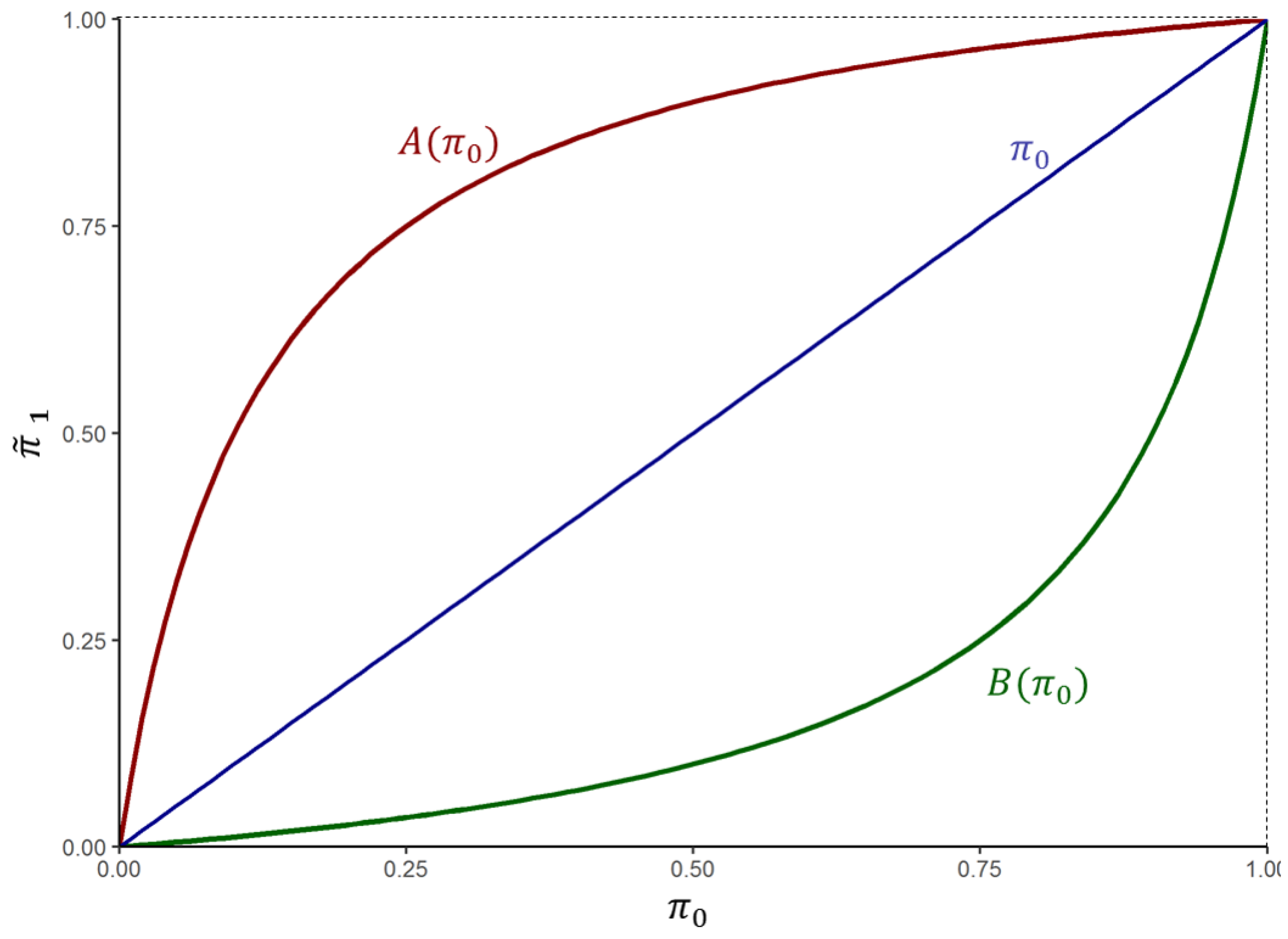
For illustrative purposes, Figure 1 and Figure 2 describe the degree of informativeness of an audit as a function of parameters $p_H$ and $p_D$. In Figure 1, the graphs of functions $A(·)$ and $B(·)$ are symmetric on each side of the ${45}^{\circ }$ line. This is due to the specific condition $p_H+p_D=1$. Maintaining this assumption, Figure 2a shows that bringing $p_H$ and $p_D$ closer makes both learning curves less concave/convex and closer to the ${45}^{\circ }$ line, underlining the fact that the audit is less informative in this case. Figure 2b,c illustrate the extreme case where the audit is, respectively, totally informative ($p_H=0$ and $p_D=1$) and not informative at all ($p_H=p_D$, both types behave the same way). Relaxing the $p_H+p_D=1$ assumption, Figure 2d–f exemplify the asymmetry of informativeness between invalidity and validity of a claim: in Figure 2d, both probabilities of defrauding are rather low, so stumbling upon a valid claim does not say much, while finding a claim to be invalid induces a stronger change in the belief. The opposite happens in Figure 2e where both types defraud often, with the validity status becoming more informative.

This aspect of auditing suggests some influence of period 0 auditing outcomes on period 1 auditing decisions. The information revealed at period 0 may lead to an expected efficiency gain at period 1. To express this idea, let us denote $\omega ({\pi }_1,x_1)=\left[\overline{p}({\pi }_1)-c\right]x_1$ the expected gain of an audit performed at period 1 with probability $x_1$ under belief ${\pi }_1$.

Proposition 1.

The optimal period 1 optimal audit strategy $x_1^{*}(·)$ is such that

$$\begin{array}{c}\hfill {\mathbb{E}}_0[\omega ({\tilde{\pi }}_1,x_1^{*}({\tilde{\pi }}_1))|{\pi }_0,x_0({\pi }_0)]\ge \omega ({\pi }_0,x_1^{*}({\pi }_0))\forall {\pi }_0\in [0,1]\end{array}$$

with a strict inequality if ${\pi }_1\in [0,1]$ exists such that $x_1^{*}({\pi }_1)\ne x_1^{*}({\pi }_0)$ and $\mathbb{P}({\tilde{\pi }}_1={\pi }_1|{\pi }_0)>0$.

Proposition 1 implies that period 0 auditing increases the insurer’s period 1 expected payoff if it affects the period 1 auditing strategy: its informational value translates into an increase in period 1 net proceeds besides its period 0 income maximization value.

Let ${\tilde{\pi }}_1$ be the updated belief. This is a random variable defined by Equation (1) whose distribution depends on initial beliefs ${\pi }_0$ and on the period 0 auditing probability $x_0({\pi }_0)$.

3.2. Inter-Temporal Optimization Problem

Period 0 expected auditing profit is written as

$${\Omega }_0(x_0(·))={\int }_0^1\left[\overline{p}({\pi }_0)-c\right]x_0({\pi }_0)f_0({\pi }_0)d{\pi }_0,$$

where $f_0({\pi }_0)$ is the density of prior beliefs.

The updating process corresponds to a mapping of period 0 beliefs into period 1 beliefs, thus changing the latter’s distribution depending on the chosen period 0 strategy. Let $f_1(·)$ be the density of period 1 updated beliefs. It depends on period 0 auditing strategy and then it is written as $f_1({\pi }_1|x_0(·))$. Period 1 expected auditing profit is written as

$${\Omega }_1(x_0(·),x_1(·))={\int }_0^1\left[\overline{p}({\pi }_1)-c\right]x_1({\pi }_1)f_1({\pi }_1|x_0(.))d{\pi }_1.$$

The inter-temporal optimal auditing strategy of the insurer can now be characterized by backward induction. At period 1, the insurer follows the optimal single period strategy $x_1^{*}(·)$ characterized by Lemma 1. Hence, the optimal period 1 expected net proceed of auditing ${\Omega }_1^{*}(x_0(·))={\Omega }_1(x_0(·),x_1^{*}(·))$ is written as

$$\begin{array}{cc}\hfill {\Omega }_1^{*}(x_0(·))& ={\int }_0^1\left[\overline{p}({\pi }_1)-c\right]{\mathbb{1}}_{\{\pi \ge {\pi }^{*}\}}{f}_1({\pi }_1|x_0(.))d{\pi }_1\hfill \\ & ={\int }_{{\pi }^{*}}^1\left[\overline{p}({\pi }_1)-c\right]f_1({\pi }_1|x_0(.))d{\pi }_1.\hfill \end{array}$$

Given this period 1 optimal strategy, the period 0 optimal strategy $x_0^{*}(·)$ is an optimal solution to

$$\begin{array}{c}\underset{x_0(·)}{max}{\Omega }_0(x_0(·))+\gamma {\mathbb{E}}_0[{\Omega }_1^{*}(x_0(·))]\hfill \\ s.t.0\le x_0({\pi }_0)\le 1\forall {\pi }_0\in [0,1].\hfill \end{array}$$

3.3. Effect of Period 0 Audit on the Audit Decision in Period 1

In order to show how period 0 audit affects the decision to audit at period 1, let us define ${\pi }_a$ and ${\pi }_b$ by

$$\begin{array}{cc}A({\pi }_a)={\pi }^{*},\hfill & {\pi }_a=\frac{{\pi }^{*}{p}_H}{{\pi }^{*}{p}_H+(1-{\pi }^{*})p_D},\hfill \\ B({\pi }_b)={\pi }^{*},\hfill & {\pi }_b=\frac{{\pi }^{*}(1-p_H)}{{\pi }^{*}(1-p_H)+(1-{\pi }^{*})(1-p_D)}.\hfill \end{array}$$

One easily checks that

$$0<{\pi }_a<{\pi }^{*}<{\pi }_b<1.$$

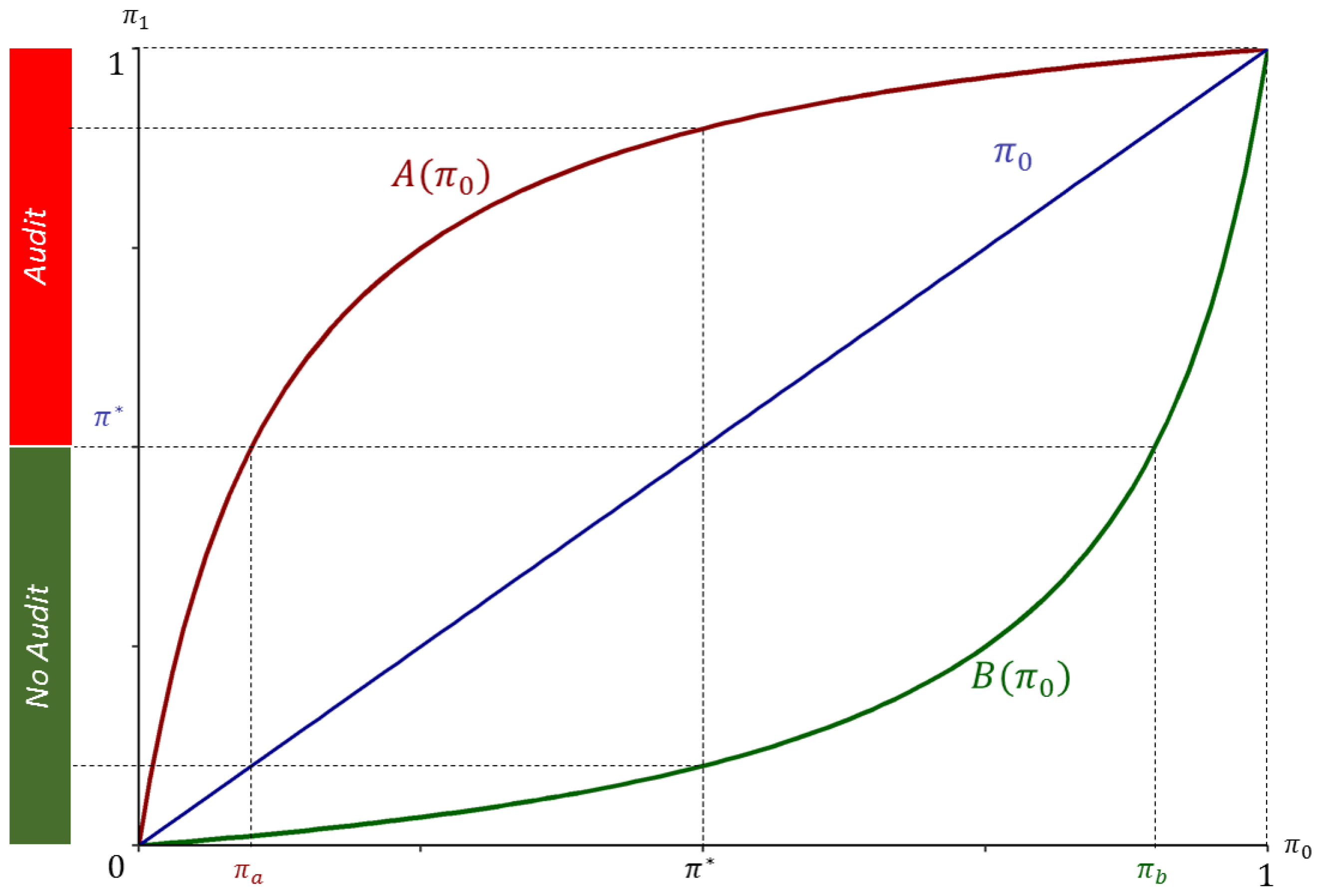
We have $A(\pi )\ge {\pi }^{*}$ if and only if $\pi \ge {\pi }_a$ and $B(\pi )\ge {\pi }^{*}$ if and only if $\pi \ge {\pi }_b$. Hence, ${\pi }_a$ is the lowest belief such that, if found invalid at period 0, the SP will be audited at period 1 and ${\pi }_b$ is the highest belief such that, if found valid at period 0, the SP will be not be audited at period 1.

These thresholds lead us to Lemma 2 in which we express the probability of auditing at period 1 as a function of the period 0 belief and auditing outcomes.

Lemma 2.

The effect of period 0 audit on the audit decision $x_1$ at period 1 is characterized by

Table 1. Period 1 audit decision $x_1$ as a function of period 0 beliefs and audit outcomes.

${\mathit{\pi }}_0\in$	$[0,{\mathit{\pi }}_{\mathit{a}})$	$[{\mathit{\pi }}_{\mathit{a}},{\mathit{\pi }}^{*})$	$[{\mathit{\pi }}^{*},{\mathit{\pi }}_{\mathit{b}})$	$[{\mathit{\pi }}_{\mathit{b}},1]$
Audit and Valid	0	0	0	1
No Audit	0	0	1	1
Audit and Invalid	0	1	1	1

.

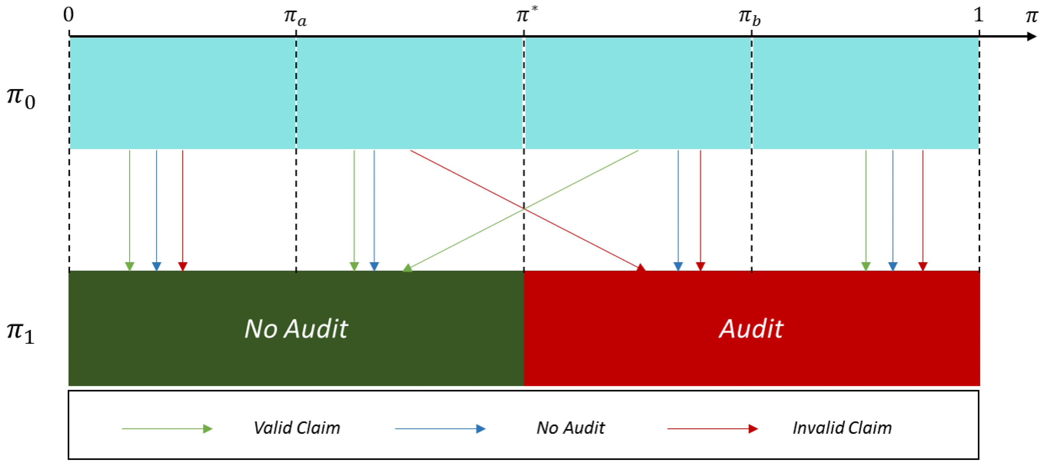
Figure 3 and Figure 4 illustrate this relationship between the outcomes of the period 0 audit and the obtained posteriors.

Lemma 2 directly yields the probability of being audited at period 1 conditionally on ${\pi }_0$ and $x_0({\pi }_0)$. This is written as

$$\begin{array}{cc}\mathbb{P}({\pi }_1\ge {\pi }^{*}|{\pi }_0\in [0,{\pi }_a))\hfill & =0,\hfill \\ \mathbb{P}({\pi }_1\ge {\pi }^{*}|{\pi }_0\in [{\pi }_a,{\pi }^{*}))\hfill & =\overline{p}({\pi }_0)x_0({\pi }_0),\hfill \\ \mathbb{P}({\pi }_1\ge {\pi }^{*}|{\pi }_0\in [{\pi }^{*},{\pi }_b))\hfill & =\overline{p}({\pi }_0)x_0({\pi }_0)+1-x_0({\pi }_0),\hfill \\ \mathbb{P}({\pi }_1\ge {\pi }^{*}|{\pi }_0\in [{\pi }_b,1])\hfill & =\overline{p}({\pi }_0)x_0({\pi }_0)+1-x_0({\pi }_0)+(1-\overline{p}({\pi }_0))x_0({\pi }_0)=1.\hfill \end{array}$$

For instance, when ${\pi }_0\in [{\pi }^{*},{\pi }_b)$, there will be an audit at period 1 either if, at period 0, an audit revealed an invalid claim or if there was no audit, which occurs with probability $\overline{p}({\pi }_0)x_0({\pi }_0)$ and $1-x_0({\pi }_0),$ respectively. The other cases can be interpreted similarly.

Lemma 3.

The inter-temporal objective function can be rewritten as

$$\begin{array}{cc}\hfill {\Omega }_0(x_0(·))+\gamma {\mathbb{E}}_0[{\Omega }_1^{*}(x_0(·))]& ={\int }_0^1\left[C({\pi }_0)+K({\pi }_0)x_0({\pi }_0)\right]f_0({\pi }_0)d{\pi }_0,\hfill \end{array}$$

where functions $C(·)$ and $H(·)$ are defined in

Table 2. Definition of $C(·)$ and $H(·)$.

${\pi }_0$	$C({\pi }_0)$	$H({\pi }_0)$
$[0,{\pi }_a)$	0	0
$[{\pi }_a,{\pi }^{*})$	0	$p_D^2{\pi }_0+p_H^2(1-{\pi }_0)-\overline{p}({\pi }_0)c$
$[{\pi }^{*},{\pi }_b)$	$\gamma \left[\overline{p}({\pi }_0)-c\right]$	$p_D^2{\pi }_0+p_H^2(1-{\pi }_0)-\overline{p}({\pi }_0)c-[\overline{p}({\pi }_0)-c]$
$[{\pi }_b,1]$	$\gamma \left[\overline{p}({\pi }_0)-c\right]$	0

and $K({\pi }_0)=\overline{p}({\pi }_0)-c+\gamma H({\pi }_0)$. In particular, $K({\pi }_0)$ is a continuous piecewise linear function such that

$$\begin{array}{c}K({\pi }_0)<0\mathit{if}{\pi }_0\le {\pi }_{a}andK({\pi }_0)>0\mathit{if}{\pi }_0>{\pi }^{*},\hfill \\ K({\pi }_0)=\overline{p}({\pi }_0)-c\mathit{for}{\pi }_0\in (0,{\pi }_a)\cup ({\pi }_b,1),\hfill \\ K({\pi }_0)>\overline{p}({\pi }_0)-c\mathit{for}{\pi }_0\in ({\pi }_a,{\pi }_b).\hfill \end{array}$$

Lemma 3 decomposes the inter-temporal objective function into components that make explicit the impact of $x_0(·)$ on current and future audit proceeds. $C({\pi }_0)$ represents the proceeds of period 1 audits when the SP is not audited at period 0, and thus this term is not affected by $x_0({\pi }_0)$. Beliefs ${\pi }_0$ in $[0,{\pi }_a)$ and $[{\pi }_a,{\pi }^{*})$ are smaller than ${\pi }^{*}$, and, thus, if the corresponding SPs are not audited at period 0, neither will they be at period 1. Hence, any benefit/loss from these beliefs is necessarily the consequence of being audited at period 0, which gives $C({\pi }_0)=0$. This is different for beliefs in $[{\pi }^{*},{\pi }_b)$ and $[{\pi }_b,1]$ because they correspond to cases where initial beliefs ${\pi }_0$ are higher than ${\pi }^{*}$. Consequently, the SPs will be audited at period 1 and there are some proceeds from period 1 that do not depend on $x_0(·)$, hence the presence of $\gamma$ in $C(·)$.

$K({\pi }_0)$ represents the proceeds over the two periods that are affected by period 0 audit. $\overline{p}({\pi }_0)-c$ in $K({\pi }_0)$ represents the period 0 proceeds resulting from being audited at that period, while $H({\pi }_0)$ corresponds to the period 1 proceeds that are affected by period 0 audits through the belief updating process. For instance, an SP with ${\pi }_0\in [{\pi }_a,{\pi }^{*})$ will be audited at period 1 if an audit revealed an invalid claim at period 0 (because ${\pi }_1\ge {\pi }^{*}$ in that case) and the term $p_D^2{\pi }_0+p_H^2(1-{\pi }_0)-\overline{p}({\pi }_0)c$ corresponds to the expected net proceeds. $H({\pi }_0)=0$ in $[0,{\pi }_a)$ and $[{\pi }_b,1]$, although for different reasons: in $[0,{\pi }_a)$, regardless of the outcome of the audit, updated beliefs will remain below ${\pi }^{*}$ and will never be audited at period 1, while, in $[{\pi }_b,1]$, whatever happens at period 0, all beliefs remain above ${\pi }^{*}$ and the claim will always be audited at period 1. Function $K({\pi }_0)$ is illustrated in Figure 5.

3.4. Inter-Temporal Optimal Auditing Strategy

Proposition 2.

An optimal period 0 strategy $x_0^{*}(·)$ is characterized by ${\pi }^{**}\in ({\pi }_a,{\pi }^{*})$ such that

$$\begin{array}{c}{x}_0^{*}({\pi }_0)=0\mathit{if}{\pi }_0\in [0,{\pi }^{**}),\hfill \\ x_0^{*}({\pi }_0)\in [0,1]\mathit{if}{\pi }_0={\pi }^{**},\hfill \\ x_0^{*}({\pi }_0)=1\mathit{if}{\pi }_0\in ({\pi }^{**},1].\hfill \end{array}$$

The threshold ${\pi }^{**}$ is given by

$${\pi }^{**}={\pi }^{*}\frac{1+\gamma p_H}{1+\gamma p_H+\gamma (p_D-c)}<{\pi }^{*},$$

and is such that

$$K({\pi }^{**})=0\mathit{and}\overline{p}({\pi }_0)-c<0\forall {\pi }_0\in [{\pi }^{**},{\pi }^{*}).$$

(2)

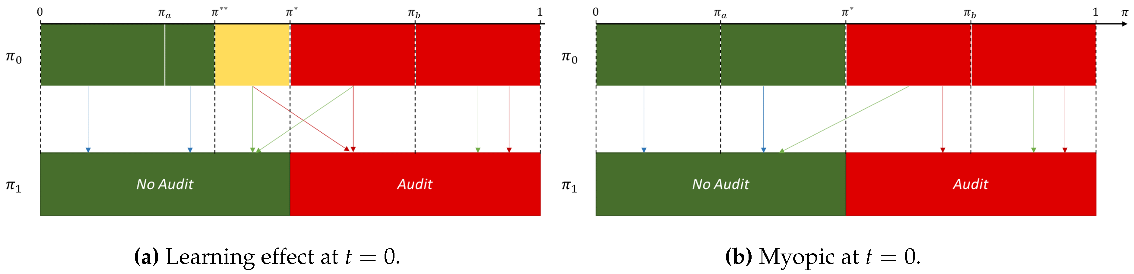
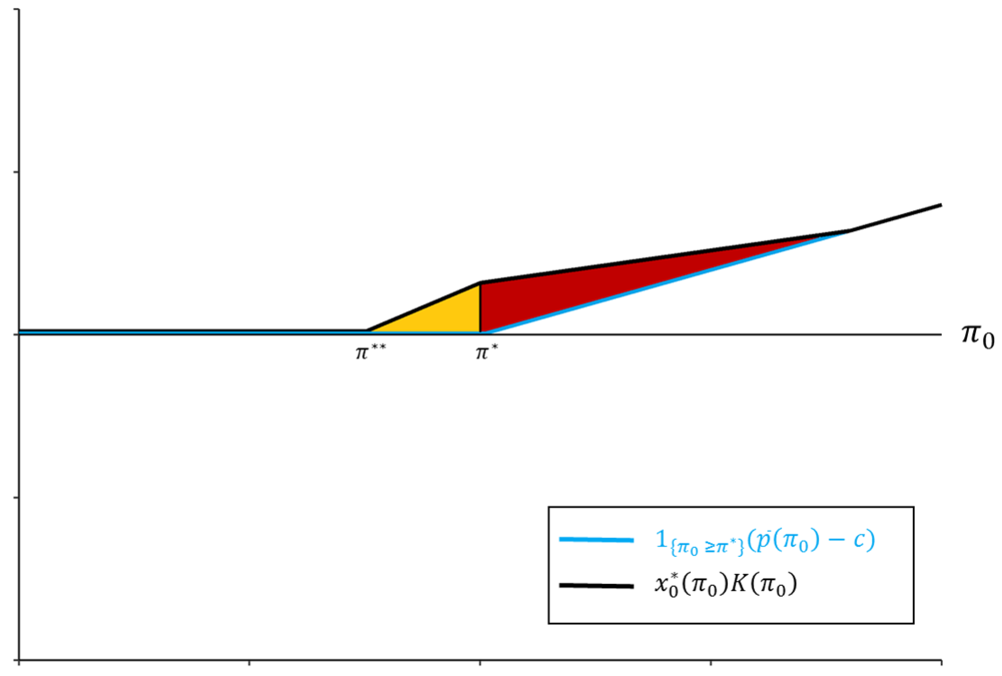
Proposition 2 shows that, accounting for the impact of period 0 auditing on period 1, posterior beliefs lead the insurer to audit a higher number of SPs at period 0 than in the instantaneous audit problem analyzed in Section 2. The belief threshold above which claims should be audited is now ${\pi }^{**}$ instead ${\pi }^{*}$, with ${\pi }^{**}<{\pi }^{*}$. An interesting aspect is that these additional auditees ${\pi }_0\in [{\pi }^{**},{\pi }^{*})$ are such that the corresponding individual expect net proceeds of audit are negative (Equation (2)): in other words, in spite of the negative impact on period 0 audit proceeds, the information gathered generates enough (discounted) profit at period 1 to compensate for this initial loss. Figure 6 illustrates this deviation from the single period myopic auditing and Figure 7 shows in orange the additional period 1 positive net proceeds $\gamma \int H({\pi }_0)f_0({\pi }_0)d{\pi }_0$ that come from auditing down to ${\pi }^{**}$.7

The extent of the informational value of auditing is illustrated by the comparative statics properties of ${\pi }^{**}$. If $\gamma =0$, i.e., if the insurer at time 0 does not care about period 1, then ${\pi }^{**}={\pi }^{*}$ since the informational value of auditing at $t=0$ serves no purpose. If $\gamma \to +\infty$, i.e., if the insurer only cares about period 1 profit, then ${\pi }^{**}\to {\pi }_a$ and he seeks to get the maximum information from period 0. Of course, there is no point in having ${\pi }^{**}$ lower than ${\pi }_a$ as the additional information would not be useful at period 1. The new auditing limit, like the myopic one, also depends on c: if $c=p_H$, then ${\pi }^{**}={\pi }^{*}=0$ and, if $c=p_D,$ then ${\pi }^{**}={\pi }^{*}=1$, as in both cases there is no more trade-off between information and revenue. Finally, if we write $c=\alpha p_D+(1-\alpha )p_H$ with $\alpha \in (0,1)$, then ${\pi }^{*}=\alpha$ and ${\pi }^{**}\to {\pi }^{*}$ when $p_D⟶p_H$. When $p_D$ comes closer to $p_H$, the separating power of the audit decreases until it becomes uninformative, and, at the limit $p_D=p_H$, there is no more distinction between types D and H.

4. Variable Claim Value

A large part of the economic analysis of insurance fraud has focused attention on optimal auditing strategies when policyholders may file smaller or larger claims, and, on the way, the insurer’s audit strategy depends on the size of the claim.8 Let us consider how this approach may be affected by the learning mechanism.

4.1. Deterministic Value

As a preliminary step, let us consider the case where the size of all claims takes some arbitrary value $\ell \in {\mathbb{R}}^{+}$. This size is still fixed, but not necessarily equal to 1. The belief threshold ${\pi }^{*}$ now depends on ℓ and is defined by

$$\begin{array}{cc}{\pi }^{*}=1\hfill & \mathrm{if}\ell \le \frac{c}{p_D},\hfill \\ \overline{p}({\pi }^{*})\ell -c=0\hfill & \mathrm{if}\frac{c}{p_D}<\ell <\frac{c}{p_H},\hfill \\ {\pi }^{*}=0\hfill & \mathrm{if}\frac{c}{p_H}\le \ell .\hfill \end{array}$$

Therefore,

$$\begin{array}{cc}\hfill {\pi }^{*}(\ell )& =max\left\{0,min\left\{1,\frac{c/\ell -p_H}{p_D-p_H}\right\}\right\}.\hfill \end{array}$$

Equivalently, we may define a threshold ${\ell }^{*}$ for the claim size

$$\begin{array}{c}\hfill {\ell }^{*}(\pi )=\frac{c}{p_H+(p_D-p_H)\pi }=\frac{c}{\overline{p}(\pi )}\forall \pi \in [0,1],\end{array}$$

and, for beliefs $\pi$, auditing is profitable if $\ell \ge {\ell }^{*}(\pi )$.

A straightforward extension of the results of Section 3, with the same claim size ℓ at each period, shows that the first period optimal auditing threshold becomes

$$\begin{array}{c}\hfill {\pi }^{**}(\ell )={\pi }^{*}(\ell )\times \frac{1+\gamma p_H}{1+\gamma p_H+\gamma (p_D-c/\ell )}.\end{array}$$

As ${\pi }^{**}(·)$ is strictly decreasing from $(\frac{c}{p_D},\frac{c}{p_H})$ to $(0,1)$, we can also define a function ${\ell }^{**}(·):[0,1]⟶[\frac{c}{p_D},\frac{c}{p_H}]$ as

$$\begin{array}{c}{\ell }^{**}(0)=\frac{c}{p_H},\hfill \\ {\ell }^{**}(\pi )={({\pi }^{**})}^{-1}(\pi )\mathrm{for}\pi \in (0,1),\hfill \\ {\ell }^{**}(1)=\frac{c}{p_D}.\hfill \end{array}$$

In the two period setting, a claim ℓ certified by an SP with associated belief ${\pi }_0$ will be audited if $\ell \ge {\ell }^{**}({\pi }_0)$.

The set of claims ${\Delta }^{*}$ for which audit is profitable within a single period setting (with belief $\pi$ and claim size ℓ) is defined by

$${\Delta }^{*}=\left\{(\pi ,\ell )\right|{\pi }^{*}(\ell )\le \pi \le 1\}=\left\{(\pi ,\ell )\right|{\ell }^{*}(\pi )\le \ell \}.$$

In a two period setting, with claim size ℓ at both periods, claims should be audited at period 0 if $({\pi }_0,\ell )\in {\Delta }^{**}$, where

$$\begin{array}{cc}\hfill {\Delta }^{**}& =\{({\pi }_0,\ell )|{\pi }^{**}(\ell )\le {\pi }_0\le 1\}=\left\{({\pi }_0,\ell )\right|{\ell }^{**}({\pi }_0)\le \ell \},\hfill \end{array}$$

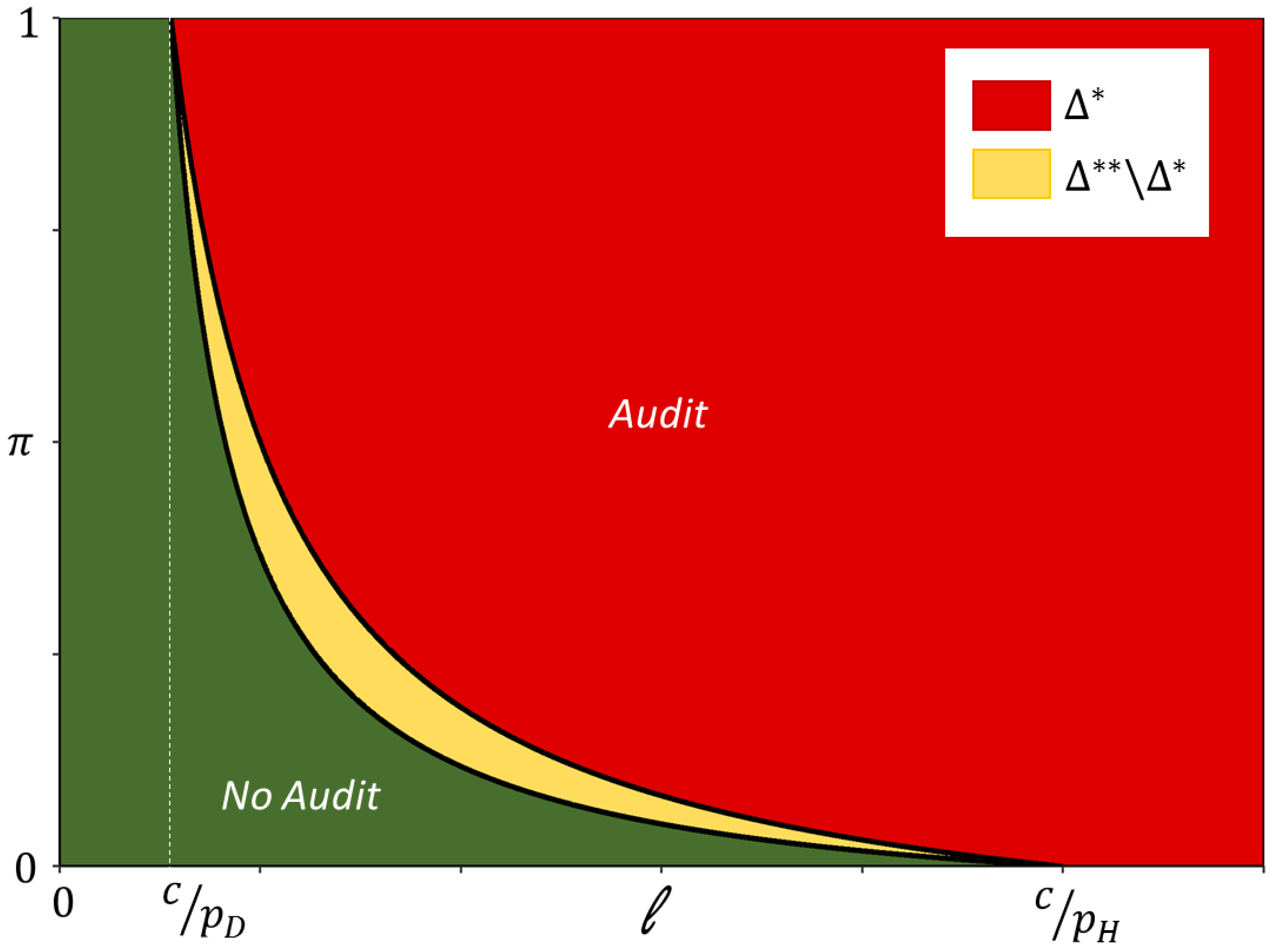
with ${\Delta }^{*}\subset {\Delta }^{**}$. These sets are illustrated in Figure 8.

4.2. Random Homogeneous Value

Let us move on now to the more interesting case where the size of the claims is a random variable drawn from a known distribution at the beginning of each period. Let ${\tilde{\ell }}_i$ denote this random variable with density $g_i(·)$ and c.d.f. $G_i(·)$ on $[0,L_i]$ for $i=0,1$. For simplicity, we assume that ${\tilde{\ell }}_i$ has the same probability distribution for both types of SPs, and thus ${\tilde{\ell }}_i$ and ${\pi }_0$ are independently distributed. The value of a claim is observed at each period before deciding to audit or not. Now, an audit strategy is written as $x_i({\pi }_i,{\ell }_i)$ at period $i=0,1$.

Lemma 4.

The inter-temporal objective function can be written as

$$\begin{array}{c}{\Omega }_0(x_0(·,·))+\gamma {\mathbb{E}}_0\left[{\Omega }_1^{*}(x_0(·,·))\right]\hfill \\ ={\int }_{[0,1]}{\int }_{[0,L_0]}\left[C({\pi }_0)+K({\pi }_0,{\ell }_0)x_0({\pi }_0,{\ell }_0)\right]g_0({\ell }_0)f_0({\pi }_0)d{\ell }_{0}d{\pi }_0,\hfill \end{array}$$

(3)

where

$$\begin{array}{cc}K({\pi }_0,{\ell }_0)\hfill & =\overline{p}({\pi }_0){\ell }_0-c+\gamma H({\pi }_0),\hfill \\ H({\pi }_0)\hfill & =\overline{p}({\pi }_0)\Phi (A({\pi }_0))+(1-\overline{p}({\pi }_0))\Phi (B({\pi }_0))-\Phi ({\pi }_0),\hfill \\ C({\pi }_0)\hfill & =\gamma \Phi ({\pi }_0),\hfill \end{array}$$

with $H({\pi }_0)>0$ if ${\pi }_0\in (0,1)$ and $H(0)=H(1)=0$, and

$$\Phi (\pi )={\int }_{{\ell }^{*}(\pi )}^{L_1}\left[\overline{p}(\pi ){\ell }_1-c\right]g_1({\ell }_1)d{\ell }_1,$$

where ${\ell }^{*}(\pi )=\frac{c}{\overline{p}(\pi )}$.

Lemmas 3 and 4 are similar and can be interpreted the same way. In particular, the two terms in the integral of Equation (3) correspond to the parts of cumulated expected proceeds according to whether they are affected by period 0 audit or not.

Proposition 3.

The optimal period 0 auditing strategy $x_0^{*}({\pi }_0,{\ell }_0)$ is such that

$$\begin{array}{c}\hfill x_0^{*}({\pi }_0,l_0)=1\mathit{if}{\pi }_0>{\pi }^{**}({\ell }_0),\end{array}$$

where ${\pi }^{**}(·):[0,L_0]⟶[0,1]$, with ${\pi }^{**}({\ell }_0)<{\pi }^{*}({\ell }_0)$ for all ${\ell }_0\in [0,L_0]$.9

Proposition 3 extends Proposition 2 to the case of claims with variable size, and its interpretation is similar. In an instantaneous setting, where learning effects would be ignored, an audit should be performed if the belief ${\pi }_0$ is larger than ${\pi }^{*}({\pi }_0)$. The threshold is decreasing with ${\ell }_0$ because the larger the claim, the larger the potential gain from auditing. When learning effects are taken into account, the threshold decreases. Claim $({\pi }_0,{\ell }_0)$ should be audited at period 0 when ${\pi }^{**}({\ell }_0)<{\pi }_0<{\pi }^{*}({\ell }_0),$ although such audit is not profitable in expected terms.

5. Conclusions

This article aimed at characterizing the learning dimension of auditing when there is a repeated interaction between auditor and auditee. The insurance claim fraud problem with potentially dishonest service providers was an application example, but the same question arises in many other settings, such as tax audits and, more generally, the verification of compliance with law. In our model, the insurer has imperfect information about the service providers’ type, and, as in the machine learning multi-armed bandit approach, he extends his audit activity beyond the desire for immediate short-term gain. Compared to a myopic strategy only focusing on short term profit, the longsighted insurer faces an inter-temporal trade-off between the immediate gain from fraud detection, and the future profit made possible by more intense auditing. This learning effect leads the longsighted insurer to increase his monitoring efforts and to put some individually unprofitable claims under scrutiny. This result remains valid when the setting is extended to a more general framework with claims of varying size: the learning effect shifts the frontier in the belief-claim size space, beyond which an audit should be performed.

These results may be extended in many directions that would be worth exploring. Firstly, we have limited ourselves to a simple two-period model. Extending our analysis to an arbitrary number of periods would allow us to take into account the possibility to exclude and replace service providers when their dishonesty becomes very probable, and also to analyze the convergence features of our model when the number of periods is large. A parallel could also be drawn between our problem and the so-called greedy/$\epsilon$-greedy strategies in bandit problems, when the latter outperform the former in the long-run (see Chapter 2 in Sutton and Barto (1998)). Another interesting issue would consist in considering the case where service providers are concerned by multiple claims at each period. The auditing strategy would have to specify how many claims will be monitored. Audit costs may also reflect a potential source of heterogeneity between claims that could lead the insurer to abstain from auditing some claims with high audit costs. Furthermore, strategic defrauders could resort to manipulation of auditing costs as a protective device against auditing (see Picard (2000)). Most importantly, our model postulates an exogenous fraud rate reflected in the frequency of invalid claims for honest and dishonest service providers. Endogenizing the frequency of invalid claims would be of particular interest, in order to study the strategic interaction between insurers, service providers and claimants, in a setting where learning and deterrence effects would coexist. Finally, the paper highlights the relevance of more intense investigations during the first stages of repeated interactions between principal and agent, and this conclusion is far more general than the insurance fraud problem. Analyzing whether this conclusion fits with actual monitoring processes is an empirical extension that would be worth exploring, for better understanding the behavior of insurers facing claim fraud and in other contexts.

References

- Bergemann, Dirk, and Juuso Valimaki. 2006. Bandit Problems. Cowles Foundation Discussion Paper No. 1551. Available online: https://ssrn.com/abstract=877173 (accessed on 27 February 2018).
- Bourgeon, Jean-Marc, Pierre Picard, and Jerome Pouyet. 2008. Providers’ Affiliation, Insurance and Collusion. Journal of Banking & Finance 32: 170–86. [Google Scholar]
- Crocker, Keith J., and John Morgan. 1997. Is honesty the best policy? Curtailing insurance fraud through optimal incentive contracts. Journal of Political Economy 106: 355–75. [Google Scholar] [CrossRef]
- Dionne, Georges, Florence Giuliano, and Pierre Picard. 2008. Optimal Auditing with Scoring: Theory and Application to Insurance Fraud. Management Science 55: 58–70. [Google Scholar] [CrossRef] [Green Version]
- Gale, Douglas, and Martin Hellwig. 1985. Incentive-Compatible Debt Contracts: The One-Period Problem. Review of Economic Studies 52: 647–63. [Google Scholar] [CrossRef]
- Mookherjee, Dilip, and Ivan Png. 1989. Optimal Auditing, Insurance, and Redistribution. The Quarterly Journal of Economics 104: 399–415. [Google Scholar] [CrossRef]
- Picard, Pierre. 2000. On the Design of Optimal Insurance Policies Under Manipulation of Audit Cost. International Economic Review 41: 1049–71. [Google Scholar] [CrossRef]
- Picard, Pierre. 2013. Economic Analysis of Insurance Fraud. In Handbook of Insurance. Edited by G. Dionne. Dordrecht: Springer, pp. 349–95. [Google Scholar]
- Sutton, Richard S., and Andrew G. Barto. 1998. Reinforcement Learning: An Introduction. Cambridge: MIT Press. [Google Scholar]
- Townsend, Robert. 1979. Optimal Contracts and Competitive Markets with Costly State Verification. Journal of Economic Theory 21: 265–93. [Google Scholar] [CrossRef]