Modeling High Frequency Data with Long Memory and Structural Change: A-HYEGARCH Model


1
Department of Actuarial Studies and Business Analytics, Macquarie University, North Ryde 2109, Australia
2
Research School of Finance, Actuarial Studies and Statistics, The Australian National University, Acton 2601, Australia
*
Author to whom correspondence should be addressed.
Risks 2018, 6(2), 26; https://doi.org/10.3390/risks6020026
Submission received: 28 February 2018
/
Revised: 20 March 2018
/
Accepted: 24 March 2018
/
Published: 26 March 2018
Abstract
:In this paper, we propose an Adaptive Hyperbolic EGARCH (A-HYEGARCH) model to estimate the long memory of high frequency time series with potential structural breaks. Based on the original HYGARCH model, we use the logarithm transformation to ensure the positivity of conditional variance. The structural change is further allowed via a flexible time-dependent intercept in the conditional variance equation. To demonstrate its effectiveness, we perform a range of Monte Carlo studies considering various data generating processes with and without structural changes. Empirical testing of the A-HYEGARCH model is also conducted using high frequency returns of S&P 500, FTSE 100, ASX 200 and Nikkei 225. Our simulation and empirical evidence demonstrate that the proposed A-HYEGARCH model outperforms various competing specifications and can effectively control for structural breaks. Therefore, our model may provide more reliable estimates of long memory and could be a widely useful tool for modelling financial volatility in other contexts.
1. Introduction
One important research topic in statistics and econometrics is analyzing economic and financial time series, in particular, investigating the dynamic behavior of macroeconomic and financial variables. Traditional models adopt a convenient assumption of constant conditional variance, which ignores fluctuations in the second-order structure of time series. Following the Autoregressive Conditional Heteroskedasticity (ARCH) process introduced by Engle (1982), models with time-varying conditional variances depending on the past realizations have become popular and been proven useful in the past decades. For example, Weiss (1984) models and discusses thirteen U.S. macroeconomic time series using the Autoregressive Moving Average (ARMA) models with ARCH errors. Extended from it, the Generalized ARCH (GARCH) process introduced by Bollerslev (1986) replaces lagged sample variances in the ARCH process with lagged conditional variances, which is analogous to the ARMA structure. Despite its popularity, the GARCH model has several non-negligible drawbacks, including the inability to capture the long memory behavior of high frequency time series.
Long-memory persistence commonly exists in the studies of the volatility of high frequency financial time series (see, for example, Bollerslev and Mikkelsen 1996; Dacorogna et al. 1993; Ding et al. 1993; Granger and Ding 1996b). A widely appreciated definition of the long memory is provided by Diebold and Inoue (2001). It states that financial time series has a long memory persistence measured by d, if , where . To capture this feature, long memory extensions of the GARCH model have been introduced by various researchers; famous examples include the Fractionally Integrated GARCH (FIGARCH) model proposed by Baillie et al. (1996) and the Hyperbolic GARCH (HYGARCH) model proposed by Davidson (2004). Compared with the GARCH model, both the FIGARCH and the HYGARCH models are capable of describing the observed long-run dependencies in the conditional variances of financial time series.
Despite the growing amount of research on the long memory feature of time series, many studies are unconvinced about its validity for the volatility processes. Particularly, it has been proved that structural changes can partly explain some extremely persistent volatility processes, and can also induce a time series to have long memory behavior. Lamoureux and Lastrapes (1990) originally showed that structural changes in the unconditional variance of stock returns may generate overestimated extremely persistent volatility. Subsequent theoretical explanations have been presented by Morana (2002) and Hillebrand (2005). Moreover, Diebold and Inoue (2001) have demonstrated that structural change is related to long memory, and both features are easily confused with each other. Therefore, a more appropriate volatility model would be able to consider long memory and structural change simultaneously. Similar opinions can be found in studies by Beine et al. (2001), Morana and Beltratti (2004), and Martens et al. (2004).
This paper proposes an Adaptive Hyperbolic Exponential GARCH (A-HYEGARCH) process. It is designed for modeling the long memory of high frequency financial time series with structural changes. This model incorporates the structure of Exponential GARCH (EGARCH) model discussed by Nelson (1991) into Davidson (2004)’s HYGARCH model, further considering a time varying deterministic component in the flexible functional form provided by Gallant (1984). Those features enable the A-HYEGARCH model to nest stochastic long memory and deterministic break processes. As an improvement over the original HYGARCH specification, the proposed model requires many fewer and much simpler parameter constraints to ensure the non-negativity of the conditional variance. Therefore, the estimation process is expected to be more efficient and accurate. Compared with related approaches to model the structural change, the employed adaptive function does not require any further information of the number or locations of change points (Baillie and Morana 2009).
To demonstrate the usefulness of A-HYEGARCH model, we firstly conducted a series of Monte Carlo simulations. It is shown that the A-HYEGARCH can effectively mitigate the upward bias in the estimated values of the long memory parameter d in the presence of structural breaks. Apart from that, we investigate its practical performance using empirical studies on four world stock indexes. More specifically, our data range from 1 January 2008 to 31 December 2011 for each of four popular world-wide stock exchange indexes, including: (1) the Standard & Poor’s 500 (S&P) index, which consists of 500 large companies having stock listed on the New York Stock Exchange and NASDAQ; (2) the Financial Times Stock Exchange 100 (FTSE), which consists of 100 companies listed on the London Stock Exchange; (3) the S&P/ASX 200 (ASX) index, which consists of 200 companies listed on the Australian Securities Exchange; and (4) the Nikkei 225 (Nikkei) index, which consists of 225 Japanese companies listed on the Tokyo Stock Exchange. With the existence of 2008 Global Financial Crisis (GFC), the estimated long-memory parameter of A-HYEGARCH is consistently smaller and more reliable than the long-memory GARCH models that do not allow structural change. On the other hand, when compared with three other adaptive GARCH-type models (A-FIGARCH, A-FIEGARCH and A-HYGARCH), the A-HYEGARCH model still demonstrates outstanding performance. For instance, it consistently outperforms the competing models according to both Akaike information criterion (AIC) and Bayesian information criterion (BIC). Thus, our A-HYEGARCH framework could be a widely useful tool for modelling financial volatility in other contexts including the financial risk management.
The reminder of this paper proceeds as follows. Section 2 reviews two popular long memory GARCH-type models, together with their advantages and constraints. Structural changes observed in financial volatility and the related adaptive models are discussed in Section 3. Section 4 explains the A-HYEGARCH model proposed in this paper, and presents evidence of the model’s effectiveness to estimate long memory parameter in the presence of structural changes via Monte Carlo studies. Section 5 describes the empirical applications and Section 6 concludes the paper.
2. Long Memory GARCH-Type Models
2.1. FIGARCH Model
To model the long-term persistence, Engle and Bollerslev (1986) developed the Integrated GARCH (IGARCH) model as an extension to the original GARCH model. It is argued that IGARCH models have a property called “persistent variance” since any shocks to the conditional variance, either happened today or in the past, will persist indefinitely into the future. However, Nelson (1990) showed that the IGARCH process without drift would definitely converge to zero with probability one, in finite steps. Hence, IGARCH models are generally considered as short memory models by researchers (Davidson 2004; Granger and Ding 1996a). Additionally, the IGARCH process is neither covariance stationary nor does it have well-defined unconditional variance, although it is possible to be strictly stationary and ergodic (Nelson 1990).
Baillie et al. (1996) generalized the IGARCH model to a new class named Fractionally Integrated GARCH (FIGARCH) models, with the purpose of explicitly describing the long memory behavior of the conditional variances of financial time series. Following the formulations of ARCH and GARCH models, for a discrete times real-valued stochastic process , Baillie et al. (1996) parameterized the FIGARCH ( model as:
where is the conditional variance of , . In particular, is an identically and independently distributed (iid) innovation sequence following a known distribution with zero mean and unit variance.1 The lag polynomials are defined as and . If all roots of and lie outside the unit circle, the FIGARCH model can be rearranged into an ARCH( representation as
with and .
To ensure that the FIGARCH ( process described in Equation (1) is well-defined, and the conditional variance remains positive for all t, generally, all the parameters in Equation (2) must be non-negative. In other words, 0, and for all k. More detailed conditions for the non-negativity of in Equation (2) are given by Conrad and Haag (2006) who extended the results of Nelson and Cao (1992) to the FIGARCH ( framework and derived necessary and sufficient conditions for and sufficient conditions for .
As a direct extension to IGARCH, the FIGARCH model has its short-run dynamics described by the conventional GARCH parameters (s and s). In contrast to the GARCH model where shocks to the conditional variance dissipate quickly at an exponential rate, shocks of FIGARCH exhibit hyperbolic decays. This feature of the FIGARCH model stems from the fractional differencing factor . According to Granger and Joyeux (1980) and Hosking (1981), the fractional differencing factor has an expanded form as , with
Equation (3) indicates that decays hyperbolically rather than geometrically, implying impulse responses to shocks in the conditional variance of FIGARCH models die out slower than those of GARCH models.
Although the FIGARCH process is designed to model the long memory behavior of financial time series, some researchers are sceptical about it. For example, Davidson (2004) argued that the FIGARCH model’s long memory property is misleading: firstly, when d approaches boundaries of its defied interval (0, 1), the FIGARCH model will behave quite close to either the GARCH model or the IGARCH model. Therefore, the FIGARCH model acts as a role of intermediate model between the stable short memory GARCH and IGARCH models, but with longer memory than either one. The memory of the FIGARCH model will suddenly jump to the negative infinity if d is close enough to its boundaries. Secondly, 1 always holds regardless of the value of d, implying that the FIGARCH model belongs to the “knife-edge-nonstationary” class of models, which nests the IGARCH (1). Hence, just like IGARCH, the FIGARCH model does not have well-defined unconditional variance and is not covariance stationary. Such limitations of the FIGARCH model motivate researchers to develop other long memory volatility models for financial time series.
2.2. HYGARCH Model
To overcome the issues of FIGARCH, Davidson (2004) proposed the HYGARCH model, which also has hyperbolically decaying impulse response coefficients. The HYGARCH( model is defined as:
where , ; , and are defined as before. The HYGARCH model reduces to the GARCH model when or and reduces to the FIGARCH model when If d happens to take the value of 1, then the HYGARCH model will become either a stationary GARCH , an IGARCH or a GARCH with explosive conditional variances.
If all roots of and lie outside the unit circle, the HYGARCH model can be rearranged into an ARCH( representation as
with , where . This expression implies that ARCH( coefficients of the HYGARCH model are constructed as a weighted average of the ARCH( coefficients from the GARCH and the FIGARCH model, with weights and , respectively. Hence, the conditional variance equation of the HYGARCH model can be rewritten as
It can be seen from Equation (6) that the conditional variance equation of the HYGARCH model has a short-run GARCH component and a long-run FIGARCH component. In general, the HYGARCH model will be covariance stationary for any and .
Similar to GARCH and FIGARCH models, there are conditions for HYGARCH models to ensure conditional variances remain positive for all t. Conrad (2010) explored this topic in detail and gave specific necessary and sufficient conditions for the non-negativity of the conditional variance of the HYGARCH( model. However, although not technically restrictive as the conditions for GARCH and FIGARCH, those conditions for HYGARCH are even more complicated and can be very possibly violated in application.
Another important limitation of the HYGARCH model (and other long-memory GARCH models) exists when structural breaks occur in data. Among existing studies, Lamoureux and Lastrapes (1990) attempted to adjust for change of regimes in the conditional variance intercept of the GARCH model fitted to 30 randomly picked CRSP stocks. Substantially lower estimates of the long memory parameter d are observed. Choi et al. (2010) compared estimates of d in HYGARCH models before and after adjusting for structure breaks. They found that, when structure breaks are present, d tends to be overestimated. Similar results can also be found in recent studies like Günay (2014).
3. Structural Change and Relevant Models
3.1. Structural Change in Time Series
In relation to the cause of structural change, empirical research has shown that structural change in financial time series often associates with permanent changes in the fundamental structure of an economy (Balke and Fomby 1991), financial crises (Cerra and Saxena 2005; Jeanne and Masson 2000) or even government abrupt changes of monetary and/or fiscal policies (Hamilton 1988; Sims and Zha 2006). Figure 1 displays the movements of the ASX stock index over the period 1 January 2008 to 31 December 2011, during which time the major financial markets in the world are experiencing recessions. Two completely different volatility structures of returns can be clearly observed in the figure. The red dashed line indicates the structural change point detected by the Mood test using the Nonparametric Change Point Model (NPCPM), which are described in Section 4. An obvious change in its return volatility is observed in early 2009. Such structural changes are likely widespread in financial and economic time series, and relevant persuasive empirical evidence can be found in Stock and Watson (1996).
As described above, structural change is related to long memory and can lead to overestimated d. Thus, due to the existence of structural change in practice, the application of the original FIGARCH and HYGARCH is limited in practice. An extension of those models to control for the effect of structural breaks is therefore of particular interest to provide more reliable estimates of long memory.
To model the structural change within the GARCH framework, various approaches have been studied in the literature. Hamilton and Susmel (1994) noticed the possible influence of extreme shocks to the fundamental structure of economy and incorporated the regime-switching model with ARCH volatility forecasting methodology. Gray (1996) combined the generalized regime-switching (GRS) model and the GARCH process in modeling interest rates, assuming state-dependent Markov transition probabilities and GARCH parameters. This model demonstrates considerably lower estimates of persistence in conditional variance and better out-of-sample forecasting results, compared to simple single-regime models. However, there is little research studying the incorporation of the regime switching feature into the long memory GARCH model. More importantly, such a model would require a reliable estimate of the number of volatility states, which is still an unresolved technical issue. In addition, with the increase of this number, the total number of parameters to be estimated for a regime-switching model can rise exponentially. This could become unmanageable and lead to computational inefficiency in practice. More discussions regarding this can be found in Shi and Ho (2016).
3.2. Adaptive-FIGARCH Model
To address the issue of regime-switching approach, existing studies have incorporated the structural breaks into long memory models using effective alternative parametric features. Baillie and Morana (2009) introduced the Adaptive-FIGARCH (A-FIGARCH) model, which is designed to account for both long memory and structural change in financial time series.2 The A-FIGARCH model consists with two components—a stochastic long memory part and a deterministic break process element. Following Baillie et al. (1996), the A-FIGARCH(p, d, q, k) model can be expressed as:
where . The main difference between the A-FIGARCH model and the conventional FIGARCH model is the inclusion of the time varying intercept . The A-FIGARCH model can be reduced to the standard FIGARCH model by setting .
The intercept in the A-FIGARCH model follows the Fourier flexible functional form originally proposed by Gallant (1984), which has been adopted in influential finance research like Andersen and Bollerslev (1997, 1998). According to Baillie and Morana (2009), this flexible functional form is able to accurately approximate abrupt structural changes, such as discontinuous shifts3. Hence, with a time varying , modelling structural change is attainable by selecting the proper frequency (i.e., the value of k) for the intercept term. Unlike the regime-switching approach, A-FIGARCH model with a larger k always nests that with a lower k. Thus, a general likelihood-ratio test can be adopted to test the number of k. In addition, Baillie and Morana (2009) suggests a parsimonious number like 2 or 3 is usually sufficient, although a larger number may be required by data with a longer sample period. In any case, without a filtering approach to commutate the likelihood of regime switching GARCH models (see Shi and Ho (2016) for details), the computational burden of the Adaptive-type GARCH model is much lower. The number of total parameters also increases slowly with the growth of k.
Non-negativity conditions for the conditional variance of A-FIGARCH model inherit those of the standard FIGARCH model. The initial sufficient condition given by Baillie et al. (1996) in the FIGARCH paper requires that , and . According to Conrad and Haag (2006), the restriction on could be released, with the less restrictive necessary and sufficient conditions involving only parameters and . Therefore, it is safe to include the trigonometric terms in , with no need to worry about violating nonnegative conditions for the conditional variance of A-FIGARCH models.
As described above, neglecting structural breaks leads to overestimated long memory measure. Simulation results provided by Baillie and Morana (2009) show that the estimate of long memory parameter d obtained from the A-FIGARCH model generally has smaller bias and lower root mean square error than the standard FIGARCH model. This demonstrates that inclusion of the trigonometric components in the intercept can effectively mitigate the upward bias in the estimate of long memory parameter d from the standard FIGARCH estimation. A direct interpretation of this suggests that the Fourier flexible functional form of the A-FIGARCH model performs well in modeling the structural change in the conditional variance. Baillie and Morana (2009) also point out that, when the degree of persistence is higher (e.g., ), the reduction of estimated d using A-FIGARCH over that with FIGARCH is higher.
Despite its effectiveness in estimating d, A-FIGARCH model still has issues as those of FIGARCH. It also does not have well-defined unconditional variance and is neither strictly stationary nor ergodic. Furthermore, the accuracy of long memory measure is questionable, like described in Section 2.2. A natural extension is to apply the adaptive form to the better parametrised HYGARCH specification. However, the complex non-negativity constraints would still apply for the potential A-HYGARCH model. This may cause problems in practice, due to the bounded optimization procedure (i.e., numerical maximization of the log-likelihood function over selected intervals) employed in the estimation of model parameters. This may potentially lead to computational inefficiency and even numerical inaccuracy, especially when true values of parameters are close to the boundaries of constraints.
4. The A-HYEGARCH Model
Nelson (1991) introduced the Exponential GARCH (EGARCH) model that successfully releases the non-negativity constraints of the original GARCH model. Moreover, as noted by early study of Black (1989), volatility of stock returns tend to increase in response to a drop in the stock price, possibly caused by the accumulating financial and operating leverage in this situation. By squaring the lagged residuals, the original GARCH model loses information contained in the sign of past residuals, resulting in conditional variance responding symmetrically to positive and negative residuals. In contrast, the EGARCH model contains an important precedent of incorporating asymmetric terms into the conditional variance equation. An extension of EGARCH to allow long memory leads to Bollerslev and Mikkelsen (1996)’s FIEGARCH model. A HYEGARCH specification could then be further derived.
4.1. Step 1: HYEGARCH Model
As described in Section 2, the HYGARCH model is capable of dealing with highly persistent volatility processes. The GARCH and FIGARCH components found in HYGARCH models together add great flexibility to modeling persistent volatility processes, as they dominate in either the short- and long-run, respectively. Following this idea, a HYEGARCH model can be proposed by nesting a short-memory model (the EGARCH model) and a long-memory model (the FIEGARCH). Such a model would have hyperbolically decaying memory and with a EGARCH-type conditional variance equation.
More specifically, a HYEGARCH( process can be defined as
where and with . The lag polynomials follow those in the HYGARCH specification, i.e., and . Clearly, when , HYEGARCH reduces to the EGARCH model, whereas results in the FIEGARCH model.
Following the Maclaurin expansion of , upon replacing d by , the fractional differencing factor has the same binomial expansion as in Equation (3). That is,
where This demonstrates that shocks to the conditional variances of HYEGARCH model decay hyperbolically.
The conditional variance equation of HYEGARCH model can be rewritten to a more general form as follows:
where and are real non-stochastic sequences provided that the process is well defined. Note that does not necessarily have a variance of 1, and it can be any white noise process with definite variance. The function can be any measurable function, while here it is assumed to be the same form as in the FIEGARCH (EGARCH) model with the purpose of allowing for asymmetric response to positive and negative shocks.
4.2. Step 2: A-HYEGARCH Model
In analogy to Baillie and Morana (2009)’s generalization of the FIGARCH model to the adaptive framework, we propose that the HYEGARCH model introduced above can also be extended to an A-HYEGARCH model. Therefore, it would also allow for structural change in modelling time series. More specifically, an A-HYEGARCH model is defined as
where is defined as in the A-FIGARCH model, and all other variables are defined as in the HYEGARCH model.
For a general FIEGARCH process, Lopes and Prass (2014) have shown that, when has finite mean, and and are not both equal to zero, is a strictly stationary and ergodic process. If , then is a white noise process with the following variance specification
Nelson (1991) pointed out that the stationarity and ergodicity criterion is exactly the same as for any general linear process with finite variance innovations. Hence, we directly extend their theorem to our A-HYEGARCH mode. Nelson (1991) also stated that, in many applications, an ARMA process gives a parsimonious parameterization for .
For the A-HYEGARCH defined in Equation (11), let be the polynomial with the following form
Then, for all the coefficients satisfy as k goes to infinity. Hence, it can be shown that the coefficients in Equation (10) converge to a finite order of k, as k goes to infinity. This property is important as the asymptotic representation is essential for establishing the necessary condition for square summability of and for the criterion of Theorem 2.1 in Nelson (1991). Furthermore, one can conclude that this theorem holds for the A-HYEGARCH model if and only if , and at the same time . In addition, as noticed above, shocks to the logarithm of conditional variance also decay slowly at a hyperbolic rate, which allows for the long-run dependency.
Using those results, we notice that, for an A-HYEGARCH(p, d, q, k) process, is stationary (strictly and weakly) and ergodic when . The holds almost surely. Moreover, and are both strictly stationary and ergodic processes. Therefore, would be a white noise process, and becomes an ARFIMA process (Lopes and Prass 2014). Therefore, we can conclude the following properties:
Property 1
When the autocorrelation function of is
Property 2
If and , the process is invertible.
Finally, although in the GARCH family model is all originally assumed to be Gaussian, the Student’s t distribution is more appropriate in practice to model the fat=tail property. For example, Bollerslev (1987) advocated the benefit of using the Student’s t distribution in his study of exchange rates and stock indexes. Davidson (2004) also adopted the Student’s t distribution in the analysis of various exchange rates using his HYGARCH models. Thus, in the rest of this paper, we assume that follows a Student’s t distribution rather than the Gaussian.
4.3. Estimation of A-HYEGARCH Models
In this section, we report Monte Carlo simulation evidence on the estimation of A-HYEGARCH models for different data generating processes (DGPs) of HYEGARCH with structural change. All models in this section assume that follows the Student’s t distribution with 3 degrees of freedom. We specify an uncorrelated process for the mean in all the experiments, with conditional variance processes exhibiting various forms of long memory behaviors with and without structural breaks. As A-HYEGARCH (HYEGARCH) models contain weighted fractional differencing factor which is also found in standard HYGARCH models, the set of parameters in this study are chosen to be close to those in Conrad (2010)’s simulation study of the HYGARCH model. In addition, following Baillie and Morana (2009)’s simulation study design, we choose the values of d and limit that (0,0), (1,0) or (1,1). More specifically, we consider , , , , and the long memory parameter . Note that corresponds to moderate persistence in volatility process while is very close to the non-stationary region (, indicating high persistence in . In addition, the structural change is assumed for only, the values of which are discussed below.
To generate samples from HYEGARCH DGPs with structural change, we follow 3 steps below. Notice that Step 3 acts as the core part of this simulation study, and it must be repeated for each model and each replication. Step 1 is also repeated for reach replication, while Step 2 only needs to be performed once for each model. Following Baillie and Morana (2009), we consider 500 Monte Carlo replications with 10,000 observations simulated for each. The first 9000, 8000 and 7000 are then discarded to avoid simulation errors, resulting in sample sizes , respectively.
Step1: Set , and get an sample , where m represents the number of extra burn-in data generated.
Step 2: Choose appropriate designs for the intercept term in each model. In this research, we consider three different designs:
Design 1 () assumes a constant intercept , and corresponds to the standard experiment setting where no structural breaks are allowed in the conditional variance.
Design 2 () adopts the permanent break structure which is used by Baillie and Morana (2009) in their research and has one step change in the intercept right at the middle of the sample. At the break point, the intercept jumps from 0.1 to 0.5 without bouncing back in the future. Hence,
Design 3 () has two step changes occurring at one-third and two-thirds of the way throughout the sample, with the intercept jumping from 0.1 to 0.5 at the first break point and bouncing back to 0.3 at the second break point. Hence,
Step 3: The sample is obtained using the specification described in Equation (10) () with chosen values of parameters and extra burn-in data deleted to avoid start-up problems.
In terms of the estimation, as discussed above, we assume that the innovation sequence follows the Student’s t distribution with degrees of freedom. The log-likelihood function applied to all models of this paper can then be described as follows:
where the vector of unknown parameters is denoted by
We maximize Equation (15) with the help of statistical packages in R (R Core Team 2017) to obtain estimate of , denoted by .
Maronna (1976) has proved the existence, uniqueness, consistency, and asymptotic normality of Student’s t long-likelihood estimators. For instance, under general assumptions, if there exists such that, holds for every hyperplane H, then the equations obtained by differencing Equation (15) have a unique and consistent solution.4
To assess the performance of maximum likelihood estimator , we calculate the Monte Carlo bias (Bias), the root mean square error (RMSE) and the standard error (SE) of the estimated long memory parameter d. For any model considered, let denote the estimated value of d in the n-th replication, where . Then, the performance measures are defined as
Table 1 summarizes estimation results of the A-HYEGARCH models with (equivalent to ordinary HYEGARCH models) for the HYEGARCH DGP with design 1 (no structural change). We noticed that the obtained estimates of the long memory parameter d have very small bias when the sample size T is large. This result is consistent for the three values assumed for d and across all three selections of T. For instance, the estimation is generally smaller than 5% when the sample has over 3000 simulated data. The HYEGARCH DGPs with has the most significant reduction in estimation bias, from 0.0264 reduced to 0.0015 when sample size increases from 1000 to 5000.
Table 2 reports estimation results for A-HYEGARCH models with . As revealed in the table, increasing the value of k will not significantly change estimation bias of the long memory parameter d. Generally speaking, the bias of the estimated d is less than 5%, which indicates great accuracy of A-HYEGARCH models in the absence of structural change. Table 2 also reports significant reductions in standard errors of estimates of long memory parameter d as sample sizes increase. Using A-HYEGARCH models as an example, when , a five-fold increase in sample size results in the SE dropping by 27%; when , a five-fold increase in sample size results in the SE dropping by more than 40%. This is consistent with the ordinary asymptotic property.
There is another important result obtained by comparing Table 1 and Table 2. More than half model designs show reduction in RMSE after adopting adaptive structure. As d increases, however, the reduction in the degree of RMSE tend to decrease. These results suggest that the A-HYEGARCH model has the same property as A-FIGARCH regarding the use of the adaptive structure. No additional cost will be incurred by adopting the time dependent intercepts, regardless of the chosen number of k in the conditional variance equation. According to Baillie and Morana (2009), this result suggests that the intercept used, which follows Gallant (1984)’s flexible functional form with more than one pair of trigonometric components, can adjust for some uncertainties in the estimation of the long memory parameter d.
Table 3, Table 4 and Table 5 provide simulation results for various A-HYEGARCH models for HYEGARCH DGPs subject to structural change designs. From Table 3, it can be seen that most A-HYEGARCH(0,d,0,k) models appear to have smaller estimation bias for the structural change design than the design. With an intercept term containing three pairs of trigonometric components (), the A-HYEGARCH model reports estimation biases of (when for the design and () for the design, both are the smallest results for the corresponding DGP designs. It appears that the value of k at which the estimation bias of the long memory parameter d reaches its minimum is related to the underlying number of structural changes. Based on our simulation results, the optimal value of k for A-HYEGARCH models is very likely to be equal to the number of regimes of the data plus one. More importantly, most of the A-HYEGARCH () models produce smaller biases compared to the HYEGARCH ().
Table 4 reports simulation results for estimates of A-HYGARCH models. For the design, the smallest estimation bias produced by A-HYEGARCH models equals to 0.0090, which is achieved at . The smallest estimation bias for the design produced by the same class of models equals to 0.0999, which is achieved at . This is consistent with our observation above. In addition, A-HYEGARCH still outperforms HYEGARCH in producing a more accurate estimate of d.
Table 5 presents simulation results for estimates of A-HYGARCH models. Apart from the designs with , simulation results here have generally consistent features with those shown in Table 3 and Table 4. Note that a constraint of was imposed in the maximum likelihood estimation to ensure stationarity. When the true value of d is approaching 0.5 (the case ) , this may lead to some negative bias observed for A-HYEGARCH models.
In the analysis above, we focus with the DGPS with . As sample size increases, the estimation bias and standard error both tend to decrease. The consistent reduction of Bias and SE, and hence RMSE, accompanying the growth of sample size provides a possibility for further reducing the estimated root mean square errors. With more replications and larger sample sizes, we anticipate greater stability in the simulation results.
In general, the A-HYEGARCH model consistently outperforms HYEGARCH across different simulation designs with and without structural change. Thus, inclusion of the trigonometric components in the A-HYEGARCH model appears to effectively mitigate the upward bias in estimating d. This suggests the usefulness of A-HYEGARCH to model financial sequence in practice. Our empirical evidence to demonstrate this is discussed in the next session.
5. Empirical Results
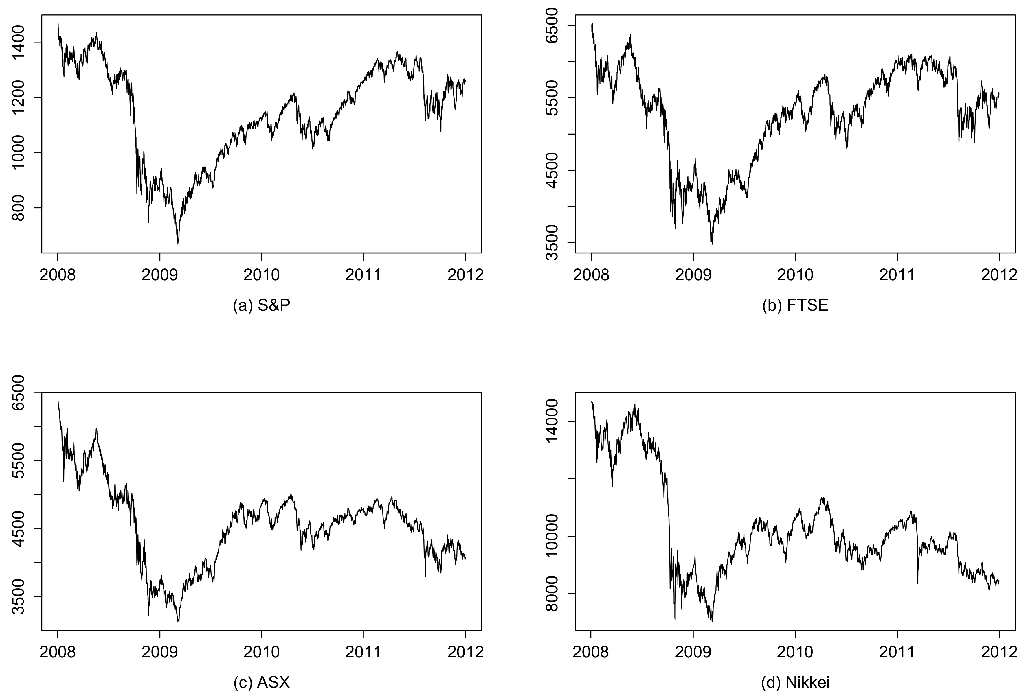
We apply various (adaptive) long-memory GARCH-type models studied in this paper to four world stock indexes, comparing their performances at modeling return volatility. They are: (1) the Standard & Poor’s 500 (S&P) index, which consists of 500 large companies having stock listed on the New York Stock Exchange and NASDAQ; (2) the Financial Times Stock Exchange 100 (FTSE), which consists of 100 companies listed on the London Stock Exchange; (3) the S&P/ASX 200 (ASX) index, which consists of 200 companies listed on the Australian Securities Exchange; and (4) the Nikkei 225 (Nikkei) index, which consists of 225 Japanese companies listed on the Tokyo Stock Exchange. Our dataset is composed of hourly closing prices for the four indexes over the period 1 January 2008 to 31 December 2011. The four time series are plotted in Figure 2.
For each index, the return in the percentage series is defined as the logarithm of the hourly closing price differences times 100, that is, , where is the hourly closing price recorded in the corresponding national currency at time t. Figure 3 presents plots of the return series and the absolute return series (as proxy for conditional volatility) for each index. Many stylized facts of financial time series such as stationarity with an approximate zero mean and clusters of volatility can be identified in the figure. The autocorrelation of the original and absolute return series is shown in Figure 4, which presents more stylized facts such as the absence of autocorrelations in the mean level and the slow decay of autocorrelation in the volatility. Such slow decays suggest large persistence in the volatility processes for the stock index returns. Hence, long memory models are expected to provide better performance in modeling the conditional variance of the chosen financial series.
Table 6 displays a group of summary statistics for the stock index returns. It can be seen that, though there are some large deviations, the mean value is very close to 0 for all indexes. FTSE and ASX have standard deviations smaller than 0.25, while S&P and Nikkei have slightly larger variations. S&P is positively skewed in contrast to the other three indexes, which are all negatively skewed. All indexes have kurtoses significantly larger than 0, suggesting that none of them has a Gaussian distribution. Normality tests results reported include p-values from the Kolmogorov–Smirnov and Jarque–Bera tests. All p-values are quite close to 0, indicating the rejection of the null hypothesis that selected index returns are normally distributed. Further, we present the Ljung–Box test results, which indicate that significant autocorrelations exist in all absolute return series, which confirms with findings drawn from Figure 4 indicating significant ARCH effects for all indexes. Finally, most index pairs exhibit weak positive correlations during our sample period. The correlation between Nikkei and FTSE, and that between Nikkei and S&P, however, are weakly negative.
5.1. Procedure of the A-HYEGARCH Model Fitting Empirical Data
Before fitting the empirical data, we summarize the procedure of our A-HYEGARCH model as a flowchart demonstrated in Figure 5. First, high-frequency data are tested for the existence of structural breaks. If they are not present, an ordinary HYEGARCH () can be fitted. Otherwise, we need to determine the value of k. As discussed above, Baillie and Morana (2009) suggest that a parsimonious choice like 1 or 2 is normally a good start. Structured tests can also be performed (such as the likelihood-ratio test) to obtain an optimal choice. Popular criteria like AIC and/or BIC may also be considered. Finally, if the empirical data are fat-tailed/leptokurtic, an appropriate choice of fat-tailed distribution like Student’s t, rather than the Gaussian, will be assumed for the innovation sequence. The parameters are therefore estimated by maximizing the corresponding (log-)likelihood function.
5.2. Structural Change Test
To demonstrate the potential usefulness of the adaptive long-memory GARCH-type models, we firstly conduct formal structural change tests to confirm that they significantly exist in the dataset investigated. More tests are then conducted to detect structural breaks in the log-return series of the four indexes. According to Ross (2013), this Mood-type test employed can only be applied to independent time series. Hence, we firstly standardized the return series by dividing the conditional standard deviation derived from a GARCH(1,1) model.5 Then, we apply the Nonparametric Change Point Model (NPCPM), which is proposed by Ross (2013) based on the seminal work of Mood (1954), to detect existence and locations of structural change points. Figure 6 presents the hourly return and change points for stock indexes S&P, FTSE, ASX and Nikkei over the period 1 January 2008 to 31 December 2011. The vertical red dash lines indicate the structural change points in hourly returns detected by using the Mood test and NPCPM algorithm. There are 5, 5, 1 and 1 change points discovered for S&P, FTSE, ASX and Nikkei, respectively. Hence, adaptive long-memory GARCH-type models are expected to provide more accurate results. Those without the adaptive feature are also fitted for comparison.
5.3. Model Performance Comparison
We firstly consider the four ordinary long-memory GARCH(1,d,1) models: FIGARCH, HYGARCH, FIEGARCH and HYEGARCH. Their adaptive extensions are subsequently fitted6. The estimation results are reported in Table 7 for the non-adaptive models and in Table 8 and Table 9 for the adaptive models. The effectiveness of the adaptive extension can then be observed. Apart from that, other information can be obtained by contrasting HYGARCH to FIGARCH specification, for GARCH an EGARCH frameworks, respectively. Therefore, we consider the following four pairs of model comparisons:7
From Table 7, all non-adaptive models produce considerably large estimated d, indicating significant persistence for all indexes. For instance, estimated d for the S&P index are 0.9611 by FIGARCH model and 0.8837 by HYGARCH model. These values are quite close to the upper bound of the long memory parameter in the corresponding models, suggesting extreme persistence in the conditional variance of S&P return series. This is consistent without observations in Figure 3. Notice that long memory parameters estimated by HYGARCH are considerably smaller than that produced by FIGARCH for all indexes. Since structural change is present, a lower d is expected to be more accurate. This is consistent with Davidson (2004), who argues that the inclusion of in the HYGARCH specification would improve the accuracy of long memory measure. As for Pair2, HYEGARCH and FIEGARCH tend to produce similar long-memory estimates8. Overall, all of the large estimates of d demonstrate concerns of non-stationarity.
From Table 8 and Table 9, estimated d are much smaller when the adaptive feature is allowed. This result is consistent across all four indexes, with the most remarkable reductions found in estimates for the ASX and Nikkei stock indexes. Using ASX as an example, we compare estimates of d produced from Pair3 and Pair1 models. It shows that the A-FIGARCH model can bring down estimated d from 0.8867 (produced by the FIGARCH model) to 0.7333. The reduction for the HYGARCH specification is from 0.5944 to 0.5422. These results demonstrate the effectiveness of adaptive long-memory GARCH models without logarithm transformation for the conditional variances. The reductions for the EGARCH-type pairs are more significant. In contrast to a large estimate over 0.85 when adaptive feature is not considered, A-FIEGARCH and A-HYEGARCH models result in 0.2122 and 0.3450 for the estimated d, respectively. This result further confirms that structural change has induced the ASX return series to display misleading long memory behavior, if it is not appropriately controlled for. More specifically, both FIEGARCH and HYEGARCH suggest strong persistence, non-stationarity and non-invertibility (as ), whereas their adaptive extensions argue moderate long-memory, stationarity and invertibility. Estimation results associated with the other return sequences demonstrate consistent findings, although reductions in estimates of d vary.
Finally, various model diagnostics and evaluation criteria are reported in Table 10 for model comparison among the four adaptive long-memory GARCH models. Table 10 shows that A-FIEGARCH models and A-HYEGARCH models outperform the other two as suggested by both AIC and BIC. In particular, A-HYEGARCH is the optimal model in most cases. Despite the variation among model diagnostics, there is no material difference observed for the four adaptive models in all cases.
To sum up, all of our empirical study results demonstrate the usefulness of A-HYEGARCH model in practice, including the adaptive feature to control for the detected structural change being proven substantially effective, which is shown to be evident by the reduction in estimated d. For another, the A-HYEGARCH model outperforms other competing adaptive long-memory GARCH models in terms of model evaluation results. Thus, our proposed A-HYEGARCH model can be a widely useful tool to study long memory in practical contents, for which structural change is inevitable.
6. Conclusions
This paper proposes a new A-HYEGARCH process to model high frequency financial volatility, which accounts for both long memory and structural change features. By adopting the natural logarithm of the conditional variance, no constraints are needed to ensure its non-negativity. This particular structure of the A-HYEGARCH model releases the complex restrictions that exist in many popular and related models, like the HYGARCH. Moreover, to control for the structural change, the A-HYEGARCH model employs a time-varying intercept using the flexible functional form specified by Gallant (1984). As argued by Baillie and Morana (2009), this feature does not require pre-testing the number or locations of structural change points before fitting to the data. Furthermore, the inclusion of the trigonometric components can effectively mitigate the upward bias in the estimate of the long memory parameter when structural changes occur.
A series of Monte Carlo studies are conducted to demonstrate effectiveness of the A-HYEGARCH model with and without the presence of structural changes. Compared with the ordinal HYEGARCH models, our results indicate that the A-HYEGARCH model can significantly reduce the overestimated long-memory parameter when structural changes do exist. In addition, it can perform at least as well when no structural change is assumed.
The usefulness of the A-HYEGARCH model in practice is also presented with empirical evidence. We consider four world-wide popular stock indexes: S&P 500, the FTSE 100, the S&P/ASX 200 and the Nikkei 225. Comparing with the (A-)FIGARCH, (A-)FIEGARCH, (A-)HYGARCH and HYEGARCH, the proposed A-HYEGARCH can lead to more reliable estimates of the long memory parameter and improved fitness in most cases. Hence, the A-HYEGARCH can be a powerful approach to model the long memory behavior of the practical high-frequency data with potential structural changes. For instance, Corsi (2009) employs long-memory models to improve the accuracy in predicting realized volatility of returns of foreign exchange rates. Batten et al. (2014) point out the importance of long-memory models in forecasting the high-frequency Value-at-Risk. The performance of long-memory models for stock return volatility is discussed in Quoreshi (2014). Apart from those areas, our proposed A-HYEGARCH model can be widely adopted for other fields related to financial volatility or risk management, such as portfolio optimization.
Furthermore, the specification defined by Equation (11) can be flexibly adjusted based on the particular behavior of the underlying dataset. For example, the assumption of the Student’s t-distribution can be replaced by a tempered stable distribution to more precisely model the tail behavior of the data (Feng and Shi 2017). This leaves space to test asymptotic properties of the A-HYEGARCH model under various assumption settings. A detailed discussion of those extensions remains for future work.
Finally, various extensions of statistical learning methods to the GARCH model are employed in recent studies. For instance, Kristjanpoller and Hernández (2017) adopts the Hybrid Artificial Neutral Network (ANN) GARCH model to forecast the volatility of main metals. It is of particular interest to extend and apply those models to allow for the long-memory feature. A comparison of our proposed model with those potential competing extensions is out of the scope of this paper and remains for the future work.
Acknowledgments
The authors would also like to thank Dave Allen, Felix Chan, Chia-Lin Chang, Michael McAleer, Morten Nielsen, Albert Tsui, Zhaoyong Zhang, and participants at the 1st Conference on Recent Developments in Financial Econometrics and Applications, ANU Research School Brown Bag Seminar, Central University of Finance and Economics Seminar, China Meeting of Econometric Society, Chinese Economists Society China Annual Conference, Econometric Society Australasian Meeting, International Congress of the Modelling and Simulation Society of Australia and New Zealand and the Shandong University Seminar. We especially appreciate the editors and three anonymous referees for their helpful comments and suggestions. The usual disclaimer applies.
Author Contributions
Both authors contributed equally to this article.
Conflicts of Interest
The authors declare no conflict of interest.
References
- Andersen, Torben G., and Tim Bollerslev. 1997. Intraday periodicity and volatility persistence in financial markets. Journal of Empirical Finance 4: 115–58. [Google Scholar] [CrossRef]
- Andersen, Torben G., and Tim Bollerslev. 1998. Deutsche mark–dollar volatility: intraday activity patterns, macroeconomic announcements, and longer run dependencies. The Journal of Finance 53: 219–65. [Google Scholar] [CrossRef]
- Baillie, Richard T., Tim Bollerslev, and Hans Ole Mikkelsen. 1996. Fractionally integrated generalized autoregressive conditional heteroskedasticity. Journal of Econometrics 74: 3–30. [Google Scholar] [CrossRef]
- Baillie, Richard T., and Claudio Morana. 2009. Modelling long memory and structural breaks in conditional variances: An adaptive figarch approach. Journal of Economic Dynamics and Control 33: 1577–92. [Google Scholar] [CrossRef]
- Balke, Nathan S., and Thomas B. Fomby. 1991. Shifting trends, segmented trends, and infrequent permanent shocks. Journal of Monetary Economics 28: 61–85. [Google Scholar] [CrossRef]
- Batten, Jonathan A., Harald Kinateder, and Niklas Wagner. 2014. Multifractality and value-at-risk forecasting of exchange rates. Physica A: Statistical Mechanics and its Applications 401: 71–81. [Google Scholar] [CrossRef]
- Beine, Michel, and Sébastien Laurent. 2001. Structural change and long memory in volatility: New evidence from daily exchange rates. In Developments in Forecast Combination and Portfolio Choice. Wiley Series in Quantitative Analysis; Hoboken: Wiley, pp. 145–57. [Google Scholar]
- Black, F. 1989. Studies of stock price volatility changes. Paper presented at the 1976 Meeting of the Business and Economic Statistics Section, American Statistical Association, Washington, DC, USA; pp. 177–81. [Google Scholar]
- Bollerslev, Tim. 1986. Generalized autoregressive conditional heteroskedasticity. Journal of Econometrics 31: 307–27. [Google Scholar] [CrossRef]
- Bollerslev, Tim. 1987. A conditionally heteroskedastic time series model for speculative prices and rates of return. The Review of Economics and Statistics 69: 542–47. [Google Scholar] [CrossRef]
- Bollerslev, Tim, and Hans Ole Mikkelsen. 1996. Modeling and pricing long memory in stock market volatility. Journal of Econometrics 73: 151–84. [Google Scholar] [CrossRef]
- Cerra, Valerie, and Sweta Chaman Saxena. 2005. Did output recover from the Asian Crisis? IMF Staff Papers 52: 1–23. [Google Scholar] [CrossRef]
- Choi, Kyongwook, Wei-Choun Yu, and Eric Zivot. 2010. Long memory versus structural breaks in modeling and forecasting realized volatility. Journal of International Money and Finance 29: 857–75. [Google Scholar] [CrossRef]
- Conrad, Christian. 2010. Non-negativity conditions for the hyperbolic garch model. Journal of Econometrics 157: 441–57. [Google Scholar] [CrossRef]
- Conrad, Christian, and Berthold R. Haag. 2006. Inequality constraints in the fractionally integrated garch model. Journal of Financial Econometrics 4: 413–49. [Google Scholar] [CrossRef]
- Corsi, Fulvio. 2009. A simple approximate long-memory model of realized volatility. Journal of Financial Econometrics 7: 174–96. [Google Scholar] [CrossRef]
- Dacorogna, Michael M., Ulrich A. Müller, Robert J. Nagler, Richard B. Olsen, and Olivier V. Pictet. 1993. A geographical model for the daily and weekly seasonal volatility in the foreign exchange market. Journal of International Money and Finance 12: 413–38. [Google Scholar] [CrossRef]
- Davidson, James. 2004. Moment and memory properties of linear conditional heteroscedasticity models, and a new model. Journal of Business & Economic Statistics 22: 16–29. [Google Scholar]
- Diebold, Francis X., and Atsushi Inoue. 2001. Long memory and regime switching. Journal of Econometrics 105: 131–59. [Google Scholar] [CrossRef]
- Ding, Zhuanxin, Clive W.J. Granger, and Robert F. Engle. 1993. A long memory property of stock market returns and a new model. Journal of Empirical Finance 1: 83–106. [Google Scholar] [CrossRef]
- Enders, Walter, and Junsoo Lee. 2004. Testing for a unit root with a nonlinear fourier function. Paper presented at Econometric Society 2004 Far Eastern Meetings, Seoul, Korea, 30 June. Number 457. [Google Scholar]
- Engle, Robert F. 1982. Autoregressive conditional heteroskedasticity with estimates of variance of United Kingdom inflation. Economerica 50: 987–1007. [Google Scholar] [CrossRef]
- Engle, Robert F., and Tim Bollerslev. 1986. Modelling the persistence of conditional variances. Econometric Reviews 5: 1–50. [Google Scholar] [CrossRef]
- Feng, Lingbing, and Yanlin Shi. 2017. Fractionally integrated garch model with tempered stable distribution: A simulation study. Journal of Applied Statistics 44: 2837–57. [Google Scholar] [CrossRef]
- Gallant, A. Ronald. 1984. The fourier flexible form. American Journal of Agricultural Economics 66: 204–8. [Google Scholar] [CrossRef]
- Granger, Clive W.J., and Zhuanxin Ding. 1996a. Modeling volatility persistence of speculative returns. Journal of Econometrics 73: 185–215. [Google Scholar]
- Granger, Clive W.J., and Zhuanxin Ding. 1996b. Varieties of long memory models. Journal of Econometrics 73: 61–77. [Google Scholar] [CrossRef]
- Granger, Clive W.J., and Roselyne Joyeux. 1980. An introduction to long-memory time series models and fractional differencing. Journal of Time Series Analysis 1: 15–29. [Google Scholar] [CrossRef]
- Gray, Stephen F. 1996. Modeling the conditional distribution of interest rates as a regime-switching process. Journal of Financial Economics 42: 27–62. [Google Scholar] [CrossRef]
- Günay, Samet. 2014. Long memory property and structural breaks in volatility: Evidence from Turkey and Brazil. International Journal of Economics and Finance 6. [Google Scholar] [CrossRef]
- Hamilton, James D. 1988. Rational-expectations econometric analysis of changes in regime: An investigation of the term structure of interest rates. Journal of Economic Dynamics and Control 12: 385–423. [Google Scholar] [CrossRef]
- Hamilton, James D., and Raul Susmel. 1994. Autoregressive conditional heteroskedasticity and changes in regime. Journal of Econometrics 64: 307–33. [Google Scholar] [CrossRef]
- Hillebrand, Eric. 2005. Neglecting parameter changes in garch models. Journal of Econometrics 129: 121–38. [Google Scholar] [CrossRef]
- Hosking, Jonathan R.M. 1981. Fractional differencing. Biometrika 68: 165–76. [Google Scholar] [CrossRef]
- Jeanne, Olivier, and Paul Masson. 2000. Currency crises, sunspots and markov-switching regimes. Journal of International Economics 50: 327–50. [Google Scholar] [CrossRef]
- Kristjanpoller, Werner, and Esteban Hernández. 2017. Volatility of main metals forecasted by a hybrid ANN-GARCH model with regressors. Expert Systems with Applications 84: 290–300. [Google Scholar] [CrossRef]
- Lamoureux, Christopher G., and William D. Lastrapes. 1990. Persistence in variance, structural change, and the garch model. Journal of Business & Economic Statistics 8: 225–34. [Google Scholar]
- Lopes, Sílvia R.C., and Taiane S. Prass. 2014. Theoretical results on fractionally integrated exponential generalized autoregressive conditional heteroskedastic processes. Physica A: Statistical Mechanics and Its Applications 401: 278–307. [Google Scholar] [CrossRef]
- Maronna, Ricardo Antonio. 1976. Robust m-estimators of multivariate location and scatter. The Annals of Statistics 4: 51–67. [Google Scholar] [CrossRef]
- Martens, Martin, Michiel De Pooter, and Dick J.C. Van Dijk. 2004. Modeling and Forecasting S&P 500 Volatility: Long Memory, Structural Breaks and Nonlinearity, Working Paper.
- Mood, Alexander M. 1954. On the asymptotic efficiency of certain nonparametric two-sample tests. The Annals of Mathematical Statistics 25: 514–22. [Google Scholar] [CrossRef]
- Morana, Claudio. 2002. Igarch effects: An interpretation. Applied Economics Letters 9: 745–48. [Google Scholar] [CrossRef]
- Morana, Claudio, and Andrea Beltratti. 2004. Structural change and long-range dependence in volatility of exchange rates: Either, neither or both? Journal of Empirical Finance 11: 629–58. [Google Scholar] [CrossRef]
- Nelson, Daniel B. 1990. Stationarity and persistence in the garch (1, 1) model. Econometric Theory 6: 318–34. [Google Scholar] [CrossRef]
- Nelson, Daniel B. 1991. Conditional heteroskedasticity in asset returns: A new approach. Econometrica 59: 347–70. [Google Scholar] [CrossRef]
- Nelson, Daniel B., and Charles Q. Cao. 1992. Inequality constraints in the univariate garch model. Journal of Business & Economic Statistics 10: 229–35. [Google Scholar]
- Quoreshi, A.M.M. Shahiduzzaman. 2014. A long-memory integer-valued time series model, INARFIMA, for financial application. Quantitative Finance 14: 2225–35. [Google Scholar] [CrossRef]
- R Core Team. 2017. R: A Language and Environment for Statistical Computing. Vienna: R Foundation for Statistical Computing. [Google Scholar]
- Ross, Gordon J. 2013. Modelling financial volatility in the presence of abrupt changes. Physica A: Statistical Mechanics and its Applications 392: 350–60. [Google Scholar] [CrossRef]
- Shi, Yanlin, and Kin-Yip Ho. 2016. Addressing the Confusion Between Hyperbolic Memory and Regime Switching: The Markov Regime-Switching Hyperbolic Garch Model. Working Paper. Available online: http://dx.doi.org/10.2139/ssrn.2469028 (accessed on 10 February 2018).
- Sims, Christopher A., and Tao Zha. 2006. Were there regime switches in us monetary policy? The American Economic Review 96: 54–81. [Google Scholar] [CrossRef]
- Stock, James H., and Mark W. Watson. 1996. Evidence on structural instability in macroeconomic time series relations. Journal of Business & Economic Statistics 14: 11–30. [Google Scholar]
- Weiss, Andrew A. 1984. Arma models with arch errors. Journal of Time Series Analysis 5: 129–43. [Google Scholar] [CrossRef]
| 1. | Note that FIGARCH (and HYGARCH model introduced in Section 2.2) is proposed using the Gaussian assumption, i.e., . However, existing research suggests that financial time series is rarely Gaussian but leptokurtic. To address this issue, is assumed to follow fat-tailed distributions like Student’s t in the literature. More details and discussions can be found at the end of Section 4.3. |
| 2. | Another potentially powerful approach to incorporate the structural breaks is via higher-order polynomial function. However, Baillie and Morana (2009) suggest that the Spline-FIGARCH model considering such features is outperformed by the A-FIGARCH. Thus, we only adopt the adaptive specification in this paper to model the structural breaks. |
| 3. | See Enders and Lee (2004) and Section 3 of Baillie and Morana (2009) for simulation evidence supporting the adequacy of approximations. |
| 4. | |
| 5. | |
| 6. | |
| 7. | Following Baillie and Morana (2009), we choose for all adaptive models. More parsimonious and comprehensive selections are considered and produce robust results, which are available upon request. |
| 8. | This is consistent with Davidson (2004), who suggests that FIEGARCH may provide more accurate long-memory measure than FIGARCH. Thus, the improvement of HYEGARCH over FIEGARCH may be not as significant as HYGARCH over FIGARCH, in terms of long-memory measure. Nevertheless, the HYEGARCH model has a much more flexible specification and nests FIEGARCH as a special case, providing a more general solution for long-memory modelling. |
Figure 1.
Evolution of the ASX index during the Global Financial Crisis (GFC).
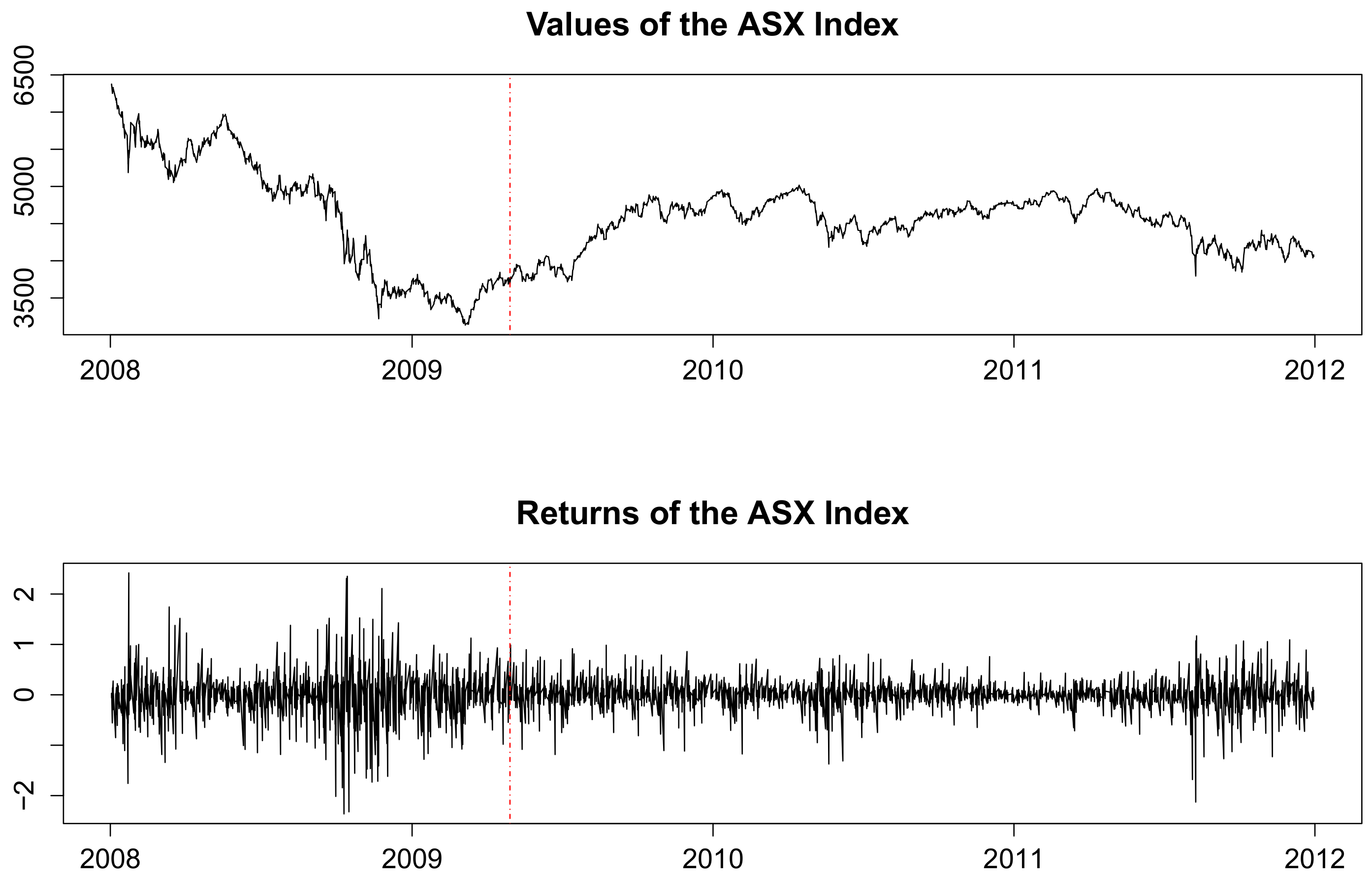
Figure 2.
Hourly closing prices for the selected indexes over the period 1 January 2008 to 31 December 2011.
Figure 2.
Hourly closing prices for the selected indexes over the period 1 January 2008 to 31 December 2011.

Figure 3.
Hourly returns and hourly absolute returns for stock indexes from 1 January 2008 to 31 December 2011.
Figure 3.
Hourly returns and hourly absolute returns for stock indexes from 1 January 2008 to 31 December 2011.
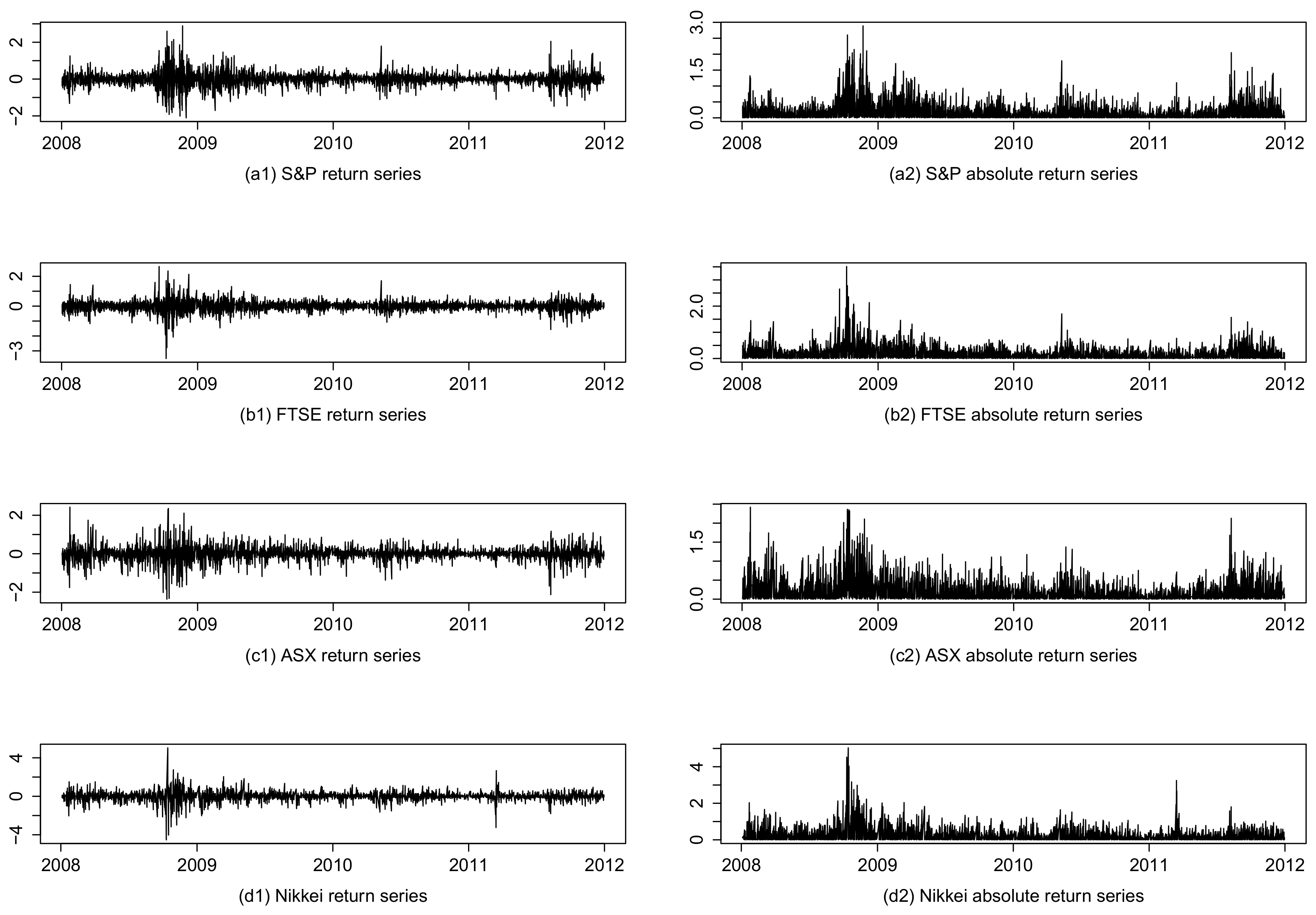
Figure 4.
Autocorrelation functions for the stock indexes.

Figure 5.
Flowchart of the A-HYEGARCH model fitting process.
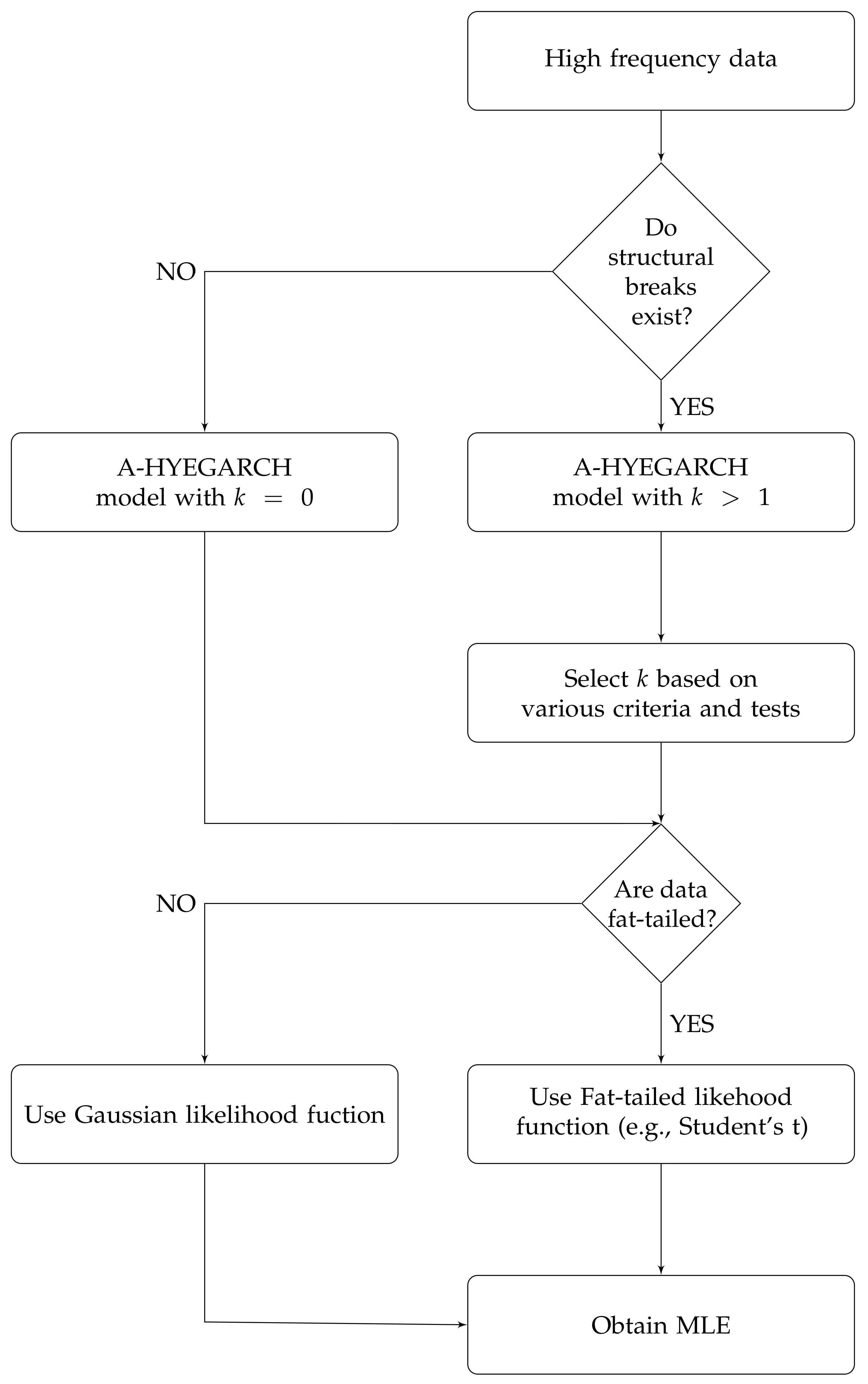
Figure 6.
Identified structural change points.


Table 1.
Simulation results for estimation of A-HYEGARCH models without structural change.
| A-HYEGARCH(0,d,0,0) | A-HYEGARCH(1,d,0,0) | A-HYEGARCH(1,d,1,0) | ||||||||
|---|---|---|---|---|---|---|---|---|---|---|
| T | d | |||||||||
| d = 0.25 | ||||||||||
| 1000 | 0.25 | 0.1825 | 0.4503 | 0.4116 | 0.0591 | 0.3247 | 0.3193 | 0.1032 | 0.2995 | 0.2812 |
| 3000 | 0.25 | 0.1325 | 0.3547 | 0.3290 | 0.0056 | 0.2219 | 0.2218 | 0.0683 | 0.2521 | 0.2427 |
| 5000 | 0.25 | 0.0814 | 0.2788 | 0.2666 | 0.0078 | 0.1925 | 0.1923 | 0.0564 | 0.2017 | 0.1936 |
| d = 0.35 | ||||||||||
| 1000 | 0.35 | 0.0973 | 0.3484 | 0.3345 | 0.0115 | 0.3189 | 0.3187 | 0.0410 | 0.2661 | 0.2629 |
| 3000 | 0.35 | 0.0850 | 0.3021 | 0.2899 | 0.2152 | 0.2146 | 0.0237 | 0.2063 | 0.2049 | |
| 5000 | 0.35 | 0.0764 | 0.2556 | 0.2439 | 0.0208 | 0.1812 | 0.1800 | 0.0287 | 0.1925 | 0.1903 |
| d = 0.45 | ||||||||||
| 1000 | 0.45 | 0.1317 | 0.3592 | 0.3341 | 0.0145 | 0.3221 | 0.3218 | 0.0264 | 0.2816 | 0.2804 |
| 3000 | 0.45 | 0.2506 | 0.2486 | 0.2174 | 0.2139 | 0.2356 | 0.2333 | |||
| 5000 | 0.45 | 0.0289 | 0.2352 | 0.2334 | 0.2113 | 0.2081 | 0.1770 | 0.1770 | ||
Note: This table reports simulation results for the bias, root mean square error (RMSE) and standard error (SE) for estimation of the fractional differencing parameter d from simulations with sample size T = . All the results are based on 500 replications.
Table 2.
Simulation results for estimation of A-HYEGARCH models without structural change.
| A-HYEGARCH(0,d,0,k) | A-HYEGARCH(1,d,0,k) | A-HYEGARCH(1,d,1,k) | ||||||||
|---|---|---|---|---|---|---|---|---|---|---|
| T | d | |||||||||
| k = 1 | ||||||||||
| 1000 | 0.25 | 0.0962 | 0.3182 | 0.3034 | 0.0860 | 0.2971 | 0.2844 | 0.0624 | 0.2757 | 0.2685 |
| 3000 | 0.25 | 0.1122 | 0.2903 | 0.2678 | 0.0220 | 0.2161 | 0.2150 | 0.0557 | 0.2500 | 0.2437 |
| 5000 | 0.25 | 0.0691 | 0.2424 | 0.2324 | 0.0614 | 0.2376 | 0.2295 | 0.0448 | 0.2007 | 0.1957 |
| 1000 | 0.35 | 0.1398 | 0.3331 | 0.3024 | 0.0868 | 0.3136 | 0.3013 | 0.0746 | 0.2967 | 0.2871 |
| 3000 | 0.35 | 0.0724 | 0.2638 | 0.2536 | 0.0082 | 0.2329 | 0.2327 | 0.0226 | 0.2405 | 0.2394 |
| 5000 | 0.35 | 0.0389 | 0.2295 | 0.2262 | 0.0218 | 0.2236 | 0.2225 | 0.0424 | 0.227 | 0.223 |
| 1000 | 0.45 | 0.0612 | 0.3339 | 0.3283 | 0.2799 | 0.2796 | 0.0106 | 0.3063 | 0.3061 | |
| 3000 | 0.45 | 0.0495 | 0.2404 | 0.2352 | 0.0399 | 0.2140 | 0.2103 | 0.2094 | 0.2076 | |
| 5000 | 0.45 | 0.0404 | 0.2502 | 0.2470 | 0.1985 | 0.1942 | 0.1839 | 0.1831 | ||
| k = 2 | ||||||||||
| 1000 | 0.25 | 0.1285 | 0.3632 | 0.3397 | 0.0556 | 0.3060 | 0.3009 | 0.0845 | 0.3006 | 0.2885 |
| 3000 | 0.25 | 0.0613 | 0.2586 | 0.2512 | 0.0868 | 0.2537 | 0.2384 | 0.0597 | 0.2244 | 0.2163 |
| 5000 | 0.25 | 0.1079 | 0.2764 | 0.2545 | 0.0393 | 0.2119 | 0.2082 | 0.0379 | 0.2055 | 0.2019 |
| 1000 | 0.35 | 0.0682 | 0.3070 | 0.2993 | 0.0689 | 0.3105 | 0.3028 | 0.0839 | 0.3054 | 0.2936 |
| 3000 | 0.35 | 0.0777 | 0.2873 | 0.2765 | 0.0289 | 0.2428 | 0.2411 | 0.0090 | 0.2209 | 0.2207 |
| 5000 | 0.35 | 0.0196 | 0.2138 | 0.2129 | 0.0208 | 0.1834 | 0.1822 | 0.1997 | 0.1978 | |
| 1000 | 0.45 | 0.0558 | 0.2911 | 0.2857 | 0.0253 | 0.2925 | 0.2914 | 0.2911 | 0.2911 | |
| 3000 | 0.45 | 0.2205 | 0.2183 | 0.2358 | 0.2255 | 0.2039 | 0.2015 | |||
| 5000 | 0.45 | 0.0354 | 0.2285 | 0.2257 | 0.1992 | 0.1965 | 0.2055 | 0.2032 | ||
| k = 3 | ||||||||||
| 1000 | 0.25 | 0.0630 | 0.3136 | 0.3072 | 0.0126 | 0.3085 | 0.3082 | 0.0718 | 0.3064 | 0.2979 |
| 3000 | 0.25 | 0.0955 | 0.2777 | 0.2608 | 0.0485 | 0.2204 | 0.2150 | 0.0211 | 0.2152 | 0.2142 |
| 5000 | 0.25 | 0.1113 | 0.2720 | 0.2482 | 0.0261 | 0.1948 | 0.1930 | 0.0450 | 0.2047 | 0.1997 |
| 1000 | 0.35 | 0.0825 | 0.2978 | 0.2861 | 0.0554 | 0.2935 | 0.2882 | 0.0275 | 0.2569 | 0.2554 |
| 3000 | 0.35 | 0.0313 | 0.2394 | 0.2374 | 0.2082 | 0.2081 | 0.0234 | 0.2215 | 0.2203 | |
| 5000 | 0.35 | 0.0480 | 0.2161 | 0.2107 | 0.1881 | 0.1880 | 0.1965 | 0.1955 | ||
| 1000 | 0.45 | 0.0785 | 0.3125 | 0.3025 | 0.0245 | 0.2578 | 0.2567 | 0.2840 | 0.2834 | |
| 3000 | 0.45 | 0.0370 | 0.2412 | 0.2383 | 0.0039 | 0.2263 | 0.2263 | 0.2092 | 0.2071 | |
| 5000 | 0.45 | 0.0156 | 0.2065 | 0.2059 | 0.1948 | 0.1944 | 0.2057 | 0.199 | ||
| k = 4 | ||||||||||
| 1000 | 0.25 | 0.0205 | 0.3268 | 0.3262 | 0.0251 | 0.2939 | 0.2928 | 0.0262 | 0.2441 | 0.2427 |
| 3000 | 0.25 | 0.0478 | 0.2362 | 0.2313 | 0.0344 | 0.2197 | 0.217 | 0.0171 | 0.2069 | 0.2061 |
| 5000 | 0.25 | 0.0870 | 0.2153 | 0.1969 | 0.0403 | 0.2196 | 0.2159 | 0.0186 | 0.1894 | 0.1885 |
| 1000 | 0.35 | 0.0970 | 0.3050 | 0.2891 | 0.0488 | 0.2951 | 0.2910 | 0.2698 | 0.2675 | |
| 3000 | 0.35 | 0.0401 | 0.2181 | 0.2144 | 0.2224 | 0.2214 | 0.0132 | 0.2231 | 0.2227 | |
| 5000 | 0.35 | 0.0371 | 0.2076 | 0.2043 | 0.2129 | 0.2125 | 0.0061 | 0.1773 | 0.1772 | |
| 1000 | 0.45 | 0.0352 | 0.2979 | 0.2958 | 0.0130 | 0.2921 | 0.2918 | 0.2639 | 0.2605 | |
| 3000 | 0.45 | 0.0176 | 0.2436 | 0.2430 | 0.0016 | 0.2392 | 0.2392 | 0.2296 | 0.2246 | |
| 5000 | 0.45 | 0.0054 | 0.1920 | 0.1919 | 0.199 | 0.1979 | 0.1930 | 0.1833 | ||
Table 3.
Simulation results for estimation of A-HYEGARCH models with various structural change designs.
Table 3.
Simulation results for estimation of A-HYEGARCH models with various structural change designs.
| A-HYEGARCH(0,0.25,0,k) | A-HYEGARCH (0,0.35,0,k) | A-HYEGARCH (0,0.45,0,k) | ||||||||
|---|---|---|---|---|---|---|---|---|---|---|
| T = 1000 | ||||||||||
| k = 0 | 0.3535 | 0.5499 | 0.4213 | 0.3255 | 0.5169 | 0.4015 | 0.2172 | 0.3772 | 0.3084 | |
| 0.1826 | 0.4724 | 0.4357 | 0.1099 | 0.4546 | 0.4411 | 0.0326 | 0.4370 | 0.4358 | ||
| k = 1 | 0.3116 | 0.5484 | 0.4514 | 0.2937 | 0.5203 | 0.4295 | 0.1997 | 0.4290 | 0.3796 | |
| 0.1444 | 0.5077 | 0.4867 | 0.0254 | 0.4945 | 0.4938 | 0.0075 | 0.4642 | 0.4641 | ||
| k = 2 | 0.3482 | 0.5699 | 0.4512 | 0.2783 | 0.5142 | 0.4324 | 0.1767 | 0.4274 | 0.3891 | |
| 0.1272 | 0.4910 | 0.4743 | 0.0881 | 0.4552 | 0.4466 | 0.0354 | 0.4493 | 0.4479 | ||
| k = 3 | 0.2940 | 0.5650 | 0.4825 | 0.2640 | 0.5124 | 0.4392 | 0.1309 | 0.4399 | 0.4199 | |
| 0.1572 | 0.4703 | 0.4433 | 0.0996 | 0.4902 | 0.4800 | 0.0255 | 0.4268 | 0.4260 | ||
| k = 4 | 0.2927 | 0.5563 | 0.4730 | 0.2772 | 0.5299 | 0.4516 | 0.1504 | 0.4320 | 0.4050 | |
| 0.1383 | 0.4612 | 0.4399 | 0.1023 | 0.4566 | 0.4450 | 0.4456 | 0.4454 | |||
| T = 3000 | ||||||||||
| k = 0 | 0.3694 | 0.5307 | 0.3810 | 0.2030 | 0.4321 | 0.3814 | 0.1799 | 0.4394 | 0.4009 | |
| 0.2198 | 0.4301 | 0.3698 | 0.1766 | 0.4253 | 0.3869 | 0.0178 | 0.3840 | 0.3836 | ||
| k = 1 | 0.3335 | 0.5351 | 0.4185 | 0.1805 | 0.4370 | 0.3980 | 0.1477 | 0.4250 | 0.3985 | |
| 0.1902 | 0.4199 | 0.3744 | 0.1690 | 0.4417 | 0.4081 | 0.0037 | 0.4013 | 0.4013 | ||
| k = 2 | 0.2515 | 0.5254 | 0.4613 | 0.1319 | 0.4408 | 0.4206 | 0.1157 | 0.4276 | 0.4117 | |
| 0.1478 | 0.4251 | 0.3986 | 0.1612 | 0.4377 | 0.4069 | 0.4185 | 0.4172 | |||
| k = 3 | 0.2760 | 0.5224 | 0.4436 | 0.1055 | 0.4372 | 0.4243 | 0.0845 | 0.4490 | 0.4410 | |
| 0.1233 | 0.4190 | 0.4004 | 0.1451 | 0.4376 | 0.4129 | 0.3924 | 0.3918 | |||
| k = 4 | 0.3141 | 0.5100 | 0.4018 | 0.1378 | 0.4490 | 0.4274 | 0.0999 | 0.4360 | 0.4244 | |
| 0.1487 | 0.4327 | 0.4063 | 0.1358 | 0.4503 | 0.4293 | 0.0179 | 0.3866 | 0.3861 | ||
| T = 5000 | ||||||||||
| k = 0 | 0.3010 | 0.4992 | 0.3982 | 0.2359 | 0.4001 | 0.3232 | 0.1932 | 0.3482 | 0.2897 | |
| 0.2740 | 0.4985 | 0.4165 | 0.1021 | 0.4339 | 0.4217 | 0.4230 | 0.4230 | |||
| k = 1 | 0.2707 | 0.4635 | 0.3763 | 0.1845 | 0.3874 | 0.3406 | 0.1092 | 0.3451 | 0.3273 | |
| 0.2359 | 0.4849 | 0.4237 | 0.0745 | 0.4098 | 0.4030 | 0.0178 | 0.4064 | 0.4060 | ||
| k = 2 | 0.2172 | 0.4555 | 0.4004 | 0.1461 | 0.3750 | 0.3454 | 0.0844 | 0.3558 | 0.3456 | |
| 0.2220 | 0.4855 | 0.4318 | 0.0647 | 0.4312 | 0.4263 | 0.4102 | 0.4099 | |||
| k = 3 | 0.2339 | 0.4710 | 0.4088 | 0.1652 | 0.3874 | 0.3504 | 0.0688 | 0.3596 | 0.3530 | |
| 0.2306 | 0.5114 | 0.4564 | 0.0599 | 0.4376 | 0.4335 | 0.4170 | 0.4168 | |||
| k = 4 | 0.2465 | 0.4667 | 0.3962 | 0.1597 | 0.3821 | 0.3471 | 0.0994 | 0.3776 | 0.3642 | |
| 0.2320 | 0.4865 | 0.4277 | 0.0601 | 0.4410 | 0.4369 | 0.4188 | 0.4185 | |||
Note: As for Table 2; but simulations are for three different experiment designs: a single break () and two break points ().
Table 4.
Simulation results for estimation of A-HYEGARCH models with various structural change designs.
Table 4.
Simulation results for estimation of A-HYEGARCH models with various structural change designs.
| A-HYEGARCH(1,0.25,0,k) | A-HYEGARCH(1,0.35,0,k) | A-HYEGARCH(1,0.45,0,k) | ||||||||
|---|---|---|---|---|---|---|---|---|---|---|
| T = 1000 | ||||||||||
| k = 0 | 0.3168 | 0.5238 | 0.4171 | 0.2450 | 0.4563 | 0.3850 | 0.0675 | 0.3473 | 0.3406 | |
| 0.2382 | 0.4394 | 0.3692 | 0.0874 | 0.4139 | 0.4046 | 0.3553 | 0.3501 | |||
| k = 1 | 0.2845 | 0.5447 | 0.4645 | 0.1855 | 0.4896 | 0.4530 | 0.0476 | 0.4180 | 0.4152 | |
| 0.2009 | 0.5057 | 0.4642 | 0.0362 | 0.4689 | 0.4675 | 0.4389 | 0.4288 | |||
| k = 2 | 0.2719 | 0.5385 | 0.4648 | 0.1546 | 0.4915 | 0.4666 | 0.0483 | 0.3951 | 0.3921 | |
| 0.2041 | 0.5037 | 0.4604 | 0.0416 | 0.4506 | 0.4487 | 0.4332 | 0.4235 | |||
| k = 3 | 0.2487 | 0.5415 | 0.4810 | 0.1625 | 0.5043 | 0.4774 | 0.0827 | 0.4107 | 0.4023 | |
| 0.1826 | 0.4776 | 0.4413 | 0.0631 | 0.4456 | 0.4411 | 0.4163 | 0.4004 | |||
| k = 4 | 0.2196 | 0.5318 | 0.4844 | 0.2160 | 0.4839 | 0.4331 | 0.0188 | 0.3960 | 0.3956 | |
| 0.2362 | 0.4964 | 0.4366 | 0.0482 | 0.4512 | 0.4486 | 0.4145 | 0.4067 | |||
| T = 3000 | ||||||||||
| k = 0 | 0.3894 | 0.5265 | 0.3543 | 0.2344 | 0.4246 | 0.3541 | 0.1550 | 0.3503 | 0.3142 | |
| 0.2727 | 0.4818 | 0.3972 | 0.1100 | 0.3826 | 0.3665 | 0.3665 | 0.3665 | |||
| k = 1 | 0.4085 | 0.5493 | 0.3672 | 0.2415 | 0.4327 | 0.3590 | 0.1097 | 0.3715 | 0.3549 | |
| 0.2794 | 0.4753 | 0.3845 | 0.0988 | 0.3920 | 0.3794 | 0.3823 | 0.3822 | |||
| k = 2 | 0.3552 | 0.5362 | 0.4016 | 0.2183 | 0.4360 | 0.3773 | 0.0937 | 0.3846 | 0.3730 | |
| 0.2663 | 0.4796 | 0.3988 | 0.0857 | 0.4149 | 0.4059 | 0.0134 | 0.4038 | 0.4036 | ||
| k = 3 | 0.3755 | 0.5433 | 0.3926 | 0.2237 | 0.4498 | 0.3902 | 0.0933 | 0.3875 | 0.3761 | |
| 0.2550 | 0.4757 | 0.4016 | 0.1052 | 0.4070 | 0.3932 | 0.0236 | 0.3966 | 0.3959 | ||
| k = 4 | 0.3800 | 0.5500 | 0.3976 | 0.2165 | 0.4548 | 0.4000 | 0.0999 | 0.3954 | 0.3826 | |
| 0.2549 | 0.4801 | 0.4068 | 0.0918 | 0.4058 | 0.3953 | 0.0090 | 0.3918 | 0.3917 | ||
| T = 5000 | ||||||||||
| k = 0 | 0.3584 | 0.4842 | 0.3256 | 0.2809 | 0.4373 | 0.3352 | 0.1708 | 0.3463 | 0.3013 | |
| 0.2371 | 0.4271 | 0.3553 | 0.1292 | 0.3670 | 0.3436 | 0.0204 | 0.3727 | 0.3721 | ||
| k = 1 | 0.3300 | 0.4842 | 0.3543 | 0.2433 | 0.4527 | 0.3818 | 0.1689 | 0.3810 | 0.3415 | |
| 0.2062 | 0.4450 | 0.3944 | 0.1190 | 0.3827 | 0.3637 | 0.3818 | 0.3815 | |||
| k = 2 | 0.3327 | 0.4850 | 0.3529 | 0.2369 | 0.4487 | 0.3811 | 0.1843 | 0.3715 | 0.3225 | |
| 0.2106 | 0.4423 | 0.3889 | 0.1163 | 0.3841 | 0.3661 | 0.3971 | 0.3963 | |||
| k = 3 | 0.3129 | 0.4897 | 0.3766 | 0.2487 | 0.4638 | 0.3915 | 0.1586 | 0.3887 | 0.3549 | |
| 0.2000 | 0.4392 | 0.3910 | 0.1086 | 0.3829 | 0.3672 | 0.4106 | 0.4105 | |||
| k = 4 | 0.3246 | 0.4989 | 0.3789 | 0.2783 | 0.4717 | 0.3808 | 0.1723 | 0.3812 | 0.3400 | |
| 0.2129 | 0.4375 | 0.3822 | 0.1054 | 0.3871 | 0.3725 | 0.0118 | 0.4077 | 0.4076 | ||
Note: As for Table 2; but simulations are for three different experiment designs: a single break () and two break points ().
Table 5.
Simulation results for estimation of A-HYEGARCH models with various structural change designs.
Table 5.
Simulation results for estimation of A-HYEGARCH models with various structural change designs.
| A-HYEGARCH(1,0.25,1,k) | A-HYEGARCH(1,0.35,1,k) | A-HYEGARCH(1,0.45,1,k) | ||||||||
|---|---|---|---|---|---|---|---|---|---|---|
| T = 1000 | ||||||||||
| k = 0 | 0.2015 | 0.3644 | 0.3036 | 0.0876 | 0.3218 | 0.3097 | 0.2947 | 0.2897 | ||
| 0.1061 | 0.3118 | 0.2932 | 0.0471 | 0.3628 | 0.3598 | 0.4070 | 0.4004 | |||
| k = 1 | 0.1394 | 0.4135 | 0.3893 | 0.1061 | 0.4132 | 0.3994 | 0.3585 | 0.3524 | ||
| 0.0851 | 0.4208 | 0.4121 | 0.4226 | 0.4225 | 0.4676 | 0.4522 | ||||
| k = 2 | 0.1279 | 0.4429 | 0.4240 | 0.0502 | 0.3949 | 0.3916 | 0.3767 | 0.3641 | ||
| 0.0687 | 0.4108 | 0.4050 | 0.4111 | 0.4107 | 0.4537 | 0.4385 | ||||
| k = 3 | 0.1580 | 0.4299 | 0.3998 | 0.0641 | 0.3929 | 0.3877 | 0.3682 | 0.3587 | ||
| 0.1002 | 0.3902 | 0.3771 | 0.0076 | 0.4107 | 0.4106 | 0.4491 | 0.4327 | |||
| k = 4 | 0.1309 | 0.4400 | 0.4201 | 0.0354 | 0.3789 | 0.3772 | 0.3710 | 0.3676 | ||
| 0.0771 | 0.3557 | 0.3473 | 0.0134 | 0.3838 | 0.3835 | 0.4393 | 0.4114 | |||
| T = 3000 | ||||||||||
| k = 0 | 0.1453 | 0.2613 | 0.2172 | 0.2247 | 0.2238 | 0.2239 | 0.2013 | |||
| 0.0674 | 0.2950 | 0.2873 | 0.2144 | 0.2127 | 0.2745 | 0.2428 | ||||
| k = 1 | 0.0923 | 0.2956 | 0.2808 | 0.2755 | 0.2707 | 0.3017 | 0.2769 | |||
| 0.0108 | 0.3327 | 0.3325 | 0.2863 | 0.2792 | 0.3375 | 0.3020 | ||||
| k = 2 | 0.0869 | 0.3140 | 0.3018 | 0.2892 | 0.2803 | 0.2815 | 0.2614 | |||
| 0.0250 | 0.3499 | 0.3490 | 0.2811 | 0.2633 | 0.3571 | 0.2954 | ||||
| k = 3 | 0.1231 | 0.3323 | 0.3087 | 0.2718 | 0.2583 | 0.3074 | 0.2823 | |||
| 0.0390 | 0.3481 | 0.3459 | 0.2774 | 0.2674 | 0.3350 | 0.2736 | ||||
| k = 4 | 0.1274 | 0.3230 | 0.2968 | 0.2742 | 0.2684 | 0.3065 | 0.2615 | |||
| 0.0231 | 0.3154 | 0.3145 | 0.2545 | 0.2492 | 0.3077 | 0.2750 | ||||
| T = 5000 | ||||||||||
| k = 0 | 0.0580 | 0.2532 | 0.2465 | 0.0357 | 0.2118 | 0.2087 | 0.3114 | 0.3027 | ||
| 0.0589 | 0.2399 | 0.2326 | 0.2661 | 0.2617 | 0.3214 | 0.2871 | ||||
| k = 1 | 0.2476 | 0.2471 | 0.2606 | 0.2594 | 0.3395 | 0.3254 | ||||
| 0.2390 | 0.2388 | 0.2992 | 0.2800 | 0.3711 | 0.3080 | |||||
| k = 2 | 0.2615 | 0.2612 | 0.0018 | 0.2566 | 0.2566 | 0.3426 | 0.3298 | |||
| 0.0018 | 0.2504 | 0.2504 | 0.2995 | 0.2860 | 0.3661 | 0.3102 | ||||
| k = 3 | 0.2656 | 0.2653 | 0.2388 | 0.2371 | 0.3506 | 0.3380 | ||||
| 0.0110 | 0.2405 | 0.2402 | 0.3089 | 0.3002 | 0.3643 | 0.3048 | ||||
| k = 4 | 0.0177 | 0.2624 | 0.2618 | 0.0208 | 0.2587 | 0.2579 | 0.3505 | 0.3364 | ||
| 0.0135 | 0.2550 | 0.2547 | 0.2915 | 0.2856 | 0.3417 | 0.2921 | ||||
Note: As for Table 2; but simulations are for three different experiment designs: a single break () and two break points ().
Table 6.
Summary statistics for the four stock index return series.
| S&P | FTSE | ASX | Nikkei | |
|---|---|---|---|---|
| Panel A: Descriptive statistics | ||||
| Min | ||||
| Max | 2.8884 | 2.6530 | 2.4190 | 5.0316 |
| Mean | ||||
| S.D. | 0.2558 | 0.2312 | 0.2404 | 0.3101 |
| Skew | 0.2627 | |||
| Kurt. | 18.0721 | 22.7123 | 21.2869 | 39.3868 |
| K.S. | 0.0000 | 0.0000 | 0.0000 | 0.0000 |
| J.B. | 0.0000 | 0.0000 | 0.0000 | 0.0000 |
| 0.0000 | 0.0000 | 0.0000 | 0.0000 | |
| Panel B: Pairwise correlations | ||||
| S&P | 0.0476 | 0.0353 | ||
| FTSE | 0.0463 | |||
| ASX | 0.0066 | |||
Note: this table presents the summary statistics for hourly S&P, FTSE, ASX and Nikkei index returns ranging from 1 January 2008 to 31 December 2011. Min is the minimum, Max is the maximum, Mean is the mean, S.D. is the standard deviation, Skew is the skewness, Kurt. is the kurtosis, K.S. is the p-value of Kolmogorov–Smirnov normality test, J.B. is the p-value of Jarque–Bera normality test, is the p-value of the Ljung–Box test for absolute returns at lags 10.
Table 7.
Estimation of FIGARCH, HYGARCH, FIEGARCH and HYEGARCH models for stock indexes.
| d | |||||||||
|---|---|---|---|---|---|---|---|---|---|
| Panel A: S&P | |||||||||
| FIGARCH | 0.0069 | 0.0002 | 0.0482 | 0.9563 | - | 0.9411 | 2.9587 | - | - |
| (0.0013) | 0.0000 | (0.0111) | (0.0028) | (0.0088) | (0.0412) | ||||
| HYGARCH | 0.0071 | 0.0001 | 0.0998 | 0.9541 | 1.0496 | 0.8837 | 2.4009 | - | - |
| (0.0012) | 0.0000 | (0.0195) | (0.0017) | (0.0026) | (0.0160) | (0.0133) | |||
| FIEGARCH | 0.0068 | 0.7963 | - | 0.7405 | 2.5618 | 0.0519 | |||
| (0.0007) | (0.2037) | (0.0122) | (0.0336) | (0.0133) | (0.0150) | (0.0051) | (0.0044) | ||
| HYEGARCH | 0.0069 | 0.7983 | 1.0008 | 0.7294 | 2.5671 | 0.0511 | |||
| (0.0007) | (0.1120) | (0.0121) | (0.0340) | (0.0009) | (0.0131) | (0.0151) | (0.0050) | (0.0044) | |
| Panel B: FTSE | |||||||||
| FIGARCH | 0.0038 | 0.0006 | 0.3015 | 0.8338 | - | 0.5830 | 3.5724 | - | - |
| (0.0014) | (0.0001) | (0.0106) | (0.0040) | (0.0066) | (0.0744) | ||||
| HYGARCH | 0.0038 | 0.0003 | 0.3326 | 0.8287 | 1.0345 | 0.5452 | 3.3689 | - | - |
| (0.0014) | (0.0001) | (0.0117) | (0.0045) | (0.0051) | (0.0072) | (0.0615) | |||
| FIEGARCH | 0.0025 | 2.0009 | 0.5551 | - | 0.9030 | 2.7199 | 0.0840 | ||
| (0.0009) | (0.1899) | (0.0840) | (0.1070) | (0.0126) | (0.0175) | (0.0068) | (0.0082) | ||
| HYEGARCH | 0.0048 | 4.8845 | 0.4221 | 1.0017 | 0.9085 | 3.3806 | 0.0716 | ||
| (0.0009) | (0.1555) | (0.0446) | (0.0523) | (0.0001) | (0.0089) | (0.0419) | (0.0054) | (0.0032) | |
| Panel C: ASX | |||||||||
| FIGARCH | 0.0004 | 0.0957 | 0.9610 | - | 0.8867 | 2.4267 | - | - | |
| (0.0012) | 0.0000 | (0.0103) | (0.0015) | (0.0036) | (0.0148) | ||||
| HYGARCH | 0.0006 | 0.3033 | 0.9435 | 1.1484 | 0.5944 | 2.1465 | - | - | |
| (0.0012) | (0.0001) | (0.0183) | (0.0020) | (0.0060) | (0.0106) | (0.0043) | |||
| FIEGARCH | 0.0016 | 0.9726 | - | 0.9399 | 2.5036 | 0.0947 | |||
| (0.0010) | (0.1440) | (0.0277) | (0.0849) | (0.0161) | (0.0139) | (0.0086) | (0.0112) | ||
| HYEGARCH | 3.1965 | 0.7814 | 1.9430 | 0.9941 | 0.8517 | 2.1654 | 0.0086 | ||
| (0.0015) | (0.2163) | (0.0043) | (0.0593) | (0.0001) | (0.0137) | (0.0042) | (0.0010) | (0.0002) | |
| Panel D: Nikkei | |||||||||
| FIGARCH | 0.0011 | 0.0770 | 0.9462 | - | 0.8637 | 2.2515 | - | - | |
| (0.0013) | (0.0001) | (0.0034) | (0.0004) | (0.0007) | (0.0088) | ||||
| HYGARCH | 0.0009 | 0.1998 | 0.9432 | 1.1550 | 0.6272 | 2.0906 | - | - | |
| (0.0013) | (0.0002) | (0.0056) | (0.0016) | (0.0020) | (0.0019) | (0.0029) | |||
| FIEGARCH | 0.2430 | 0.5857 | 0.1611 | - | 0.7615 | 2.0535 | 0.0028 | ||
| (0.0002) | (0.0810) | (0.0141) | (0.0407) | (0.0045) | (0.0016) | (0.0039) | (0.0001) | ||
| HYEGARCH | 3.4457 | 0.9938 | 0.8002 | 2.1007 | 0.4667 | ||||
| (0.0006) | (0.0934) | (0.0113) | (0.0077) | (0.0001) | (0.0103) | (0.0029) | (0.0278) | (0.0084) | |
Note: this table reports estimates of parameters for the four non-adaptive models, with standard errors presented in parenthesis below corresponding parameter estimates.
Table 8.
Estimation of A-FIGARCH, A-HYGARCH, A-FIEGARCH and A-HYEGARCH models for S&P and FTSE.
| S&P | FTSE | |||||||
|---|---|---|---|---|---|---|---|---|
| A-FIGARCH | A-HYGARCH | A-FIEGARCH | A-HYEGARCH | A-FIGARCH | A-HYGARCH | A-FIEGARCH | A-HYEGARCH | |
| 0.0071 | 0.0071 | 0.0063 | 0.0064 | 0.0036 | 0.0036 | 0.0010 | 0.0040 | |
| (0.0012) | (0.0012) | (0.0004) | (0.0004) | (0.0014) | (0.0014) | (0.0007) | (0.0004) | |
| 0.0019 | 0.0017 | 0.0021 | 0.0026 | 2.0738 | 2.8709 | |||
| 0.0000 | 0.0000 | (0.1658) | (0.2507) | (0.0002) | (0.0001) | (0.3358) | (0.1785) | |
| 0.0441 | 0.0597 | 0.7852 | 0.8150 | 0.4261 | 0.4045 | |||
| (0.0161) | (0.0195) | (0.0088) | (0.0099) | (0.0095) | (0.0096) | (0.0836) | (0.3260) | |
| 0.9514 | 0.9531 | 0.7632 | 0.7648 | 0.3627 | 0.1230 | |||
| (0.0023) | (0.0019) | (0.0289) | (0.0316) | (0.0052) | (0.0050) | (0.0801) | (0.0302) | |
| - | 1.0154 | - | 1.0067 | - | 0.9742 | - | 1.0015 | |
| (0.0023) | (0.0006) | (0.0077) | 0.0000 | |||||
| - | - | -0.1292 | -0.1277 | - | - | |||
| (0.0064) | (0.0056) | (0.0069) | (0.0044) | |||||
| - | - | 0.0353 | 0.0312 | - | - | 0.0688 | 0.0363 | |
| (0.0016) | (0.0015) | (0.0081) | (0.0015) | |||||
| d | 0.9541 | 0.9390 | 0.6313 | 0.5773 | 0.3878 | 0.4219 | 0.8867 | 0.8911 |
| (0.0132) | (0.0156) | (0.0084) | (0.0066) | (0.0074) | (0.0076) | (0.0095) | (0.0053) | |
| 2.5309 | 2.4206 | 2.3700 | 2.4137 | 3.4354 | 3.4410 | 2.7041 | 3.6283 | |
| 0.0000 | (0.0141) | (0.0095) | (0.0106) | (0.0655) | (0.0650) | (0.0170) | (0.0534) | |
| 0.0004 | 0.0019 | 0.0266 | 0.0014 | 0.0024 | ||||
| (0.0001) | 0.0000 | (0.0264) | (0.1067) | (0.0002) | (0.0002) | (0.6054) | (0.1679) | |
| 0.0002 | 0.0004 | 0.2730 | 0.0008 | 0.0014 | 0.0634 | 1.5218 | ||
| (0.0001) | (0.0001) | (0.0219) | (0.0888) | (0.0002) | (0.0002) | (0.3027) | (0.1931) | |
| 0.0003 | 0.0007 | 0.0546 | ||||||
| 0.0000 | (0.0001) | (0.0177) | (0.0735) | (0.0002) | (0.0002) | (0.3092) | (0.1148) | |
| ) | 0.4889 | 0.3969 | ||||||
| 0.0000 | 0.0000 | (0.0170) | (0.0705) | (0.0002) | (0.0002) | (0.3963) | (0.1102) | |
| (0.0001) | 0.0000 | (0.0147) | (0.0621) | (0.0002) | (0.0002) | (0.2118) | (0.0871) | |
| 0.0561 | 0.2460 | 0.0000 | ||||||
| 0.0000 | (0.0001) | (0.0149) | (0.0616) | (0.0002) | (0.0002) | (0.1798) | (0.0878) | |
| 0.0004 | 0.0008 | |||||||
| 0.0000 | (0.0001) | (0.0132) | (0.0549) | (0.0002) | (0.0002) | (0.1530) | (0.0700) | |
| 0.0004 | 0.0004 | 0.0008 | 0.0010 | 0.1948 | 0.2555 | |||
| 0.0000 | 0.0000 | (0.0134) | (0.0584) | (0.0002) | (0.0002) | (0.1440) | (0.0694) | |
| 0.0002 | 0.0004 | 0.0043 | 0.0101 | 0.0003 | 0.0009 | |||
| (0.0001) | 0.0000 | (0.0122) | (0.0518) | (0.0002) | (0.0002) | (0.1365) | (0.0629) | |
| 0.0002 | 0.0002 | 0.0413 | 0.2067 | 0.0001 | 0.0003 | 0.0791 | 0.1247 | |
| (0.0001) | (0.0001) | (0.0125) | (0.0536) | (0.0002) | (0.0002) | (0.1301) | (0.0605) | |
| 0.0002 | 0.0001 | |||||||
| 0.0000 | (0.0001) | (0.0122) | (0.0526) | (0.0002) | (0.0002) | (0.1162) | (0.0566) | |
| 0.0001 | 0.0000 | |||||||
| 0.0000 | 0.0000 | (0.0112) | (0.0495) | (0.0002) | (0.0002) | (0.1096) | (0.0515) | |
| 0.0001 | 0.0255 | 0.1135 | 0.0002 | 0.0000 | 0.0414 | 0.0471 | ||
| 0.0000 | 0.0000 | (0.0111) | (0.0479) | (0.0002) | (0.0002) | (0.1021) | (0.0518) | |
| 0.0001 | 0.0002 | 0.0001 | 0.1722 | 0.1173 | ||||
| (0.0001) | (0.0001) | (0.0112) | (0.0493) | (0.0002) | (0.0002) | (0.1033) | (0.0494) | |
| 0.0001 | 0.0002 | 0.0002 | ||||||
| 0.0000 | (0.0001) | (0.0110) | (0.0490) | (0.0002) | (0.0002) | (0.0934) | (0.0458) | |
| 0.0017 | 0.0021 | 0.0002 | ||||||
| 0.0000 | 0.0000 | (0.0106) | (0.0462) | (0.0001) | (0.0002) | (0.0930) | (0.0468) | |
Note: this table reports estimates of parameters for the four fitted models which all have pairs of trigonometric components in , with standard errors presented in parenthesis below corresponding parameter estimates. The sample data are collected over the period 1 January 2008 to 31 December 2011 for the S&P and FTSE stock indexes, for a total of and observations for each index, respectively.
Table 9.
Estimation of A-FIGARCH, A-HYGARCH, A-FIEGARCH and A-HYEGARCH models for ASX and Nikkei.
| ASX | Nikkei | |||||||
|---|---|---|---|---|---|---|---|---|
| A-FIGARCH | A-HYGARCH | A-FIEGARCH | A-HYEGARCH | A-FIGARCH | A-HYGARCH | A-FIEGARCH | A-HYEGARCH | |
| 0.0000 | 0.0000 | |||||||
| (0.0012) | (0.0012) | (0.0008) | (0.0005) | (0.0012) | (0.0012) | (0.0012) | (0.0011) | |
| 0.0050 | 0.0052 | 3.2308 | 1.3881 | 0.0233 | 0.0199 | 4.2225 | 1.1887 | |
| (0.0002) | (0.0002) | (0.0473) | (0.0454) | (0.0004) | (0.0004) | (0.0569) | (0.0332) | |
| 0.2154 | 0.3350 | 0.9747 | 0.9516 | 0.2056 | 0.2529 | 0.9532 | ||
| (0.0164) | (0.0204) | (0.0003) | (0.0007) | (0.0041) | (0.0061) | (0.0005) | (0.0106) | |
| 0.9118 | 0.9181 | 6.1132 | 7.8885 | 0.8590 | 0.8987 | 4.6251 | ||
| (0.0031) | (0.0028) | (0.0782) | (0.1321) | (0.0013) | (0.0023) | (0.0647) | (0.0003) | |
| - | 1.1447 | - | 1.0143 | - | 1.1554 | - | 2.6064 | |
| (0.0089) | (0.0007) | (0.0035) | (0.0020) | |||||
| - | - | - | - | 0.0222 | ||||
| (0.0013) | (0.0007) | (0.0026) | (0.0571) | |||||
| - | - | 0.0049 | 0.0013 | - | - | 0.0136 | 1.2551 | |
| (0.0001) | 0.0000 | (0.0002) | (0.0455) | |||||
| d | 0.7333 | 0.5422 | 0.2122 | 0.3450 | 0.6393 | 0.5391 | 0.2132 | 0.0653 |
| (0.0085) | (0.0116) | (0.0013) | (0.0014) | (0.0019) | (0.0027) | (0.0014) | (0.0001) | |
| 2.2107 | 2.1345 | 2.0409 | 2.0599 | 2.0984 | 2.0683 | 2.0359 | 2.0090 | |
| (0.0065) | (0.0039) | (0.0011) | (0.0016) | (0.0031) | (0.0021) | (0.0010) | (0.0003) | |
| 0.0020 | 0.0047 | 0.0022 | 0.0050 | 0.0189 | 0.0035 | 0.3229 | ||
| 0.0014 | 0.0022 | 0.0729 | 0.0058 | 0.0047 | 0.5264 | |||
| (0.0002) | (0.0003) | (0.0015) | (0.0473) | (0.0006) | (0.0008) | (0.0032) | (0.0420) | |
| 0.0016 | 0.0049 | |||||||
| (0.0002) | (0.0003) | (0.0014) | (0.0459) | (0.0004) | (0.0007) | (0.0031) | (0.0396) | |
| (0.0002) | (0.0000) | (0.0014) | (0.0465) | (0.0005) | (0.0005) | (0.0030) | (0.0374) | |
| 0.0007 | ||||||||
| (0.0002) | (0.0002) | (0.0014) | (0.0447) | (0.0005) | (0.0006) | (0.0030) | (0.0392) | |
| 0.0015 | 0.0820 | 0.0011 | 0.0028 | 0.1064 | ||||
| (0.0002) | (0.0003) | (0.0014) | (0.0450) | (0.0005) | (0.0006) | (0.0030) | (0.0364) | |
| 0.0013 | 0.0100 | |||||||
| (0.0002) | (0.0003) | (0.0013) | (0.0429) | (0.0006) | (0.0006) | (0.0029) | (0.0388) | |
| 0.0009 | 0.0012 | 0.0002 | 0.0487 | 0.0114 | 0.0084 | 0.0067 | 0.2248 | |
| (0.0002) | (0.0002) | (0.0014) | (0.0454) | (0.0007) | (0.0006) | (0.0029) | (0.0379) | |
| 0.0015 | 0.0009 | 0.0030 | 0.0095 | 0.0055 | 0.1998 | |||
| (0.0002) | (0.0002) | (0.0013) | (0.0432) | (0.0004) | (0.0007) | (0.0028) | (0.0414) | |
| 0.0013 | 0.0015 | 0.0035 | 0.1610 | 0.0037 | 0.0021 | 0.0017 | 0.1843 | |
| (0.0002) | (0.0003) | (0.0013) | (0.0437) | (0.0004) | (0.0005) | (0.0029) | (0.0360) | |
| 0.0012 | 0.0029 | |||||||
| (0.0002) | (0.0003) | (0.0013) | (0.0432) | (0.0007) | (0.0005) | (0.0028) | (0.0381) | |
| 0.0002 | 0.0000 | 0.0029 | 0.1985 | |||||
| (0.0002) | (0.0002) | (0.0013) | (0.0419) | (0.0006) | (0.0007) | (0.0028) | (0.0379) | |
| 0.0000 | 0.0002 | |||||||
| (0.0002) | (0.0002) | (0.0013) | (0.0420) | (0.0005) | (0.0007) | (0.0028) | (0.0392) | |
| 0.0005 | ||||||||
| (0.0002) | (0.0003) | (0.0013) | (0.0437) | (0.0005) | (0.0006) | (0.0028) | (0.0364) | |
| 0.0012 | ||||||||
| (0.0002) | (0.0003) | (0.0013) | (0.0434) | (0.0005) | (0.0006) | (0.0028) | (0.0389) | |
| 0.0058 | 0.0000 | 0.0255 | ||||||
| (0.0002) | (0.0002) | (0.0013) | (0.0410) | (0.0004) | (0.0006) | (0.0027) | (0.0371) | |
Note: as for Table 8; but the underlying sample data correspond to the ASX and Nikkei stock indexes, over the period 1 January 2008 to 31 December 2011 for a total of and observations for each index, respectively.
Table 10.
Summary of diagnostic statistics and evaluation criteria of fitted adaptive models.
| Log-Likelihood | AIC | BIC | ||||
|---|---|---|---|---|---|---|
| Panel A: S&P | ||||||
| A-FIGARCH | 2759.8950 | 17.2735 | 0.3884 | 17.0067 | ||
| A-HYGARCH | 2761.6019 | 18.4937 | 0.4231 | 18.2473 | ||
| A-FIEGARCH | 2862.2593 | 25.0606 | 0.8789 | 24.1713 | ||
| A-HYEGARCH | 2862.9020 | 24.5154 | 0.9294 | 23.6702 | ||
| Panel B: FTSE | ||||||
| A-FIGARCH | 2914.8105 | 29.4395 | 1.8242 | 28.9177 | ||
| A-HYGARCH | 2915.0273 | 30.3156 | 1.8479 | 29.7808 | ||
| A-FIEGARCH | 2979.7400 | 24.6949 | 2.1089 | 24.4607 | ||
| A-HYEGARCH | 3008.1578 | 17.9299 | 2.2100 | 17.9626 | ||
| Panel C: ASX | ||||||
| A-FIGARCH | 3110.6813 | 42.3133 | 4.3910 | 36.6143 | ||
| A-HYGARCH | 3117.5465 | 41.5592 | 4.3769 | 35.9641 | ||
| A-FIEGARCH | 3152.0775 | 68.8288 | 4.2316 | 57.0540 | ||
| A-HYEGARCH | 3152.1061 | 71.1686 | 4.2512 | 58.7924 | ||
| Panel D: Nikkei | ||||||
| A-FIGARCH | 2019.0830 | 63.5469 | 6.8523 | 65.5967 | ||
| A-HYGARCH | 2023.5644 | 77.3598 | 6.9062 | 79.2479 | ||
| A-FIEGARCH | 2032.6590 | 46.9280 | 6.6981 | 49.6358 | ||
| A-HYEGARCH | 2153.8684 | 43.5520 | 6.6087 | 43.9113 | ||
Note: the sample period is from 1 January 2008 to 31 December 2011 for a total of , , and observations for S&P, FTSE, ASX and Nikkei, respectively. ARCH denotes Engle’s Lagrange multiplier test statistics for ARCH effects, denotes the Ljung–Box test statistic for serial correlation in the standardized residuals, denotes the Ljung–Box test statistic for serial correlation in the squared standardized residuals, is the Akaike information criterion and is the Bayesian information criterion. The estimated models are the A-FIGARCH, A-HYGARCH, A-FIEGARCH and A-HYEGARCH.
© 2018 by the authors. Licensee MDPI, Basel, Switzerland. This article is an open access article distributed under the terms and conditions of the Creative Commons Attribution (CC BY) license (http://creativecommons.org/licenses/by/4.0/).
Share and Cite
MDPI and ACS Style
Shi, Y.; Yang, Y. Modeling High Frequency Data with Long Memory and Structural Change: A-HYEGARCH Model. Risks 2018, 6, 26. https://doi.org/10.3390/risks6020026
AMA Style
Shi Y, Yang Y. Modeling High Frequency Data with Long Memory and Structural Change: A-HYEGARCH Model. Risks. 2018; 6(2):26. https://doi.org/10.3390/risks6020026
Chicago/Turabian StyleShi, Yanlin, and Yang Yang. 2018. "Modeling High Frequency Data with Long Memory and Structural Change: A-HYEGARCH Model" Risks 6, no. 2: 26. https://doi.org/10.3390/risks6020026
Note that from the first issue of 2016, this journal uses article numbers instead of page numbers. See further details here.