On Central Branch/Reinsurance Risk Networks: Exact Results and Heuristics

Abstract

Modeling the interactions between a reinsurer and several insurers, or between a central management branch (CB) and several subsidiary business branches, or between a coalition and its members, are fascinating problems, which suggest many interesting questions. Beyond two dimensions, one cannot expect exact answers. Occasionally, reductions to one dimension or heuristic simplifications yield explicit approximations, which may be useful for getting qualitative insights. In this paper, we study two such problems: the ruin problem for a two-dimensional CB network under a new mathematical model, and the problem of valuation of two-dimensional CB networks by optimal dividends. A common thread between these two problems is that the one dimensional reduction exploits the concept of invariant cones. Perhaps the most important contribution of the paper is the questions it raises; for that reason, we have found it useful to complement the particular examples solved by providing one possible formalization of the concept of a multi-dimensional risk network, which seems to us an appropriate umbrella for the kind of questions raised here.

1. Introduction

Multi-dimensional risk networks is an exciting discipline which emerged recently—see for example Kriele and Wolf (2014); (Albrecher and Asmussen 2010, chp. XIII.9). In our paper, a multi dimensional risk network will be modeled by an “upwards skip-free” process $\mathit{X}(t)=(X_0(t),X_1(t),\cdots ,X_I(t))\in \mathcal{S}$. This means, generalizing (Albrecher and Asmussen 2010, chp. XIII.9 Equation (9.1)), that the process may evolve upwards only by drift or diffusion components, and downwards by jumps (modeling catastrophes) or diffusion1. The index set for the network is denoted by $\mathcal{I}=\{0,1,\dots ,I\}$, with the index 0 being reserved for a central branch (CB), if such a branch exists. The process may continue after attempting to overshoot the state space boundary, via various continuation/regulation mechanisms such as reflection, jumping to the interior, etc. One type of overshoot corresponds to the event that a component becomes negative. In such cases, the CB may intervene to reset the negative component to 0. These “bail-out/capital injections” interventions were studied in Avram and Minca (2015, 2017); Avram et al. (2016). Note that more complex “proportional bailouts” and “stop loss bailouts”, which bring the process to an interior point of the state space, have been recently introduced in Salah and Garrido (2017).

We introduce below a new reinsurance/central branch (CB) network model which combines the bail-out model of Avram and Minca (2015, 2017); Avram et al. (2016) with an older model studied in Avram et al. (2006, 2008a, 2008b); Azcue et al. (2016); Badescu et al. (2011); Badila et al. (2014) involving proportional interventions contributed continuously by the CB to each claim of the subsidiaries. The motivation is to investigate how a CB should combine “distress bail-outs” with continuous risk-sharing of the type used in reinsurance, and in particular with the simplest proportional reinsurance, which leads sometimes to exact solutions. As a bonus, it turned out that a problem which could not be solved exactly in our first papers on the bail-out model became solvable under the combined model, once sufficient proportional reinsurance is added—see Section 5.

This paper is organized as follows. Some background on general risk networks is provided in Section 2. Section 3 introduces a new central branch network model, which unifies the previous “bail-out” model Avram and Minca (2015, 2017); Avram et al. (2016) and the proportional reinsurance model of Avram et al. (2006, 2008a, 2008b); Badescu et al. (2011). A similar model has been studied recently by Boxma et al. (2016) (after the completion of our work)—see also Boxma et al. (2017a, 2017b) for related ideas.

Section 4 revisit known results of Avram et al. (2006, 2008b); Badescu et al. (2011); Badila et al. (2014), notably the concept of invariant cone, which is at the basis of all currently known exact results on proportional reinsurance. The general approach is to obtain an integro-differential equation, and then an algebraic Riemann-Hilbert equation for the Laplace transform of the density of the time to ruin. This Laplace transform, already calculated in Badila et al. (2014), is rederived heuristically in Section 4.3 using the famous cancelation of singularity technique. These sections serve to ease the way into the more difficult situation encountered in Section 5, for our new CB model.

In Section 5, we tackle the first particular case of our new CB model. Here we obtain the Riemann-Hilbert equation for the Laplace transform for a network where both bailouts and proportional reinsurance are present. An explicit result is offered, modulo establishing the fact that the singularity curve is removable, which is left for future work. This section illustrates the utility of our new combined model, since without adding sufficient proportional reinsurance, the Laplace transform could not be obtained analytically in the previous papers Avram and Minca (2015, 2017); Avram et al. (2016).

In Section 6, we turn to the different issue of optimizing dividends. We provide a heuristic dynamic valuation index for general risk networks, based on recent work of Azcue et al. (2016). This section is included to illustrate the fact that heuristics may also contribute, together with numerical methods, to unravel the mysteries of multi-dimensional risk networks, and the potential of applying the already available one and two-dimensional tools for managing multi-dimensional CB networks.

2. General Background on Risk Networks

Let ${\tau }_i(u_i)=inf\{t\ge 0:X_i(t)<0|X_i(0)=u_i\},i=0,1,\cdots ,I$ denote the ruin time of $X_i$ when isolated from the network. There are several ways to define ruin sets ${\mathcal{S}}^c={\mathbb{R}}^{I+1}\backslash \mathcal{S}$ that are of interest for the study of risk networks Chan et al. (2003); Hult and Lindskog (2006); Li et al. (2015):

• The first time when (at least) one insurance company is ruined is given by

  $$\begin{array}{cc}\hfill {\tau }_{\mathrm{or}}& ={\tau }_{\min }:=\underset{i\in \mathcal{I}}{min}{\tau }_i\hfill \\ & =inf\{t\ge 0:\mathit{X}(t)\notin {\mathbb{R}}_{++\dots +}\}\hfill \\ & =inf\{t\ge 0:X_0(t)<0,\mathrm{or}{X}_1(t)<0,\dots ,\mathrm{or}{X}_I(t)<0\}.\hfill \end{array}$$

  (1)
• The first time when all the insurance companies experience simultaneous ruin is denoted by

  $${\tau }_{\mathrm{all}}={\tau }_{\max }:=inf\{t\ge 0:\mathit{X}(t)\in {\mathbb{R}}_{--\dots -}\}=inf\{t\ge 0:max{X}_i(t)<0\}.$$

  (2)
• The first time when the sum of the insurance companies $X_{+}(t)={\sum }_{i\in \mathcal{I}}{X}_i(t)$ is ruined is called

  $${\tau }_{\mathrm{sum}}:=inf\{t\ge 0:X_{+}(t)<0\}.$$
• A general class of insolvency sets was introduced in Hult and Lindskog (2006); Li et al. (2015) (inspired by the “bid-ask matrices” of Kabanov and Safarian (2009); Kabanov (1999)). The insolvency set $R_{\mathit{\omega }}=R_{{\omega }_0,{\omega }_1,\cdots ,{\omega }_I}$ is the set where it is impossible to cover the total negative position using fractions bounded by ${\omega }_i\in [0,1]$, out of the positive positions2

  $$\begin{array}{c}\hfill R_{\mathit{\omega }}=\{\mathit{u}:\sum _{i\in \mathcal{I}}{\omega }_i{(u_i)}_{+}<\sum _{i\in \mathcal{I}}{(-u_i)}_{+}\}.\end{array}$$

  (3)
  Correspondingly, we introduce

  $${\tau }_{\mathit{\omega }}=inf\{t\ge 0:\mathit{X}(t)\in R_{\mathit{\omega }}\}.$$
  When $\mathit{\omega }=\omega \mathbf{1}$ we use the notation $R_{\omega }$.

Example 1.

For $\mathit{\omega }=\mathbf{1}=(1,1,\cdots ,1)$, all transfers are allowed without restrictions and ${\tau }_{\mathbf{1}}={\tau }_{\mathrm{sum}}$, while for $\mathit{\omega }=\mathbf{0}=(0,0,\cdots ,0)$, no transfer is allowed and ${\tau }_{\mathbf{0}}={\tau }_{\mathrm{or}}$.

Depending on the type or ruin set chosen, the ultimate/perpetual ruin probabilities will be denoted by

$$\begin{array}{c}{\mathrm{\Psi }}_{\mathrm{or}}(\mathit{u})=P_{\mathit{u}}\left[{\tau }_{\mathrm{or}}<\infty \right],{\mathrm{\Psi }}_{\mathrm{all}}(\mathit{u})\cdots ,{\mathrm{\Psi }}_{\mathrm{sum}}\cdots ,{\mathrm{\Psi }}_{\mathit{\omega }}(\mathit{u})\cdots .\end{array}$$

(4)

Remark 1.

For dependent models, exact computation of these ruin probabilities, with the exception of ${\mathrm{\Psi }}_{\mathrm{sum}},$ is impossible or quite challenging—see Avram et al. (2007); Cai and Li (2005); Chan et al. (2003); Li et al. (2007); Hu and Jiang (2013). However, in the case of processes with independent components,

$$\begin{array}{c}{\mathrm{\Psi }}_{\mathrm{and}}(u_1,u_2):=P[{\tau }_1(u_1)<\infty ,{\tau }_2(u_2)<\infty ]={\mathrm{\Psi }}_1(u_1){\mathrm{\Psi }}_2(u_2),\hfill \\ {\mathrm{\Psi }}_{\mathrm{or}}={\mathrm{\Psi }}_1(u_1)+{\mathrm{\Psi }}_2(u_2)-{\mathrm{\Psi }}_1(u_1){\mathrm{\Psi }}_2(u_2).\hfill \end{array}$$

In terms of bounds of the ruin probabilities (4), one may easily verify that:

$$\begin{array}{c}{\mathrm{\Psi }}_{\mathrm{all}}(u_1,u_2)\le {\mathrm{\Psi }}_{\mathrm{and}}(u_1,u_2)={\mathrm{\Psi }}_1(u_1)+{\mathrm{\Psi }}_2(u_2)-{\mathrm{\Psi }}_{\mathrm{or}}(u_1,u_2)\hfill \\ \le {\mathrm{\Psi }}_{\mathrm{sum}}(u_1,u_2)\le {\mathrm{\Psi }}_{\mathrm{or}}(u_1,u_2).\hfill \end{array}$$

Furthermore, under positive association (present in common shocks models), it holds that (Cai and Li 2005, Equation (4.1))

$$\begin{array}{c}{\mathrm{\Psi }}_{\mathrm{or}}(u_1,u_2)\le {\mathrm{\Psi }}_1(u_1)+{\mathrm{\Psi }}_2(u_2)-{\mathrm{\Psi }}_1(u_1){\mathrm{\Psi }}_2(u_2).\end{array}$$

Two more sophisticated characteristics of a risk network are:

• The Gerber-Shiu/severity of ruin function induced by a ruin time $\tau$:

  $$\begin{array}{c}{S}_q(\mathit{u},\mathit{\theta }):=E_{\mathit{u}}\left[e^{-q\tau +<\mathit{\theta },\mathit{X}(\tau )>};\tau <\infty \right].\hfill \end{array}$$

  (5)
• The combined optimal discounted dividends until ruin:

  $$\begin{array}{c}{V}^F(\mathit{u}):=\underset{\pi =(R_0,R_1,\cdots ,R_I)}{sup}{E}_{\mathit{u}}{\int }_0^{\tau }{e}^{-qt}\left(\sum _{i=0}^{I}d{R}_i(t)\right),\end{array}$$

  (6)

  induced by a ruin time $\tau$, where $R_i$ denote the nonnegative cumulative dividends/consumption/ benefits processes of the i-th branch.
  This functional may be used, following the ideas of De Finetti (1957) and Miller and Modigliani (1961), to evaluate a network of collaborating companies, i.e., assign a numeric value to its performance, by using an approximation inspired by recent (yet unproved) results of Azcue et al. (2016)—see Section 6. Once this heuristic approximation for the value of the collaborating network is computed, one may compare it with the sums of the values of its components (defined analogously, using individual ruin times in the absence of interactions), and decide whether the existence of the collaboration is justified, as opposed to severing the connections between the subsidiaries.

Some major results for multi-dimensional risk network are:

• The Pollaczek-Khinchine type formula for ${\overline{\mathrm{\Psi }}}_{\mathrm{or}}(\mathit{u})$ provided in the foundational paper Chan et al. (2003).
• The asymptotic treatment of ruin probabilities for conic insolvency sets, assuming regularly varying tails—see Hult and Lindskog (2006).
• Optimizing “decoupled” objectives like total time “in the red”—see Loisel (2005) and asymptotic objectives like “orange time”—see Liu and Woo (2014).

Naturally, since multi-dimensional first passage problems are considerably harder than one dimensional ones, exact formulas for (5) and (6) will only be available occasionally in two-dimensional cases, where complex analysis may come to rescue. Nevertheless, we believe that the few low-dimensional exact results that are already available may provide interesting tools for managing multi-dimensional risk networks.

3. A Bail-Out + Reinsurance Central Branch Risk Network Model

Definition 1.

A central branch (CB) risk network $\mathit{X}(t)=(X_0(t),X_1(t),\cdots ,X_I(t))$ is formed from:

1. 

Several subsidiaries $X_i(t),i=1,\dots ,I$, with downward jumps, which must be kept in certain “solvability regions” by bail-outs from a central branch $X_0(t)$, or be liquidated otherwise. For example, they might need to be maintained above certain prescribed levels $o_i$. For other possible solvability regions, see Section 1.

We will denote by ${\tau }_{i,j},i\in \{1,\dots ,I\},j\in \{1,2,\dots \}$ the j-th intervention time on the i-th subsidiary, to be referred from now on as bailout time.

2. 

The reserve of the CB is a process with downward jumps denoted by $X_0(t)$ in the absence of subsidiaries, and by $X(t)$ after subtracting the bailouts. The ruin time

$$\tau ={\tau }_0^{-}=inf\{t\ge 0:X(t)<0\}$$

causes the ruin of the whole network and leads to a severe penalty.

3. 

The CB must also cover a certain proportion ${\overline{\alpha }}_i=1-{\alpha }_i$ of each claim $C_{i,j}$ of subsidiary i, leaving the subsidiary to pay only ${\alpha }_i{C}_{i,j}$, where ${\alpha }_i\in [0,1]$ are called proportional reinsurance retention levels.

Remark 2.

For a CB network, the bail-out boundaries (for example $u_i=o_i,i=1,\dots ,I$) are reflecting and $u_0\le 0$ is absorbing.

Remark 3.

Both the bail-out times ${\tau }_{i,j},i,j\ge 1$ and the ruin time τ could be replaced by other stopping times such as the Parisian (“soft”) stopping time Albrecher et al. (2016); Avram and Zhou (2016); Avram et al. (2018) or the draw-down (Azema-Yor) stopping time

$${\tau }_{\xi }:=inf\{t\ge 0:X(t)\le \xi \underset{0\le s\le t}{sup}X(s)\},$$

where $\xi \in (0,1)$ is a fixed constant.

Here is one example of process falling under the CB umbrella:

Example 2.

Consider a Cramér-Lundberg subsidiary process $X_1=u_1+c_{1}t-{\alpha }_{1}C(t),$ which shares with the CB, in some proportions to be optimized, the common liability process C. It is also assumed that the central branch $X_0$ has an additional independent dedicated liability $C_0$. In addition, the CB must bail out the subsidiary whenever it becomes negative. The cumulative bailouts will be denoted by $Z(t)$. Assuming the CB pays a total of $k>1$ Euros for each bailout Euro (k is sometimes called the proportional transaction cost), the two companies will satisfy:

$$\begin{array}{c}\left\{\begin{array}{c}{X}_1(t)=u_1+c_{1}t-{\alpha }_{1}C(t)+Z(t)\hfill \\ X(t)=u_0+c_{0}t-(1-{\alpha }_1)C(t)-C_0(t)-kZ(t)\hfill \end{array}\right.\hfill \end{array}$$

(7)

$$C(t)=\sum _{i=1}^{N_{\lambda }(t)}{C}_i,C_0(t)=\sum _{i=1}^{N_{{\lambda }_0}(t)}{C}_{i,0}.$$

If bailouts occur only when $X_1(t)\ne 0$, and this company is always reset to 0, then $Z(t)$ is the so-called “minimal Skorohod reflection process necessary to keep $X_1(t)$ nonnegative”, a nondecreasing process satisfying $X_1(t)\ge 0,{\int }_0^t{X}_1(t)dZ(t)=0$ (i.e., $Z(t)$ only “pushes up” when $X_1(t)=0$). The common liability process $C(t)$, as well as the dedicated liability process $C_0(t)$ are assumed here to be compound Poisson, with Poisson intensities denoted by $\lambda ,{\lambda }_0$.

Remark 4.

The compound Poisson models and independence assumption make sense when the CB is itself an insurance company. Mathematically, this example illustrates one of the main difficulties of dealing with general CB risk networks: the fact that the bailout and the common liability are typically not independent. This makes $X(t)$ a non-standard Sparre-Andersen risk process.

Remark 5.

This example can be generalized by adding a Brownian motion to $X(t),$ as an approximation of the aggregate net flow due to several other subsidiaries. In that case, $X(t)$ is a perturbed non-standard Sparre-Andersen risk process Frostig (2008); Li et al. (2009); Zhang et al. (2013).

Example 3.

A notable exception to the issue of dependence is the case of exponential claims. Taking ${\alpha }_1=1,$ ${\lambda }_0=0$ and $\mathcal{L}(C_i)=Exp(\mu )$ in (7) makes $X(t)$ a Sparre-Andersen process with exponential claims, independent of the inter-arrival times ${\tau }_j,j=1,\dots ,n,\dots$, which are descending ladder times of $X_1$. The Laplace transform of the density of ${\tau }_j$ satisfies a Kendall-Takacs functional equation, which may even be inverted explicitly, by Lagrange-Burmann inversion, resulting in the so-called Takacs series. Even more efficient are Padé approximations of the bail-out time—see Avram and Minca (2015, 2017).

The case of phase-type claims is not straightforward—see Avram et al. (2016), and computing other risk measures for $X(t)$, like expected dividends before ruin, is even more challenging. One possibility is using an approximation approach, based on replacing the exact joint law of $({\tau }_1,X({\tau }_1))$ by a phase-type approximation—see Avram (2017).

Example 4.

Suppose now that ${\lambda }_0>0$, ${\alpha }_1=1$, and $\mathcal{L}(C_j)=Exp(\mu )$ in (7). Then $X(t)$ is a Sparre-Andersen process with exponential claims, with a spectrally negative perturbation Frostig (2008); Li et al. (2009); Zhang et al. (2013). In this case, quantities of interest such as ruin probabilities and expected dividends may be expressed in terms of the roots of a generalized Lundberg equation , and this continues to be the case when $X_0(t)$ includes a Brownian perturbation, which may approximate an aggregate net flow of several subsidiaries.

4. Laplace Transform for the “or”-Ruin Probability of a Proportional Reinsurer with a Dedicated Spectrally Negative Liability

We consider (7) in the absence of crisis bailouts, when the model reduces to:

$$\begin{array}{c}{X}_1(t):=u_1+c_{1}t-{\alpha }_{1}C(t),\hfill \\ X_0(t):=u_0+c_{0}t-{\alpha }_{0}C(t)-C_0(t),\hfill \end{array}$$

where ${\alpha }_0+{\alpha }_1=1$.

Recall that we restrict to the case when the liabilities $C(t)$ and $C_0(t)$ are both compound Poisson, with respective intensities denoted by ${\lambda }_c,{\lambda }_0$, respective jump densities denoted by $f_c,f_0$, and Lévy densities denoted by ${\nu }_c(x)dx$ and ${\nu }_0(x)dx$, respectively. For $j=0,1$, let

$${\tau }_j={\tau }_j(u)=inf\{t\ge 0:X_j(t)<0\},{\mathrm{\Psi }}_j(u)=P({\tau }_j<\infty |X_j(0)=u),{\overline{\mathrm{\Psi }}}_j(u)=P({\tau }_j=\infty |X_j(0)=u).$$

We will denote the “or” time to ruin by

$$\tau ={\tau }_1\wedge {\tau }_0,$$

and write $\tau (u_1,u_2)$ for $\tau$ with fixed initial conditions.

In this section, we will obtain the Laplace transform of the density of $\tau$

$${\varphi }_{\delta }(u_1,u_0):=E[e^{-\delta \tau }{\mathbf{1}}_{(\tau <\infty )}|X_1(0)=u_1,X_0(0)=u_0]=P[\tau <{\mathcal{E}}_{\delta }|X_1(0)=u_1,X_0(0)=u_0],$$

(8)

where ${\mathcal{E}}_{\delta }$ is an independent exponential r.v. with rate $\delta$. This includes as a particular case the eventual “or” ruin probability ${\varphi }_0(u_1,u_0)=E[{\mathbf{1}}_{(\tau <\infty )}|X_1(0)=u_1,X_0(0)=u_0]:=\mathrm{\Psi }(u_1,u_0)$.

4.1. Integro-Differential Equation

Theorem 1.

The Laplace transform (8) satisfies

$$\begin{array}{ccc}\hfill ({\lambda }_c+{\lambda }_0+\delta ){\varphi }_{\delta }(u_1,u_0)& =& c_1\frac{\partial }{\partial u_1}{\varphi }_{\delta }(u_1,u_0)+c_0\frac{\partial }{\partial u_0}{\varphi }_{\delta }(u_1,u_0)\hfill \\ & & +{\lambda }_0{\int }_0^{u_0}{\varphi }_{\delta }(u_1,u_0-x)f_0(x)dx+{\lambda }_0{\overline{F}}_0(u_0)\hfill \\ & & +{\lambda }_c{\int }_0^{\frac{u_1}{{\alpha }_1}\wedge \frac{u_0}{{\alpha }_0}}{\varphi }_{\delta }(u_1-{\alpha }_{1}x,u_0-{\alpha }_{0}x)f_c(x)dx+{\lambda }_c{\overline{F}}_c\left(\frac{u_1}{{\alpha }_1}\wedge \frac{u_0}{{\alpha }_0}\right),\hfill \end{array}$$

(9)

where ${\overline{F}}_c(x)={\int }_x^{\infty }{f}_c(y)dy$ and ${\overline{F}}_0(x)={\int }_x^{\infty }{f}_0(y)dy$ are the survival functions associated with the densities $f_c$ and $f_0$.

Proof. 

Conditioning on all the possible outcomes during the time interval $(0,h)$ as in Avram et al. (2008b), we obtain

$$\begin{array}{ccc}\hfill {\varphi }_{\delta }(u_1,u_0)& =& e^{-{\lambda }_{c}h-{\lambda }_{0}h-\delta h}{\varphi }_{\delta }(u_1+c_{1}h,u_0+c_{0}h)\hfill \\ & & +e^{-{\lambda }_{c}h}{\int }_0^h{\lambda }_0{e}^{-{\lambda }_{0}t-\delta t}{\int }_0^{u_0+c_{0}t}{\varphi }_{\delta }(u_1+c_{1}t,u_0+c_{0}t-x)f_0(x)dxdt\hfill \\ & & +e^{-{\lambda }_{c}h}{\int }_0^h{\lambda }_0{e}^{-{\lambda }_{0}t-\delta t}{\int }_{u_0+c_{0}t}^{\infty }{f}_0(x)dxdt\hfill \\ & & +e^{-{\lambda }_{0}h}{\int }_0^h{\lambda }_c{e}^{-{\lambda }_{c}t-\delta t}{\int }_0^{\frac{(u_1+c_{1}t)}{{\alpha }_1}\wedge \frac{(u_0+c_{0}t)}{{\alpha }_0}}{\varphi }_{\delta }(u_1+c_{1}t-{\alpha }_{1}x,u_0+c_{0}t-{\alpha }_{0}x)f_c(x)dxdt\hfill \\ & & +e^{-{\lambda }_{0}h}{\int }_0^h{\lambda }_c{e}^{-{\lambda }_{c}t-\delta t}{\int }_{\frac{(u_1+c_{1}t)}{{\alpha }_1}\wedge \frac{(u_0+c_{0}t)}{{\alpha }_0}}^{\infty }{f}_c(x)dxdt.\hfill \end{array}$$

(10)

Differentiating both sides of (10) w.r.t. h and then letting $h\to 0$, we obtain the desired result. ☐

4.2. A Riemann-Hilbert Equation for the Laplace Transform

From (9), we will obtain an equation for the two-dimensional Laplace transform

$$\begin{array}{c}\mathcal{L}{\varphi }_{\delta }(s_1,s_0):={\int }_0^{\infty }{\int }_0^{\infty }{e}^{-s_1{u}_1-s_0{u}_0}{\varphi }_{\delta }(u_1,u_0)d{u}_{1}d{u}_0.\end{array}$$

Taking transform of the first four terms in (9) is straightforward:

$$\begin{array}{cc}\hfill \mathcal{L}\frac{\partial }{\partial u_1}{\varphi }_{\delta }(u_1,u_0)& =s_1\mathcal{L}{\varphi }_{\delta }(s_1,s_0)-{\int }_0^{\infty }{e}^{-s_0{u}_0}{\varphi }_{\delta }(0,u_0)d{u}_0,\hfill \\ \hfill \mathcal{L}\frac{\partial }{\partial u_0}{\varphi }_{\delta }(u_1,u_0)& =s_0\mathcal{L}{\varphi }_{\delta }(s_1,s_0)-{\int }_0^{\infty }{e}^{-s_1{u}_1}{\varphi }_{\delta }(u_1,0)d{u}_1,\hfill \\ \hfill \mathcal{L}{\int }_0^{u_0}{\varphi }_{\delta }(u_1,u_0-x)f_0(x)dx& =\mathcal{L}{\varphi }_{\delta }(s_1,s_0){\widehat{f}}_0(s_0),\hfill \\ \hfill \mathcal{L}{\overline{F}}_0(u_0)& =\frac{1-{\widehat{f}}_0(s_0)}{s_0{s}_1},\hfill \end{array}$$

where for any function g, we denote its one-dimensional Laplace transform by $\widehat{g}(s)={\int }_0^{\infty }{e}^{-sx}g(x)dx$.

For the fifth term we change the order of integration:

$$\begin{array}{cc}& {\int }_0^{\infty }{\int }_0^{\infty }{e}^{-s_1{u}_1-s_0{u}_0}{\int }_0^{\frac{u_1}{{\alpha }_1}\wedge \frac{u_0}{{\alpha }_0}}{\varphi }_{\delta }(u_1-{\alpha }_{1}x,u_0-{\alpha }_{0}x)f_c(x)dxd{u}_{1}d{u}_0\hfill \\ =& {\int }_0^{\infty }{e}^{-({\alpha }_1{s}_1+{\alpha }_0{s}_0)x}{\int }_{{\alpha }_{0}x}^{\infty }{\int }_{{\alpha }_{1}x}^{\infty }{e}^{-s_1(u_1-{\alpha }_{1}x)-s_0(u_0-{\alpha }_{0}x)}{\varphi }_{\delta }(u_1-{\alpha }_{1}x,u_0-{\alpha }_{0}x)d{u}_{1}d{u}_0{f}_c(x)dx\hfill \\ =& \mathcal{L}{\varphi }_{\delta }(s_1,s_0){\widehat{f}}_c({\alpha }_1{s}_1+{\alpha }_0{s}_0).\hfill \end{array}$$

Finally, for the sixth term in (9) we split the domain

$$\begin{array}{cc}& {\int }_0^{\infty }{\int }_0^{\infty }{e}^{-s_1{u}_1-s_0{u}_0}{\overline{F}}_c\left(\frac{u_1}{{\alpha }_1}\wedge \frac{u_0}{{\alpha }_0}\right)d{u}_{1}d{u}_0\hfill \\ =& {\int }_0^{\infty }{\int }_0^{\frac{u_0{\alpha }_1}{{\alpha }_0}}{e}^{-s_1{u}_1-s_0{u}_0}{\overline{F}}_c(u_1/{\alpha }_1)d{u}_{1}d{u}_0+{\int }_0^{\infty }{\int }_{\frac{u_0{\alpha }_1}{{\alpha }_0}}^{\infty }{e}^{-s_1{u}_1-s_0{u}_0}{\overline{F}}_c(u_0/{\alpha }_0)d{u}_{1}d{u}_0\hfill \\ =& \frac{1}{s_0}{\int }_0^{\infty }{e}^{-s_1{u}_1-s_0{\alpha }_0{u}_1/{\alpha }_1}{\overline{F}}_c(u_1/{\alpha }_1)d{u}_1+\frac{1}{s_1}{\int }_0^{\infty }{e}^{-s_0{u}_0-s_1{\alpha }_1{u}_0/{\alpha }_0}{\overline{F}}_c(u_0/{\alpha }_0)d{u}_0\hfill \\ =& \frac{1-{\widehat{f}}_c({\alpha }_1{s}_1+{\alpha }_0{s}_0)}{{\alpha }_1{s}_1+{\alpha }_0{s}_0}\left(\frac{{\alpha }_1}{s_0}+\frac{{\alpha }_0}{s_1}\right)=\frac{1-{\widehat{f}}_c({\alpha }_1{s}_1+{\alpha }_0{s}_0)}{s_1{s}_0}.\hfill \end{array}$$

Putting this together we obtain

$$\begin{array}{ccc}\hfill ({\lambda }_c+{\lambda }_0+\delta )\mathcal{L}{\varphi }_{\delta }(s_1,s_0)& =& c_1{s}_1\mathcal{L}{\varphi }_{\delta }(s_1,s_0)-c_1{\int }_0^{\infty }{e}^{-s_0{u}_0}{\varphi }_{\delta }(0,u_0)d{u}_0\hfill \\ & & +c_0{s}_0\mathcal{L}{\varphi }_{\delta }(s_1,s_0)-c_0{\int }_0^{\infty }{e}^{-s_1{u}_1}{\varphi }_{\delta }(u_1,0)d{u}_1\hfill \\ & & +{\lambda }_0\frac{1-{\widehat{f}}_0(s_0)}{s_1{s}_0}+{\lambda }_0\mathcal{L}{\varphi }_{\delta }(s_1,s_0){\widehat{f}}_0(s_0)\hfill \\ & & +{\lambda }_c\mathcal{L}{\varphi }_{\delta }(s_1,s_0){\widehat{f}}_c({\alpha }_1{s}_1+{\alpha }_0{s}_0)+{\lambda }_c\frac{1-{\widehat{f}}_c({\alpha }_1{s}_1+{\alpha }_0{s}_0)}{s_1{s}_0},\hfill \end{array}$$

which is restated as the following theorem.

Theorem 2.

The two-dimensional Laplace transform of ${\varphi }_{\delta }$ satisfies the Riemann-Hilbert equation with three unknowns

$$\begin{array}{c}\mathcal{L}{\varphi }_{\delta }(s_1,s_0)\hfill \\ =\frac{c_1{\int }_0^{\infty }{e}^{-s_0{u}_0}{\varphi }_{\delta }(0,u_0)d{u}_0+c_0{\int }_0^{\infty }{e}^{-s_1{u}_1}{\varphi }_{\delta }(u_1,0)d{u}_1-{\lambda }_0\frac{1-{\widehat{f}}_0(s_0)}{s_1{s}_0}-{\lambda }_c\frac{1-{\widehat{f}}_c({\alpha }_1{s}_1+{\alpha }_0{s}_0)}{s_1{s}_0}}{c_1{s}_1+c_0{s}_0-({\lambda }_c+{\lambda }_0+\delta )+{\lambda }_c{\widehat{f}}_c({\alpha }_1{s}_1+{\alpha }_0{s}_0)+{\lambda }_0{\widehat{f}}_0(s_0)}\hfill \\ =\frac{c_1{\widehat{\varphi }}_{\delta }(0,s_0)+c_0{\widehat{\varphi }}_{\delta }(s_1,0)+\frac{\kappa (s_1,s_0)-c_0{s}_0-c_1{s}_1}{s_1{s}_0}}{\kappa (s_1,s_0)-\delta }=\frac{1}{s_0{s}_1}-\frac{c_1(\frac{1}{s_0}-{\widehat{\varphi }}_{\delta }(0,s_0))+c_0(\frac{1}{s_1}-{\widehat{\varphi }}_{\delta }(s_1,0))-\frac{\delta }{s_1{s}_0}}{\kappa (s_1,s_0)-\delta },\hfill \end{array}$$

(11)

where we let

$$\begin{array}{c}\kappa (s_1,s_0)=c_1{s}_1+c_0{s}_0+{\lambda }_c({\widehat{f}}_c({\alpha }_1{s}_1+{\alpha }_0{s}_0)-1)+{\lambda }_0({\widehat{f}}_0(s_0)-1)\end{array}$$

(12)

denote the Laplace exponent of our two-dimensional process.

Remark 6.

Denote the ultimate “or”-survival probability by $\overline{\mathrm{\Psi }}(u_1,u_0):=1-\mathrm{\Psi }(u_1,u_0)$. Letting $\delta \to 0$ and rearranging terms, (11) reduces to

$$\begin{array}{c}\mathcal{L}\overline{\mathrm{\Psi }}(s_1,s_0)=\frac{c_1{\int }_0^{\infty }{e}^{-s_0{u}_0}\overline{\mathrm{\Psi }}(0,u_0)d{u}_0+c_0{\int }_0^{\infty }{e}^{-s_1{u}_1}\overline{\mathrm{\Psi }}(u_1,0)d{u}_1}{\kappa (s_1,s_0)},\hfill \end{array}$$

(13)

which is a special case of (Chan et al. 2003, Equation (4.9)).

4.3. Explicit Formula for the Laplace Transform in the Presence of an Invariant Cone

Both (11) and (13) are Wiener-Hopf type equations with two unknowns in the numerator, and this type of problems admit explicit solutions quite rarely (for an exception involving risk networks, see Boxma and Ivanovs (2013)).

We recall now from Avram et al. (2008a, 2008b) that when $I=1$, further explicit computations seem possible only in the case

$$\begin{array}{c}\hfill c_0{\alpha }_1\le c_1{\alpha }_0,\end{array}$$

(14)

which we will call “cheap reinsurance” case. Moreover, computations are easy due to the following geometric fact:

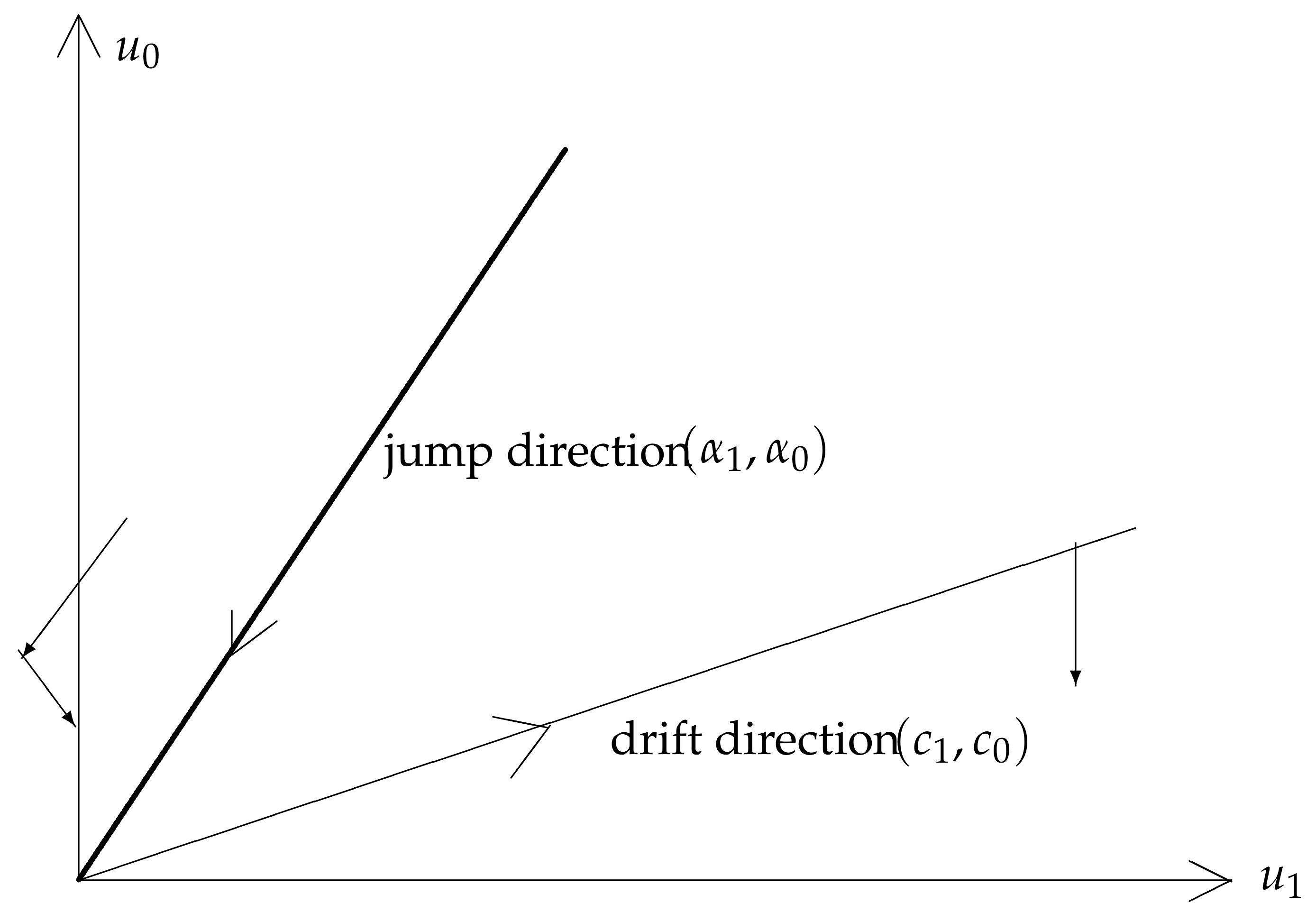
Lemma 1.

Under the cheap reinsurance condition (14), the lower cone

$$\mathcal{C}:=\{0\le u_0\le u_1\frac{{\alpha }_0}{{\alpha }_1}\}$$

contains $c=(c_1,c_0)$, and is thus invariant with respect to the flow, i.e., that starting with initial capital $(u_1,u_0)\in \mathcal{C}$, the process $(X_1,X_0)$ will stay there.

Remark 7.

The boundary $u_0=u_1\frac{{\alpha }_0}{{\alpha }_1}$ will be called “claims line”. The invariance of the lower cone follows from the fact that when claims arrive, the flow is parallel to the claims line and hence cannot cross it. Also, the drift vector points away from the claims line since the angle of the vector $\mathit{\alpha }=({\alpha }_1,{\alpha }_0)$ with the $u_1$ axis is bigger than that of $\mathit{c}=(c_1,c_0)$, and so in the absence of claims the distance to the claims line is increased.

Finally, the only exit possible from the lower cone $\mathcal{C}$ is when ruin happens for the CB/reinsurer $X_0$, see Figure 1, and the ruin probability in this cone is a classic one-dimensional ultimate ruin probability

$$\mathrm{\Psi }(u_1,u_0)=\mathrm{\Psi }({\alpha }_1\frac{u_0}{{\alpha }_0},u_0):={\mathrm{\Psi }}_0(u_0),\forall u_0$$

(see, for example, Albrecher and Asmussen (2010); Rolski et al. (2009)).

For a different application of invariant cones in a multi-dimensional setting, see Section 6.

Since exit from the cone $\mathcal{C}$ is possible only through the boundary $u_0=0$, the Laplace transform corresponding to this boundary may be computed from the one dimensional ruin problem for $X_0$. Determining the last remaining unknown in the Wiener-Hopf type equation is then possible in principle, by the same “cancelation of singularity by annihilating the numerator” technique used to prove the Pollaczek-Khinchine formula.

Showing that a singularity (curve) is indeed removable is naturally more difficult in two dimensions. We have been unable to establish this for our setup, and so we proceed by conjecturing it, leaving this as future work. Note that in a queueing paper with similar setup Badila et al. (2014), an essentially equivalent statement has been established rigorously.

We now obtain the transforms of the survival and ruin probabilities, assuming that the singularity cancelation could be justified. Observe that the survival and ruin probabilities coincide with those of the scaled process $(X_1/{\alpha }_1,X_0/{\alpha }_0)$. Therefore, we may assume w.l.o.g. for this result that ${\alpha }_0={\alpha }_1=1$. Assume the invariance condition (14) and the positive loading condition $r_0:=\frac{{\lambda }_c{m}_c+{\lambda }_0{m}_0}{c_0}<1,$ where $m_c={\int }_0^{\infty }y{f}_c(y)dy$ and $m_0={\int }_0^{\infty }y{f}_0(y)dy$. Then, by invariance and the Pollaczek-Khinchine formula (see (Albrecher and Asmussen 2010, p. 77))

$$\overline{\mathrm{\Psi }}(u_1,0)={\overline{\mathrm{\Psi }}}_0(0)=1-r_0,$$

and (13) reduces to a Riemann-Hilbert equation with two unknowns

$$\begin{array}{c}\hfill (\mathcal{L}\overline{\mathrm{\Psi }})(s_1,s_0)=\frac{c_1{\int }_0^{\infty }\overline{\mathrm{\Psi }}(0,u_0)e^{-s_0{u}_0}d{u}_0+c_0\frac{1-r_0}{s_1}}{\kappa (s_1,s_0)},\end{array}$$

(15)

where $\kappa (s_1,s_0)=c_1{s}_1+c_0{s}_0+{\lambda }_c({\widehat{f}}_c(s_1+s_0)-1)+{\lambda }_0({\widehat{f}}_0(s_0)-1).$

Proposition 1.

Let ${\alpha }_1={\alpha }_0=1$. If the invariance condition (14) and the positive loading condition hold, then the Laplace transform of the ultimate survival probability (15) is given explicitly by:

$$(\mathcal{L}\overline{\mathrm{\Psi }})(s_1,s_0)=c_0(1-r_0)\frac{\frac{1}{s_1}-\frac{1}{{\tilde{s}}_1}}{\kappa (s_1,s_0)},$$

(16)

where ${\tilde{s}}_1={\tilde{s}}_1(s_0)$ is defined in (19).

Proof. 

The denominator of (15) may be written as

$$\kappa (s_1,s_0)={\kappa }_1(s_1+s_0)-\eta (s_0),$$

where for ease of notation we put

$$\begin{array}{cc}\hfill {\kappa }_1(s)& :=c_{1}s+{\lambda }_c({\widehat{f}}_c(s)-1),\hfill \end{array}$$

(17)

$$\begin{array}{cc}\hfill \eta (s)& :=(c_1-c_0)s+{\lambda }_0(1-{\widehat{f}}_0(s)).\hfill \end{array}$$

(18)

Let us look for the nonnegative root of ${\kappa }_1(s_1+s_0)=\eta (s_0)$, i.e., select the root

$$\begin{array}{c}\hfill s_1={\mathrm{\Phi }}_1(\eta (s_0))-s_0:={\tilde{s}}_1(s_0),\end{array}$$

(19)

where we denoted by ${\mathrm{\Phi }}_1(\delta )$ the unique non-negative root of the equation ${\kappa }_1(s)=\delta$, and define the curve

$$\mathrm{\Gamma }=\{(s_1,s_0)|s_0>0,s_1+s_0={\mathrm{\Phi }}_1(\eta (s_0))\}.$$

Now if $\mathrm{\Gamma }$ is a curve of removable singularities, it must also annihilate the numerator, and we conclude that along this curve it holds that

$$\begin{array}{c}{c}_1{\int }_0^{\infty }\overline{\mathrm{\Psi }}(0,u_0)e^{-s_0{u}_0}d{u}_0=\frac{c_0(1-r_0)}{-{\tilde{s}}_1},\end{array}$$

(20)

and (16) holds. ☐

Remark 8.

If ${\lambda }_0=0,c_1=c_0$, then $\eta (s)=0,{\tilde{s}}_1=-s_0,\tau (u_0,u_1)={\tau }_0(u_0\wedge u_1)$, and (16) reduces to $(\mathcal{L}\overline{\mathrm{\Psi }})(s_1,s_0)={\widehat{\overline{\mathrm{\Psi }}}}_0(s_0+s_1)(\frac{1}{s_1}+\frac{1}{s_0}),$ a result which can be easily checked.

We consider now the Laplace transform (8) with $\delta >0,$ assuming for simplicity that ${\alpha }_1={\alpha }_0=1$. The corresponding result is:

Proposition 2.

When ${\alpha }_1={\alpha }_0=1,c_0<c_1$, and the positive loading condition holds, it follows that

$$\mathcal{L}{\varphi }_{\delta }(s_1,s_0)=\frac{1}{s_1{s}_0}-\left(\frac{\delta }{s_0}-\frac{\delta }{{\mathrm{\Phi }}_0(\delta )}\right)\frac{\left(\frac{1}{{\tilde{s}}_1}-\frac{1}{s_1}\right)}{\kappa (s_1,s_0)-\delta }.$$

(21)

Proof. 

First, define ${\kappa }_0(s):=c_{0}s+{\lambda }_c({\widehat{f}}_c(s)-1)+{\lambda }_0({\widehat{f}}_0(s)-1)$ and ${\mathrm{\Phi }}_0(\delta )$, which is the right inverse of ${\kappa }_0$ at $\delta$. The invariance of the lower cone $\{u_0\le u_1\}$ implies

$$\begin{array}{ccc}\hfill \forall u_1,{\varphi }_{\delta }(u_1,0)& =& {\varphi }_{\delta }(0,0)=1-\frac{\delta /{\mathrm{\Phi }}_0(\delta )}{c_0}.\hfill \end{array}$$

Also, (11) becomes

$$\mathcal{L}{\varphi }_{\delta }(s_1,s_0)=\frac{c_1{\int }_0^{\infty }{e}^{-s_0{u}_0}{\varphi }_{\delta }(0,u_0)d{u}_0+\frac{c_0}{s_1}{\varphi }_{\delta }(0,0)-\frac{c_0{s}_0+c_1{s}_1-\delta }{s_1{s}_0}}{\kappa (s_1,s_0)-\delta }+\frac{1}{s_1{s}_0}.$$

(22)

Next, the denominator singularity $\kappa (s_1,s_0)-\delta ={\kappa }_1(s_1+s_0)-(\eta (s_0)+\delta )$ becomes

$$\kappa (s_1,s_0)-\delta =0\iff s_1={\mathrm{\Phi }}_1(\eta (s_0)+\delta )-s_0:={\tilde{s}}_1(s_0),$$

and the curve of presumed removable singularities is

$${\mathrm{\Gamma }}_{\delta }=\{(s_1,s_0)|s_0>0,s_1+s_0={\mathrm{\Phi }}_1(\eta (s_0)+\delta )\}.$$

If ${\tilde{s}}_1(s_0)$ annihilates the numerator as well, we must have

$$\begin{array}{c}{c}_1{\int }_0^{\infty }{e}^{-s_0{u}_0}{\varphi }_{\delta }(0,u_0)d{u}_0=\frac{c_1}{s_0}+\frac{c_0(1-{\varphi }_{\delta }(0,0))}{{\tilde{s}}_1}-\frac{\delta }{{\tilde{s}}_1{s}_0}=\frac{c_1}{s_0}+\frac{\delta /{\mathrm{\Phi }}_0(\delta )}{{\tilde{s}}_1}-\frac{\delta }{{\tilde{s}}_1{s}_0}.\end{array}$$

Plugging the above formula back into the numerator in (22) we get

$$\mathcal{L}{\varphi }_{\delta }(s_1,s_0)=\frac{1}{s_1{s}_0}-\frac{H(s_1,s_0,\delta )}{\kappa (s_1,s_0)-\delta },$$

(23)

where

$$H(s_1,s_0,\delta )=\left(\frac{\delta }{s_0}-\frac{\delta }{{\mathrm{\Phi }}_0(\delta )}\right)\left(\frac{1}{{\tilde{s}}_1}-\frac{1}{s_1}\right).$$

(24)

 ☐

Remark 9.

As $\delta \to 0$, $\frac{\delta }{{\mathrm{\Phi }}_0(\delta )}\to c_0(1-r_0)$ and so (21) becomes

$$\begin{array}{c}\hfill \mathcal{L}\mathrm{\Psi }(s_1,s_0)=\frac{1}{s_0{s}_1}-\frac{c_0(1-r_0)\left(\frac{1}{s_1}-\frac{1}{{\tilde{s}}_1}\right)}{\kappa (s_1,s_0)},\end{array}$$

(25)

which agrees with (16).

Remark 10.

In the particular case ${\lambda }_0=0$, the result may also be obtained by a probabilistic approach (Avram et al. 2008b, p. 23) and use of Suprun’s resolvent formula Suprun (1976); even in this case, the connection between the Formula (16) and the probabilistic interpretation is not straightforward.

5. A Two-Dimensional CB with Proportional Reinsurance and Crisis Bailouts

In this section we introduce bailouts which were not considered in the previous section. We will assume for simplicity that ${\alpha }_1={\alpha }_0=1$, w.l.o.g. (by considering the processes $X_i/{\alpha }_i,i=1,0$, which have the same ruin time as $X_i,i=1,0$). Thus, the model reduces to

$$\begin{array}{c}{X}_1(t):=u_1+c_{1}t-C(t)+Z(t),\hfill \\ X_0(t):=u_0+c_{0}t-C(t)-C_0(t)-kZ(t),k\ge 0.\hfill \end{array}$$

Note that due to the different scalings for $X_i$, we may not assume anymore that $k>1$.

The IDE Equation (9) becomes now

$$\begin{array}{c}({\lambda }_c+{\lambda }_0+\delta ){\varphi }_{\delta }(u_1,u_0)=c_1\frac{\partial }{\partial u_1}{\varphi }_{\delta }(u_1,u_0)+c_0\frac{\partial }{\partial u_0}{\varphi }_{\delta }(u_1,u_0)\hfill \\ +{\lambda }_0{\int }_0^{u_0}{\varphi }_{\delta }(u_1,u_0-x)f_0(x)dx+{\lambda }_0{\overline{F}}_0(u_0)\hfill \\ +{\lambda }_c{\int }_0^{u_1\wedge u_0}{\varphi }_{\delta }(u_1-x,u_0-x)f_c(x)dx+{\lambda }_c{\overline{F}}_c(u_0){\mathbf{1}}_{u_0\le u_1}\hfill \\ +{\lambda }_c{\mathbf{1}}_{u_0>u_1}\left({\int }_{u_1}^{\frac{k{u}_1+u_0}{k+1}}{\varphi }_{\delta }(0,u_0+k{u}_1-(k+1)x)f_c(x)dx+{\overline{F}}_c\left(\frac{k{u}_1+u_0}{k+1}\right)\right).\hfill \end{array}$$

(26)

Remark 11.

The first five terms coincide with those in (9), but the sixth term there splits now into three new terms. The new sixth term corresponds to common ruin of both companies, starting from the cone $u_1>u_0$. The last two terms correspond to a possible jump crossing the boundary $u_1=0$ from the cone $u_1\le u_0$, which is possible if the ruinous claim $C_i\in [x,x+dx],x>u_1$. If furthermore $x>\frac{k{u}_1+u_0}{k+1}$, we have final ruin, yielding the last term. In the opposite case, $X_0$ can cover the bailout, resulting in reflection from the new starting point $\left(0,\frac{k{u}_1+u_0}{k+1}\right)$.

Thus, the Laplace transform of (26) is

$$\begin{array}{c}(\kappa (s_1,s_0)-\delta )\mathcal{L}{\varphi }_{\delta }(s_1,s_0)=c_1{\widehat{\varphi }}_{\delta }(0,s_0)+c_0{\widehat{\varphi }}_{\delta }(s_1,0)-{\lambda }_0\frac{1-{\widehat{f}}_0(s_0)}{s_1{s}_0}-{\lambda }_c(A_0+A_1+A_2),\hfill \end{array}$$

where $A_i,i\in \{0,1,2\}$ are the Laplace transforms of the last three terms.

The sixth transform is straightforward, being:

$$\begin{array}{c}{A}_0=\frac{1-{\widehat{f}}_c(s_1+s_0)}{s_1(s_1+s_0)}.\end{array}$$

We turn now to the last two terms

$$\begin{array}{cc}\hfill A_1& =\int {\int }_{u_0>u_1}{e}^{-s_1{u}_1-s_0{u}_0}{\int }_{u_1}^{\frac{k{u}_1+u_0}{k+1}}{\varphi }_{\delta }(0,u_0+k{u}_1-(k+1)x)f_c(x)dxd{u}_{0}d{u}_1\hfill \\ & ={\int }_0^{\infty }{f}_c(x){\int }_0^x{e}^{-s_1{u}_1}{\int }_{(k+1)x-k{u}_1}^{\infty }{e}^{-s_0{u}_0}{\varphi }_{\delta }(0,u_0+k{u}_1-(k+1)x)d{u}_{0}d{u}_{1}dx\hfill \\ & ={\int }_0^{\infty }{f}_c(x){\int }_0^x{e}^{-s_1{u}_1}{\int }_0^{\infty }{e}^{-s_0(y-k{u}_1+(k+1)x)}{\varphi }_{\delta }(0,y)dyd{u}_{1}dx\hfill \\ & ={\int }_0^{\infty }{f}_c(x){\int }_0^x{e}^{-s_1{u}_1+k{s}_0{u}_1-(k+1)s_{0}x}{\widehat{\varphi }}_{\delta }(0,s_0)d{u}_{1}dx\hfill \\ & ={\widehat{\varphi }}_{\delta }(0,s_0){\int }_0^{\infty }{f}_c(x)e^{-(k+1)x{s}_0}\left(\frac{e^{x(k{s}_0-s_1)}-1}{k{s}_0-s_1}\right)dx\hfill \\ & =\frac{{\widehat{\varphi }}_{\delta }(0,s_0)}{k{s}_0-s_1}\left({\widehat{f}}_c(s_0+s_1)-{\widehat{f}}_c((k+1)s_0)\right)\hfill \end{array}$$

and

$$\begin{array}{cc}\hfill A_2& =\int {\int }_{u_0>u_1}{e}^{-s_1{u}_1-s_0{u}_0}{\overline{F}}_c\left(\frac{k{u}_1+u_0}{k+1}\right)d{u}_{0}d{u}_1\hfill \\ & ={\int }_0^{\infty }{\int }_{u_1}^{\infty }{e}^{-s_1{u}_1-s_0{u}_0}{\int }_{\frac{k{u}_1+u_0}{k+1}}^{\infty }{f}_c(x)dxd{u}_{0}d{u}_1\hfill \\ & ={\int }_0^{\infty }{\int }_{u_1}^{\infty }{\int }_{u_1}^{(k+1)x-k{u}_1}{e}^{-s_0{u}_0}d{u}_0{f}_c(x)e^{-s_1{u}_1}dxd{u}_1\hfill \\ & =\frac{1}{s_0}{\int }_0^{\infty }{\int }_{u_1}^{\infty }(e^{-s_0{u}_1}-e^{-s_0((k+1)x-k{u}_1)})f_c(x)e^{-s_1{u}_1}dxd{u}_1\hfill \\ & =\frac{1}{s_0}{\int }_0^{\infty }{\int }_0^x(e^{-(s_0+s_1)u_1}-e^{-(k+1)x{s}_0+(k{s}_0-s_1)u_1})d{u}_1{f}_c(x)dx\hfill \\ & =\frac{1}{s_0}{\int }_0^{\infty }\left(\frac{1-e^{-(s_0+s_1)x}}{s_0+s_1}-e^{-(k+1)x{s}_0}\frac{e^{(k{s}_0-s_1)x}-1}{k{s}_0-s_1}\right)f_c(x)dx\hfill \\ & =\frac{1}{s_0}\left(\frac{1-{\widehat{f}}_c(s_0+s_1)}{s_0+s_1}+\frac{{\widehat{f}}_c((k+1)s_0)-{\widehat{f}}_c(s_0+s_1)}{k{s}_0-s_1}\right).\hfill \end{array}$$

Therefore we obtain the following theorem:

Theorem 3.

When ${\alpha }_0={\alpha }_1=1$, the Laplace transform of ${\varphi }_{\delta }(u_1,u_0)$ satisfies the Riemann-Hilbert equation with three unknowns

$$\begin{array}{cc}\hfill (\kappa (s_1,s_0)-\delta )\mathcal{L}{\varphi }_{\delta }(s_1,s_0)& =c_1{\widehat{\varphi }}_{\delta }(0,s_0)+c_0\frac{{\varphi }_{\delta }(0,0)}{s_1}+{\lambda }_0\frac{{\widehat{f}}_0(s_0)-1}{s_1{s}_0}\hfill \\ & +{\lambda }_c\left[\frac{{\widehat{f}}_c(s_0+s_1)-1}{s_1{s}_0}-\frac{({\widehat{f}}_c(s_0+s_1)-{\widehat{f}}_c((k+1)s_0))({\widehat{\varphi }}_{\delta }(0,s_0)-1/s_0)}{k{s}_0-s_1}\right]\hfill \\ & =c_1{\widehat{\varphi }}_{\delta }(0,s_0)+c_0\frac{{\varphi }_{\delta }(0,0)}{s_1}+\frac{\kappa (s_1,s_0)-c_0{s}_0-c_1{s}_1}{s_1{s}_0}\hfill \\ & -{\lambda }_c\frac{({\widehat{f}}_c(s_0+s_1)-{\widehat{f}}_c((k+1)s_0))({\widehat{\varphi }}_{\delta }(0,s_0)-1/s_0)}{k{s}_0-s_1}.\hfill \end{array}$$

Remark 12.

When $c_0\le c_1$, an explicit expression for the Laplace transform may be obtained, just as in the previous section (modulo establishing the fact that the singularity from the previous section is removable).

6. Valuation of Risk Networks by Optimal Dividends

6.1. Individual Valuation of Financial Companies

Evaluating financial companies is a very important problem, and a natural approach, going back to De Finetti (1957) and Miller and Modigliani (1961) is to use the optimal expected discounted cumulative dividends/optimal consumption until ruin—see Leobacher et al. (2014) for further references on this venerable approach.

Definition 2.

Let

$$\tilde{X}(t)=X(t)-R(t)$$

denote a process modified by “consumption/dividends”. For $b>0$, a dividend policy ${\pi }_b$ with barrier b consists in taking dividends $dR(t)={(\tilde{X}(t)-b)}^{+}$ up to ruin. We will write the expectation operator ${\mathbb{E}}_x^{b]}$ to indicate this policy and the initial capital x. One says that under ${\mathbb{E}}_x^{b]}$, $\tilde{X}$ follows the dynamics of the process X reflected at b. The ruin time will be denoted by $\tau ={\tau }_0^{-}$.

For spectrally negative Lévy models, all first passage results may be expressed in terms of the W scale function Bertoin (1998); Kyprianou (2014); Suprun (1976). In particular, the formula for the expected discounted cumulative dividends until ruin, when restricting to barrier strategies ${\pi }_b$ has a simple expression:

$$V_{\delta }(x,b)={\mathbb{E}}_x^{|0,b]}\left[{\int }_{[0,{\tau }_0^{-}]}{e}^{-\delta s}dR(s)\right]=\left\{\begin{array}{cc}\frac{W_{\delta }(x)}{W_{\delta }^{\prime }(b)},\hfill & x\le b,\hfill \\ x-b+\frac{W_{\delta }(b)}{W_{\delta }^{\prime }(b)},\hfill & x>b,\hfill \end{array}\right.$$

(27)

where ${\mathbb{E}}^{|0,b]}$ denotes the law of the process reflected from above at b, and absorbed at 0 and below.

6.2. Evaluating a Conglomerate of Companies by Claims Line Dividend Policies

Turning now to several dimensions, the de Finetti objective becomes

$$\begin{array}{c}\hfill {\mathcal{I}}^F(\mathit{u}):=\underset{\pi =(R_0,R_1,\dots ,R_I)}{sup}{E}_{\mathit{u}}{\int }_0^{\tau }{e}^{-qt}\left(\sum _{i=0}^{I}d{R}_i(t)\right),\end{array}$$

(28)

where $R_i$ are the cumulative dividends of the i-th company, and $\tau ={\tau }_{\mathrm{or}}$ is the ruin/liquidation time. In this section, we propose a certain collaborative, multi-dimensional dividends policy, which, remarkably, was found to be optimal in Azcue et al. (2016), if the retention levels are small enough, and which tries to guide the conglomerate along a certain line through the origin. In particular, under this policy ${\tau }_{\mathrm{or}}={\tau }_{\mathrm{all}}$, and the time to ruin is maximized, intuitively. Note that since all companies become bankrupt simultaneously, there is no possibility of bailouts. Generalizing Lemma 1 to several dimensions, we find:

Lemma 2.

If the “cheap reinsurance” condition

$$\begin{array}{c}\hfill c_0\le c_i\frac{{\overline{\alpha }}_i}{{\alpha }_i},i=1,\cdots ,I\end{array}$$

(29)

is satisfied, then the stochastic flow leaves invariant the cone

$$\mathcal{C}:=\{0\le u_0\le u_i\frac{{\overline{\alpha }}_i}{{\alpha }_i},{\overline{\alpha }}_i=1-{\alpha }_i,i=1,\cdots ,I\}.$$

The hero of the story is again the boundary edge

$$\begin{array}{c}{u}_1\frac{1-{\alpha }_1}{{\alpha }_1}=\dots =u_i\frac{1-{\alpha }_i}{{\alpha }_i}=u_0,i=1,\cdots ,I,\end{array}$$

(30)

which is also called the “claims line”. Just as in Lemma 1, it is easy to check that exit from the cone $\mathcal{C}$ cannot happen in the absence of claims, since the process gets further from the claims line and cannot reach the planes which define it. In conclusion, the only possible exit is through the boundary $u_0=0$.

Remark 13.

The claims line plays a prominent role in two recent papers, Bäuerle and Blatter (2011)3 and Azcue et al. (2016), who studied the optimal dividends problem. In the cheap reinsurance two-dimensional case $c_1\frac{1-{\alpha }_1}{{\alpha }_1}\ge c_0,$ Azcue et al. (2016) showed that:

• Starting from the claims line, the optimal policy is to stay on this line by cashing the excess income of the subsidiary as dividends.
• Starting from points away from the claims line, in the cheap reinsurance case, the optimal policy is to reach the claims line by one lump sum payment4.

These findings prompt us to introduce a heuristic “claims line” dividend policy for cheap reinsurance networks, under which the network follows this line in the absence of claims, by subsidiaries cashing part of their premia as dividends. Thus, dividends of rate $c_i-c_0\frac{{\alpha }_i}{{\overline{\alpha }}_i}\ge 0,i=1,\dots ,I$ are continuously paid. Subsequently, whenever a subsidiary i drops by ${\alpha }_{i}C$ due to a claim C, all the other subsidiaries j must also reduce their reserves by a lump sum dividend of $C{\overline{\alpha }}_i\frac{{\alpha }_j}{{\overline{\alpha }}_j}$, bringing back the process on the claims line. Note that no adjustment is required from the CB, since the proportional reinsurance preserves the constraint $u_i\frac{1-{\alpha }_i}{{\alpha }_i}=u_0$. Finally, when a dedicated claim C of the CB arrives, all the subsidiaries j must reduce their reserves by a lump sum dividend of $C\frac{{\alpha }_j}{{\overline{\alpha }}_j}$5.

Remark 14.

By restricting to claim line strategies, the problem of evaluating a network is greatly simplified. The subsidiary processes reduce to linear functions ${\tilde{X}}_i(t)=\frac{{\alpha }_i}{1-{\alpha }_i}{X}_0(t)$ of the CB process, and the expected dividends decompose as a sum of one-dimensional quantities, as seen in the example below and in Lemma 3.

Example 5.

With one subsidiary, under the claims line policy $\pi =(R_0,\tau )$ associated to an admissible CB dividends process $R_0(t)$, and a stopping time τ, the de Finetti value function is:

$$\begin{array}{cc}\hfill V_{\pi }^F(x)& ={\mathbb{E}}_x\left[{\int }_0^{\tau }{e}^{-qt}\left(d{R}_0(t)+(c_1-c_0\frac{{\alpha }_1}{{\overline{\alpha }}_1})dt\right)+\frac{{\alpha }_1}{{\overline{\alpha }}_1}\sum _{k=1}^{N_{{\lambda }_0}(\tau )}{e}^{-q{T}_{k,0}}{C}_{k,0}\right]\hfill \\ & ={\mathbb{E}}_x\left[{\int }_0^{\tau }{e}^{-qt}\left(d{R}_0(t)-\frac{{\alpha }_1}{{\overline{\alpha }}_1}d{X}_0(t)+d{X}_1(t)\right)\right],\hfill \end{array}$$

where $C_{k,0}$ and $T_{k,0}$ denote the CB dedicated claims and their arrival times, respectively.

Lemma 3.

For a general CB network, and a fixed admissible dividends process $R_0(t)$, the de Finetti value function for the equilibrium policy associated to $\pi =(R_0,\tau )$ is:

$$V_{\pi }^F(x)={\mathbb{E}}_x\left[{\int }_0^{\tau }{e}^{-qt}\left[d{R}_0(t)+\sum _{i=1}^{I}d{X}_i(t)-\gamma d{X}_0(t)\right]\right],$$

where

$$\gamma =\sum _{i=1}^I\frac{{\alpha }_i}{{\overline{\alpha }}_i}.$$

Proof. 

With I subsidiaries, the de Finetti value function is:

$$\begin{array}{cc}\hfill V_{\pi }^F(x)& ={\mathbb{E}}_x\left[{\int }_0^{\tau }{e}^{-qt}\left(d{R}_0(t)+\sum _{i=1}^I(c_i-c_0\frac{{\alpha }_i}{{\overline{\alpha }}_i})dt\right)+\gamma \sum _{k=1}^{N_{{\lambda }_0}(\tau )}{e}^{-q{T}_{k,0}}{C}_{k,0}+\sum _{i=1}^I\left(\gamma {\overline{\alpha }}_i-{\alpha }_i\right)\sum _{k=1}^{N_{{\lambda }_i}(\tau )}{e}^{-q{T}_{k,i}}{C}_{k,i}\right]\hfill \\ & ={\mathbb{E}}_x\left[{\int }_0^{\tau }{e}^{-qt}\left[d{R}_0(t)+\sum _{i=1}^{I}d{X}_i(t)-\gamma d{X}_0(t)\right]\right],\hfill \end{array}$$

where $C_{k,i}$ and $T_{k,i}$ denote the claims of the i-th subsidiary and their arrival times, respectively. ☐

Optimizing dividends using our heuristic policy may thus be achieved by solving three one-dimensional problems. The first term is already known (see Equation (27)), whereas the second and third terms ${\mathbb{E}}_x{\int }_0^{\tau }{e}^{-qt}d{X}_i(t)$ and ${\mathbb{E}}_x{\int }_0^{\tau }{e}^{-qt}d{X}_0(t)$ can be handled integrating by parts and applying classic one-dimensional methods (see for example Avram et al. (2017); Kyprianou (2014), for a textbook and review, respectively). This will be pursued in a future paper.

7. Conclusions

In this paper, we have introduced a risk network model involving a new type of cooperation between a central branch and its subsidiaries, which involves both bail-out interventions during “critical moments”, and continuous reinsurance of each claim. In the particular case of large enough proportional reinsurance, explicit solutions via Laplace transforms are possible, whereas they would be impossible without.

We believe that more important than the rather particular mathematical results obtained are the questions implicitly raised.

• Can the performance of a risk network be improved by using stop-loss reinsurance, or proportional reinsurance, or a combination of the two, or reinsurance strategies recently studied by Tan et al. (2018)?
• Our model considers intervention of the central branch at ruin times; however, other intervention times such as draw-down/regret times and Parisian ruin times may result in better network performance.

These questions are left for future work and will require intensive numerical investigation. Finally, note that while we focused on a model with one reinsurer, realistic applications will require treating multiple reinsurers—see for example Boonen et al. (2016, 2018); Chi and Meng (2014).

References

- Asmussen, Søren, and Hansjörg Albrecher. 2010. Ruin Probabilities. Singapore: World Scientific, vol. 14. [Google Scholar]
- Albrecher, Hansjörg, Jevgenijs Ivanovs, and Xiaowen Zhou. 2016. Exit identities for Lévy processes observed at Poisson arrival times. Bernoulli 22: 1364–82. [Google Scholar] [CrossRef]
- Avram, Florin, and Andreea Minca. 2015. Steps towards a management toolkit for central branch risk networks, using rational approximations and matrix scale functions. In Modern Trends in Controlled Stochastic Processes: Theory and Applications. Edited by Alexey B. Piunovskyi. Luniver Press. [Google Scholar]
- Avram, Florin, and Andreea Minca. 2017. On the central management of risk networks. Advances in Applied Probability 49: 221–37. [Google Scholar] [CrossRef]
- Avram, Florin, and Xiaowen Zhou. 2016. On fluctuation theory for spectrally negative Lévy processes with Parisian reflection below, and applications. Theory of Probability and Mathematical Statistics 95: 14–36. [Google Scholar] [CrossRef]
- Avram, Florin, Martijn R. Pistorius, and Zbigniew Palmowski. 2006. A two-dimensional ruin problem on the positive quadrant, with exponential claims: Feynman-Kac formula, Laplace transform and its inversion. Paper presented at Ninth International Conference Zaragoza-Pau on Applied Mathematics and Statistics, Jaca, Spain, September 19–21. [Google Scholar]
- Avram, Florin, Zbigniew Palmowski, and Martijn R. Pistorius. 2007. On the optimal dividend problem for a spectrally negative Lévy process. The Annals of Applied Probability 17: 156–80. [Google Scholar] [CrossRef]
- Avram, Florin, Zbigniew Palmowski, and Martijn R. Pistorius. 2008a. Exit problem of a two-dimensional risk process from the quadrant: Exact and asymptotic results. The Annals of Applied Probability 18: 2421–49. [Google Scholar] [CrossRef]
- Avram, Florin, Zbigniew Palmowski, and Martijn R. Pistorius. 2008b. A two-dimensional ruin problem on the positive quadrant. Insurance: Mathematics and Economics 42: 227–34. [Google Scholar] [CrossRef]
- Avram, Florin, Andrei Badescu, Martijn R. Pistorius, and Landy Rabehasaina. 2016. On a class of dependent Sparre Andersen risk models and a bailout application. Insurance: Mathematics and Economics 71: 27–39. [Google Scholar] [CrossRef]
- Avram, Florin, Danijel Grahovac, and Ceren Vardar-Acar. 2017. The W,Z scale functions kit for first passage problems of spectrally negative Lévy processes, and applications to the optimization of dividends. arXiv, arXiv:1706.06841. [Google Scholar]
- Avram, Florin, José-Luis Pérez, and Kazutoshi Yamazaki. 2018. Spectrally negative Lévy processes with Parisian reflection below and classical reflection above. Stochastic Processes and Applications 128: 255–90. [Google Scholar] [CrossRef]
- Avram, Florin. 2017. Approximating central branch networks with one subsidiary via spectrally negative Markov additive processes. Work in Progress. Forthcoming. [Google Scholar]
- Azcue, Pablo, Nora Muler, and Zbigniew Palmowski. 2016. Optimal dividend payments for a two-dimensional insurance risk process. arXiv, arXiv:1603.07019. [Google Scholar]
- Badescu, Andrei L., Eric CK Cheung, and Landy Rabehasaina. 2011. A two-dimensional risk model with proportional reinsurance. Journal of Applied Probability 48: 749–65. [Google Scholar] [CrossRef]
- Badila, Serban E., Onno Boxma, Jacques Resing, and Erik Winands. 2014. Queues and risk models with simultaneous arrivals. Advances in Applied Probability 46: 812–31. [Google Scholar] [CrossRef]
- Bertoin, Jean. 1998. Lévy Processes. Cambridge: Cambridge University Press, vol. 121. [Google Scholar]
- Boonen, Tim J., Ken Seng Tan, and Sheng Chao Zhuang. 2016. The role of a representative reinsurer in optimal reinsurance. Insurance: Mathematics and Economics 70: 196–204. [Google Scholar] [CrossRef]
- Boonen, Tim J., Ken Seng Tan, and Sheng Chao Zhuang. 2018. Optimal Reinsurance with Multiple Reinsurers: Competitive Pricing and Coalition Stability. Available online: https://papers.ssrn.com/sol3/papers.cfm?abstract_id=3143224 (accessed on 11 April 2018).
- Boxma, Onno, and Jevgenijs Ivanovs. 2013. Two coupled Lévy queues with independent input. Stochastic Systems 3: 574–90. [Google Scholar] [CrossRef]
- Boxma, Onno, Esther Frostig, David Perry, and Rami Yosef. 2016. Partial coverage by a rich uncle until ruin: A reinsurance model. Research Report Eurandom 2016: 1. [Google Scholar]
- Boxma, Onno, Esther Frostig, and David Perry. 2017a. A reinsurance risk model with a threshold coverage policy: The Gerber–Shiu penalty function. Journal of Applied Probability 54: 267–85. [Google Scholar] [CrossRef]
- Boxma, Onno, Esther Frostig, David Perry, and Rami Yosef. 2017b. A state dependent reinsurance model. Insurance: Mathematics and Economics 74: 170–81. [Google Scholar] [CrossRef]
- Bäuerle, Nicole, and Anja Blatter. 2011. Optimal control and dependence modeling of insurance portfolios with Lévy dynamics. Insurance: Mathematics and Economics 48: 398–405. [Google Scholar] [CrossRef]
- Cai, Jun, and Haijun Li. 2005. Multivariate risk model of phase type. Insurance: Mathematics and Economics 36: 137–52. [Google Scholar] [CrossRef]
- Chan, Wai-Sum, Hailiang Yang, and Lianzeng Zhang. 2003. Some results on ruin probabilities in a two-dimensional risk model. Insurance: Mathematics and Economics 32: 345–58. [Google Scholar] [CrossRef]
- Chi, Yichun, and Hui Meng. 2014. Optimal reinsurance arrangements in the presence of two reinsurers. Scandinavian Actuarial Journal 2014: 424–38. [Google Scholar] [CrossRef]
- De Finetti, Bruno. 1957. Su un’impostazione alternativa della teoria collettiva del rischio. Paper presented at the Transactions of the XVth International Congress of Actuaries, New York, NY, USA, June 6; pp. 433–43. [Google Scholar]
- Frostig, Esther. 2008. On ruin probability for a risk process perturbed by a Lévy process with no negative jumps. Stochastic Models 24: 288–313. [Google Scholar] [CrossRef]
- Hu, Zechun, and Bin Jiang. 2013. On joint ruin probabilities of a two-dimensional risk model with constant interest rate. Journal of Applied Probability 50: 309–22. [Google Scholar] [CrossRef]
- Hult, Henrik, and Filip Lindskog. 2006. Heavy-Tailed Insurance Portfolios: Buffer Capital and Ruin Probabilities. Technical Report, 1441. Ithaca: School of ORIE Cornell University. [Google Scholar]
- Kabanov, Yuri, and Mher Safarian. 2009. Markets with Transaction Costs: Mathematical Theory. New York: Springer. [Google Scholar]
- Kabanov, Yuri. 1999. Hedging and liquidation under transaction costs in currency markets. Finance and Stochastics 3: 237–48. [Google Scholar] [CrossRef]
- Kriele, Marcus, and Jochen Wolf. 2014. Value-Oriented Risk Management of Insurance Companies. New York: Springer Science & Business Media. [Google Scholar]
- Kyprianou, Andreas E. 2014. Fluctuations of Lévy Processes with Applications: Introductory Lectures. New York: Springer Science & Business Media. [Google Scholar]
- Leobacher, Gunther, Michaela Szölgyenyi, and Stefan Thonhauser. 2014. Bayesian dividend optimization and finite time ruin probabilities. Stochastic Models 30: 216–49. [Google Scholar] [CrossRef]
- Li, Junhai, Zaiming Liu, and Qihe Tang. 2007. On the ruin probabilities of a bidimensional perturbed risk model. Insurance: Mathematics and Economics 41: 185–95. [Google Scholar] [CrossRef]
- Li, Bo, Rong Wu, and Min Song. 2009. A renewal jump-diffusion process with threshold dividend strategy. Journal of Computational and Applied Mathematics 228: 41–55. [Google Scholar] [CrossRef]
- Li, Xiaohu, Jintang Wu, and Jinsen Zhuang. 2015. Asymptotic Multivariate Finite-time Ruin Probability with Statistically Dependent Heavy-tailed Claims. Methodology and Computing in Applied Probability 17: 463–477. [Google Scholar] [CrossRef]
- Liu, Jingchen, and Jae-Kyung Woo. 2014. Asymptotic analysis of risk quantities conditional on ruin for multidimensional heavy-tailed random walks. Insurance: Mathematics and Economics 55: 1–9. [Google Scholar] [CrossRef] [Green Version]
- Loisel, Stephane. 2005. Differentiation of some functionals of risk processes, and optimal reserve allocation. Journal of Applied Probability 42: 379–92. [Google Scholar] [CrossRef]
- Miller, Merton H., and Franco Modigliani. 1961. Dividend policy, growth, and the valuation of shares. The Journal of Business 34: 411–433. [Google Scholar] [CrossRef]
- Rolski, Tomasz, Hanspeter Schmidli, Volker Schmidt, and Jozef L. Teugels. 2009. Stochastic Processes for Insurance and Finance. Hoboken: John Wiley & Sons, vol. 505. [Google Scholar]
- Salah, Zied Ben, and Jose Garrido. 2017. On Fair Reinsurance Premiums; Capital Injections in a Perturbed Risk Model. arXiv, arXiv:1710.11065. [Google Scholar]
- Suprun, V. 1976. Problem of destruction and resolvent of a terminating process with independent increments. Ukrainian Mathematical Journal 28: 39–51. [Google Scholar] [CrossRef]
- Tan, Ken Seng, Pengyu Wei, Wei Wei, and Sheng Chao Zhuang. 2018. Optimal Dynamic Reinsurance Policies Under Mean–CVaR–A Generalized Denneberg’s Absolute Deviation Principle. Available online: https://papers.ssrn.com/sol3/papers.cfm?abstract_id=3138804 (accessed on 11 April 2018).
- Zhang, Zhimin, Hailiang Yang, and Hu Yang. 2013. On a Sparre Andersen risk model perturbed by a spectrally negative Lévy process. Scandinavian Actuarial Journal 2013: 213–39. [Google Scholar] [CrossRef]