Credit Risk Analysis Using Machine and Deep Learning Models †

1
Direction du Numérique, AFD—Agence Française de Développement, Paris 75012, France
2
Laboratory of Excellence for Financial Regulation (LabEx ReFi), Paris 75011, France
3
IPAG Business School, University Paris 1 Pantheon Sorbonne, Ca’Foscari Unversity of Venezia, Venezia 30123, Italy
4
Université Paris 1 Panthéon-Sorbonne, CES, 106 bd de l’Hôpital, Paris 75013, France
5
Capgemini Consulting, Courbevoie 92400, France
6
University College London Computer Science, 66-72 Gower Street, London WC1E 6EA, UK
*
Author to whom correspondence should be addressed.
†
The opinions, ideas and approaches expressed or presented are those of the authors and do not necessarily reflect any past or future Capgemini’s positions. As a result, Capgemini cannot be held responsible for them.
Risks 2018, 6(2), 38; https://doi.org/10.3390/risks6020038
Submission received: 9 February 2018
/
Revised: 3 April 2018
/
Accepted: 9 April 2018
/
Published: 16 April 2018
(This article belongs to the Special Issue Computational Methods for Risk Management in Economics and Finance)
Abstract
:Due to the advanced technology associated with Big Data, data availability and computing power, most banks or lending institutions are renewing their business models. Credit risk predictions, monitoring, model reliability and effective loan processing are key to decision-making and transparency. In this work, we build binary classifiers based on machine and deep learning models on real data in predicting loan default probability. The top 10 important features from these models are selected and then used in the modeling process to test the stability of binary classifiers by comparing their performance on separate data. We observe that the tree-based models are more stable than the models based on multilayer artificial neural networks. This opens several questions relative to the intensive use of deep learning systems in enterprises.
1. Introduction
The use of algorithms raises many ethical questions. Beyond the technical skills required to understand them, algorithms require referrals to the various discussions that occurred in the past years regarding the use of personal data and all the problems related to Big Data, particularly the General Data Protection Regulation (GDPR) directive (GDPR (2016)) arriving 25 May 2018. During the year 2017, a public consultation by the Commission Nationale de L’informatique et des Libertés CNIL (2017), in France, on the use and the development of algorithms was addressed, which led to many conferences and public meetings on artificial intelligence in France. What exactly is the problem? People are afraid of the use of personal data and do not exactly understand the role of the algorithms due to the fear that those algorithms will have decisional power instead of people. These questions and the debates around these ideas are legitimate.
In this paper, we will focus on the algorithms that are used to make these decisions. Algorithms are used in different domains with different objectives. For instance, they are used in enterprises to recruit persons suitable for the profile proposed. Algorithms can simplify the process, make it quicker and more fluid, etc. Nevertheless, algorithms are a set of codes with specific objectives to attain certain objectives. For instance, in the process of recruitment, it can introduce discrimination or a specific profile, and then, “format” the persons working in the enterprise. It is the same in the case of loan provisions, from a bank to an enterprise, where the decision depends on the algorithm used. Thus, it is important to understand these kinds of abuses and to find ways to control the use of the algorithms. Indeed, in this paper, we illustrate the fact that there exist several algorithms that can be used in parallel to answering a question, for instance, to provide a loan to an enterprise. We observe that there exist several strategies to attain our objective of finding the choice of the variables (or features), the criteria and the algorithm that provide an answer to the question.
In this new digital and Big Data era, transparency is necessary; it should be one that does not stand in the way of innovation, but allows for transformation and progress. The terms associated with this field must be ethical, transparent, well known and clear. To contribute to these objectives, some strategic choices are necessary for the training of data experts on the use of machine learning and deep learning algorithms, and the limitations on their usage. This paper attempts to highlight the importance of the choice of algorithms, the choice of the parameters, the selection of relevant variables (features), the role of the evaluation criteria and the importance of humans when it comes to the final decision.
The novelty of this paper lies in addressing some specific questions we encounter when we want to use Big Data and algorithms. We focus mainly on the questions related to the use of the algorithms to solve or attain an objective. The paper Khandani et al. (2010) is the most like ours in applying machine learning models to a large financial dataset with a focus on a single bank. Our paper is differentiated from Khandani et al. (2010) in significant ways. The first is that, unlike Khandani et al. (2010), who focus on the creation of a cardinal measure for consumer credit default and delinquency using a generalized classification and regression trees (CART)-like algorithm, we focus on credit risk scoring where we examine the impact of the choice of different machine learning and deep learning models to identify defaults by enterprises. On the other hand, we do study the stability of these models relative to a choice of subset of variables selected by the models.
Related approaches have been used by Butaru et al. (2016), which investigates consumers delinquency using C4.5 decision trees, logistic regression and random forest with data from six different banks. The work in Galindo and Tamayo (2000) tests CART decision-tree algorithms on mortgage-loan data to detect defaults, and also they compare their results to the k-nearest neighbor (KNN), ANN and probit models. The work in Huang et al. (2004) provides a survey of these models and other related studies.
Although it is unclear how banks decide who to give loans to, the use of classical linear models is well known in the banking sector. Thus, in the present exercise, we use the elastic net approach Zhou and Hastie (2005) as a benchmark, and we compare its fitting and decision rule based on the area under the curve (AUC), as well as root-mean-square error (RMSE) criteria with other non-parametric models classified as machine learning and deep learning in recent literature. We have retained six approaches: a random forest model, a gradient boosting machine and four deep learning models. We specify the models and the choice retained (after optimization procedures) for the parameters of each model. Besides the choice of the model, another question that arises is concerned with the choice of the variables (or features) to decide if an enterprise is eligible for a loan or not. We have used data provided by a European bank (thus, nothing is arbitrary in our further discussion) to analyze the way in which the algorithms used or retained the variables.
This exercise exhibits three key points: the necessity to use (i) several models, (ii) several sets of data (making them change to quantify their impact) and, lastly, (iii) several criteria. We observe that the choices of the features are determinant as are the criteria: they permit one to show the difficulty of getting a unique or “exact” answer and the necessity of analyzing all the results in detail or introducing new information before making any decision. One very important point is the fact that the deep learning model does not necessarily provide very interesting results. Finally, we find that tree-based algorithms have high performances on the binary classification of problems compared to the deep learning models considered in our analysis.
This paper is organized as follows: In Section 2, a unified description of the algorithms that we use is given. Section 3 discusses the criteria used to classify our results, and imbalanced datasets are discussed. The parameters and criteria used for each model are given in Section 4 with the results, and we use them analyze how the algorithms are used to provide a loan to a company. We also analyze in detail the choice of the features retained by each algorithm and their impact on the final results. Section 5 provides the conclusion.
2. A Unified Presentation of Models
The models we use in our application are now presented. We make the presentation as uniform as possible to be able to specify, for each model, the different choices we are confronted with in (i) parameters, (ii) stopping criteria and (iii) activation functions. References are provided for more details.
2.1. Elastic Net
Linear regression is a very well-known approach. It has several extensions; one is the Lasso representation Tibschirani (1996), and another one includes the elastic net approach with a penalty term that is part or Zhou and Hastie (2005).1 In their paper Friedman et al. (2010), describe algorithms for the carrying out of related Lasso models: they propose fast algorithms for fitting generalized linear models with the elastic net penalty. This methodology can be useful for big datasets as soon as the algorithm is built to outperform execution speed. The regression modeling can be linear, logistic or multinomial. The objective is prediction and the minimization of the predictions error, improving both the choice of the model and the estimation procedure.
Denoting Y as the response variable and X the predictors (centered and standardized) and considering a dataset , , the elastic net approach solves the following problem for a given :
where the elastic net penalty is determined by the value of :
Thus,
is the elastic-net penalty term and is a compromise between the ridge regression () and the Lasso penalty (): the constraint for minimization is that for some t. The parameter p is the number of parameters. Historically, this method has been developed when p is very large compared to N. The ridge method is known to shrink the coefficients of the correlated predictors towards each other, borrowing strength from each other. Lasso is indifferent to correlated predictors. Thus, the role of is determinant: in the presence of the correlation, we expect close to one (, for small ). There also exists some link between and . Generally, a grid is considered for as soon as is fixed. A () penalty term could also be considered for prediction.
The algorithm also proposes a way to update the computation, optimizing the number of operations that need to be done. It is possible to associate a weight with each observation, which does not increase the computational cost of the algorithm as long as the weights remain fixed. The previous approach works for several models:
- Linear regression: The response belongs to R. Thus, we use the model (1). In that case, the parameter of interest is , and another set of parameters to be estimated is . The existence of correlation must be considered to verify if the values used for those parameters are efficient or not.
- Logistic regression: The response is binary (0 or 1). In that case, the logistic regression represents the conditional probabilities through a nonlinear function of the predictors where , then we solve:
- Multinomial regression: The response has possibilities. In that case, the conditional probability is2:
For estimation, the parameter must be chosen first, then the simple least squares estimates can be used for linear regression, but a soft threshold is introduced to consider the penalty term, through the decrementing of the parameter using loops. In the case of logistic regression, a least square approach is also considered. In the case of the multinomial regression, constraints are necessary for the use of the regularized maximum likelihood. In any case, the Newton algorithm is implemented.
2.2. Random Forest Modeling
Random forests are a scheme proposed by Breiman (2000); Breiman (2004) to build a predictor ensemble with a set of decision trees that grows in randomly-selected subspaces of data; see Biau (2012); Geurts et al. (2006), and for a review, see Genuer et al. (2008). A random forest is a classifier consisting of a collection of tree-structured classifiers where the are independent identically distributed random variables used to determine how the successive cuts are performed when building the individual trees. The accuracy of a random forest depends on the strength of the individual tree classifiers and the measure of the dependence between them. For each input X, the procedure will be able to predict, with the optimal number of trees, the output value one or zero. A stopping criteria will be used to minimize the error of the prediction.
More precisely, the random trees are constructed in the following way: all nodes of the trees are associated with rectangular cells such that at each step of the construction of the tree, the collection of the cells associated with the leaves of the tree (external nodes) forms a partition of , ). The procedure is repeated many times: (i) at each node, a coordinate of the input is selected with the j-th feature having a probability of being selected; (ii) at each node, once the coordinate is selected, the split is at the midpoint of the chosen side. At each node, randomness is introduced by selecting a small group of input features to split on and choosing to cut the cell along the coordinate.
Each randomized output tree is the average over all the output observations for which the corresponding variables fall in the same cell of the random partition as X. Denoting , the rectangular cell of the random partition containing X, we obtain:
where . We take the expectation of the with respect to the parameter to obtain the estimate of . In practice, the expectation is evaluated by Monte Carlo simulation, that is by generating M (usually large) random trees and taking the average of the individual outcomes. The randomized variables are used to determine how the successive cuts are performed when building the individual trees.
If X has a uniform distribution on , then the response of the model is:
where S is a non-empty subset of d features. With this model, we choose the following parameters: the number of trees and the stopping criteria (called the threshold in the literature) used to choose among the most significant variables. Depending on the context and the selection procedure, the informative probability may obey certain constraints such as positiveness and . The number M of trees can be chosen. It is known that for randomized methods, the behavior of prediction error is a monotonically decreasing function of M; so, in principle, the higher the value of M, the better it is from the accuracy point of view. In practice, in our exercise, we will fit the following non-parametric function on the variables to get the response Y:
where B is the number of trees, and a stopping criteria is used, for which p has to be chosen.
2.3. A Gradient Boosting Machine
We now consider a more global approach for which the previous one can be considered as a special case. Using the previous notations, Y for outputs and X for different N input variables, we estimate a function f mapping X to Y, minimizing the expected value of some specified loss function . This loss function can include squared error , absolute error , for , negative binomial likelihood when , M-regression considering outliers if , if with a transition point and logistic binomial log-likelihood: . A general representation could be:
where the function is a parametric or a non-parametric function of the input X characterized by the parameters .
For estimation purpose, as soon as we work with a finite sample, the parameter optimization is obtained using a greedy stage-wise approach solving:
Thus:
Equations (8) and (9) are called boosting when and are either an exponential loss function or a negative binomial log-likelihood. The function is usually a classification tree. The smoothness constraint defined in (8) can be difficult to minimize and is replaced by a gradient boosting procedure (steepest-descent procedure) detailed in Friedman (2001) or Friedman et al. (2001).
2.4. Deep Learning
Neural networks have been around even longer, since early supervised neural networks were essentially variants of linear regression methods going back at least to the early 1800s. Thus, while learning, networks with numerous non-linear layers date back to at least 1965; also, explicit deep learning research results have been published since at least 1991. The expression “deep learning” was actually coined around 2006, when unsupervised pre-training of deep learning appeared through gradient enhancements and automatic learning rate adjustments during the stochastic gradient descent.
A standard neural network consists of many simple, connected processors called neurons, each producing a sequence of real-valued activations. Input neurons get activated through sensors perceiving the environment; other neurons get activated through weighted connections from previously active neurons. An efficient gradient descent method for teacher-based supervised learning in discrete, differentiable networks of arbitrary depth, called backpropagation, was developed in the 1960s and 1970s, and applied to neural networks in 1981. Deep learning models became practically feasible to some extent through the help of unsupervised learning. The 1990s and 2000s also saw many improvements of purely supervised deep learning. In the new millennium, deep neural networks have finally attracted wide-spread attention, mainly by outperforming alternative machine learning methods such as kernel machines Vapnik (1995); Schölkopf et al. (1998) in numerous important applications. Deep neural networks have become relevant for the more general field of reinforcement learning where there is no supervising teacher.
Deep learning approaches consist of adding multiple layers to a neural network, though these layers can be repeated. Discussing the matter, most deep learning strategies rely on the following four types of architectures: (i) convolutional neural networks, which, in essence, are standard neural networks that have been extended across space using shared weights; (ii) recurrent neural networks, which are standard neural networks that have been extended across time by having edges that feed into the next time step instead of into the next layer in the same time step; (iii) recursive neural networks, which are apparently hierarchical networks where there is no time aspect to the input sequence, but inputs have to be processed hierarchically as in a tree; and finally, (iv) standard deep neural networks, which are a combination of layers of different types without any repetition or particular order. It is this last type that has been implemented in this paper.
In all these approaches, several specific techniques that we do not detail here are used. They concern (i) backpropagation, which is a method to compute the partial derivatives, i.e., the gradient of a function. In this paper, we use the stochastic gradient descent, which is a stochastic approximation of the gradient descent optimization and iterative method for minimizing an objective function that is written as a sum of differentiable functions. Adapting the learning rate for the stochastic gradient descent optimization procedure can increase performance and reduce training time. The simplest and perhaps most used adaptations of learning rate during training are techniques that reduce the learning rate over time. (ii) Regularization in deep learning: This approach consists of randomly dropping units (along with their connections) from the neural network during training. This prevents units from co-adapting too much. During training, dropout has been shown to improve the performance of neural networks on supervised learning tasks in vision, speech recognition, document classification and computational biology, obtaining state-of-the-art results on many benchmark datasets. It has shown no interest in our exercise. (iii) Dimensionality reduction is usually necessary for implementing deep learning strategies. Max pooling can be used for this objective. This was not pertinent in our exercise. For further reading, one can look at Siegelmann and Sontag (1991); Balzer (1985); Deville and Lau (1994); and Hinton and Salakhutdinov (2006). For a complete and recent review, we refer to Schmidhuber (2014); Angelini et al. (2008); Bahrammirzaee (2010); Sirignan et al. (2018).
The neural networks’ behavior or program is determined by a set of real-valued parameters or weights . To represent it in a uniform way, we focus on a single finite episode or epoch of information processing and activation spreading, without learning through weight changes. During an episode, there is a partially causal sequence of real values called events. Each is an input, or the activation of a unit that may directly depend on other through the current neural network. Let the function f encode information and map events to weight indexes. The function f is any nonlinear function. Thus, a classical neural network layer performs a convolution on a given sequence X, outputting another sequence Y, the value of which at time t is as follows:
where are the parameters of the layer trained by backpropagation. In our exercise, along with backpropagation, we have used hierarchical representation learning, weight pattern replication and sub-sampling mechanisms. We make use of the gradient descent method for optimization convergence. The parameters we can choose are the number of layers and the stopping criteria. In the case of an unsupervised deep learning system, regularization functions are added as activation functions. We specify them when we analyze the datasets and the results.
3. The Criteria
There are several performance measures to compare the performance of the models including AUC, Gini, RMSE and Akaike information criterion (AIC); in addition to different metrics like the F-score, the recall and the precision. In this paper, we will mainly present results on the AUC and RMSE criteria, although the results of the other metrics can be made available.
The Gini index was introduced by Gastwirth (1972) and extended by Yitzhaki (1983) and Lerman and Yitzhaki (1984). This index, in essence, permits one to compare several algorithms. It is based on the decision tree methodology and entropy measure. The work in Raileanu and Stoffel (2004) discussed the possibility to compare algorithms using classification systems. From the empirical point of view, this problem has been discussed greatly. It seems that no feature selection rule is consistently superior to another and that Gini can be used to compare the algorithms; nevertheless, we will not use it in the paper, focusing on the ROC curve for which the interpretation in terms of risks is more efficient3.
For each company, we build the ROC curve. An ROC curve is then used to evaluate the quality of the model. The ROC approach can be often associated with the computation of an error from a statistical point of view. If we want to associate the AUC value (coming from the ROC building) to Type I and Type II errors, we need to specify the test we consider and, thus, to determine the hypotheses, the statistics, the level and the power of the test. In our case, the objective is to know if a bank can provide a loan to the enterprise, in the sense that the enterprise will not default. To answer this question, we use several models or algorithms, and the idea is to find the algorithm that permits answering this question with accuracy. The AUC criteria are used to do it; here, we explain why. To analyze, in a robust way, the results obtained with this indicator, we specify the risks associated with it. When a bank provides a loan to an enterprise, it faces two types of errors: (1) to refuse a loan to a company whose probability of default is much lower than the one obtained with the model (Type I error); (2) to agree to provide a loan to a company whose probability of default is much higher than the value obtained with the selected model (Type II error). We want these two errors to be as small as possible. We compute the probability of the corresponding events under the null and the alternative hypotheses. We assume that a bank provides a loan, and the null hypothesis is The company can reimburse the loan, = P[the bank does not provide a loan | the company can reimburse it] = [the bank does not provide a loan]; this is the Type I error; thus, the alternative is The company does not reimburse the loan, and = P[the bank provides a loan | the company cannot pay it back] = [the bank provides a loan]; this is the Type II error.
Considering the dataset, the bank could provide a loan as the probability of default of the target company is sufficiently low (the model outcome has the value of one) or the bank could decide not to provide a loan as the probability of default of the target company is not low enough (the outcome is now zero). These outcomes, one or zero, depend on many variables that we use to compute the risks or . Note that to build the ROC curve, we make varying (it is not fixed as it is in the general context of statistical tests). When we build the ROC, on the x-axis, we represent , also called specificity (in some literature). We want this number close to one4. On the y-axis, we represent , which corresponds to the power of the test, and we want it to be close to one. It is usually referred to as sensitivity5. In practice, when the ROC curve is built, all the codes are done under two kinds of assumptions on the data: the data are independent, and the distributions under the null and the alternative are Gaussian; these assumptions can be far from reality in most cases. From the ROC curve, an AUC is built. The AUC represents the area under the curve. How can we interpret its value? If the curve corresponds to the diagonal, then the AUC is equal to 0.5; we have one chance out of two to make a mistake. If the curve is above the diagonal, the value will be superior to 0.5, and if it attains the horizontal at one, for all , the optimal value of one is obtained. Thus, as soon as the AUC value increases from 0.5–1, it means that we have less and less chance to make a mistake, whatever the value of between zero and one (which means that the Type I error diminishes). It is assumed that the test becomes more and more powerful as the probability for the bank to provide a loan to an enterprise that does not default is very high. Each algorithm provides a value of AUC. To be able to compare the results between the algorithms, we need to verify that we use the same variables to get the outputs one or zero. If that is not the case, the comparison will be difficult and could be biased Seetharaman et al. (2017).
Another question affects the quality of the results: it concerns imbalanced data. The presence of a strong imbalance in the distribution of the response (which is the case for our exercise) creates a bias in the results and weakens the estimation procedure and accuracy of the evaluation of the results. A dataset is imbalanced if the classification categories are not approximately equally represented. Examples of imbalanced datasets have been encountered in many fields, and some references are Mladenic and Grobelnik (1999) or Kubat et al. (1999), among others. Several approaches are used to create balanced datasets, either by over-sampling the minority class and under-sampling the majority class (Kubat and Marvin (1997) or Ling and Li (1998)); diverse forms of over-sampling can be used such as the Synthetic Minority Over-sampling Technique (SMOTE) algorithm developed by Chawla et al. (2002). In this paper, the latter methodology has been implemented, blending under-sampling of the majority class with a special form of over-sampling of the minority class associated with a naive Bayes classifier, improving the re-sampling, modifying the loss ratio and class prior approaches; see also Menardi and Torelli (2011).
The approach that we use, the SMOTE algorithm, proposes an over-sampling approach in which the minority class is over-sampled by creating “synthetic” examples rather than by over-sampling with replacement. The synthetic examples are generated by operating in “feature space” rather than in “data space”. The minority class is over-sampled by taking each minority class sample and introducing synthetic examples along the line segments joining any/all the k minority class neighbors randomly chosen. To generate the synthetic examples, we proceed on the following path: we take the difference between the feature vector under consideration and its nearest neighbor. We multiply this difference by a random number between zero and on and add it to the feature vector under consideration. This causes the selection of a random point along the line segment between two specific features. This approach effectively forces the decision region of the minority class to become more general. The majority class is under-sampled by randomly removing samples from the majority class population until the minority class becomes some specified percentage of the majority class. This forces the learner to experience varying degrees of under-sampling; and at higher degrees of under-sampling, the minority class has a large presence in the training set. In our exercise, the rare events, n, correspond to less than 2% of the whole sample N (n = 1731, and N = 117,019).
4. Data and Models
In this section6, we provide an overview of the data structure and models and then present the results of model performance.
4.1. The Data
The information set contains 117,019 lines, each of them representing either a default or not a default (binary value) of an enterprise when they ask for a loan from a bank. Default and good health are characterized by the same 235 labeled variables that are directly obtained from the companies: financial statements, balance sheets, income statements and cash flows= statements where the values are considered at the lowest level of granularity. In the year 2016/2017, 115,288 lines represented companies in good health and 1731 represented companies in default. Because of the bias created by imbalanced data, in this exercise, we provide only results with balanced training data of the binary classes, following the method recalled in Section 3.
After importing the data, we cleaned the variables and removed features with no pertinent information (same value for all the enterprises; sign with no available entries like ‘NaN’ (Not a Number), for instance) and were left with 181 variables. Then, we split the data into three subsets, considering 80% of the data (60% for the fitting and 20% for the cross-validation), and then 20% of these data was used for test purposes. The validation performance permits one to improve the training approach, and we use it to provide prediction performance on the test set. In the training set, we verify if it is a balanced dataset or not. Here it is: the value of zero represents 98.5% and the value of one 1.5%. Therefore, the extreme events are less than 2%. Using the SMOTEalgorithm described in Chawla et al. (2002), we obtain a balanced set with 46% zero and 53% one.
4.2. The Models
The models we use have been detailed in the previous section. We focus on seven models: elastic net (logistic regression with regularization), a random forest, a gradient boosting modeling and a neural network approach with four different complexities. To rank the models with respect to the companies’ credit worthiness, the ROC curve and AUC criteria as RMSE criteria are used. An analysis of the main variables is provided: first, we use the 181 variables (54 variables have been removed); then, we use the first 10 variables selected by each model, comparing their performance with respect to the models we use. An analysis of these variables completes the study.
4.2.1. Precisions on the Parameters Used to Calibrate the Models
To have a benchmark for comparison and replication of the results, a fixed seed is set. The models have been fitted using the balanced training dataset.
- The Logistic regression model M1: To fit the logistic regression modeling, we use the elastic net: logistic regression and regularization functions. This means that the parameter in Equation (1) and Equation (2) can change. In our exercise, in Equation (3) (the fitting with provides the same results) and (this very small value means that we have privileged the ridge modeling) are used.
- The random forest model M2: Using Equation (6) to model the random forest approach, we choose the number of trees (this choice permits testing the total number of features), and the stopping criterion is equal to . If the process converges quicker than expected, the algorithm stops, and we use a smaller number of trees.
- The gradient boosting model M3: To fit this algorithm, we use the logistic binomial log-likelihood function: , for classification, and the stopping criterion is equal to . We need a learning rate that is equal to . At each step, we use a sample rate corresponding to 70% of the training set used to fit each tree.
- Deep learning: Four versions of the deep learning neural networks models with stochastic gradient descent have been tested.
- D1: For this model, two hidden layers and 120 neurons have been implemented. This number depends on the number of features, and we take 2/3 of this number. It corresponds also to the number used a priori with the random forest model and gives us a more comfortable design for comparing the results.
- D2: Three hidden layers have been used, each composed of 40 neurons, and a stopping criteria equal to has been added.
- D3: Three hidden layers with 120 neurons each have been tested. A stopping criteria equal to and the and regularization functions have been used.
- D4: Given that there are many parameters that can impact the model’s accuracy, hyper-parameter tuning is especially important for deep learning. Therefore, in this model, a grid of hyper-parameters has been specified to select the best model. The hyper0parameters include the drop out ratio, the activation functions, the and regularization functions and the hidden layers. We also use a stopping criterion. The best model’s parameters yields a dropout ratio of 0, , , hidden layers = , and the activation function is the rectifier ( if , if not .
We remark that regularization penalties are introduced to the model-building process to avoid over-fitting, reduce the variance of the prediction error and handle correlated predictors. In addition, we include early stopping criteria to avoid the issue of overfitting.
4.2.2. Results
Using 181 features, the seven models (M1 corresponding to the logistic regression, M2 to the random forest, M3 to the boosting approach and D1, D2, D3 and D4 for the different deep learning models) provide the ROC curve with the AUC criteria, and we also compute the RMSE criteria for each model.
Analyzing Table 1 and Table 2 using 181 variables, we observe that there exists a certain competition between the approaches relying on the random forest (M2) and the one relying on gradient boosting (M3). The interesting point is that the complex deep learning in which we have tried to maximize the use of optimization functions does not provide the best models.
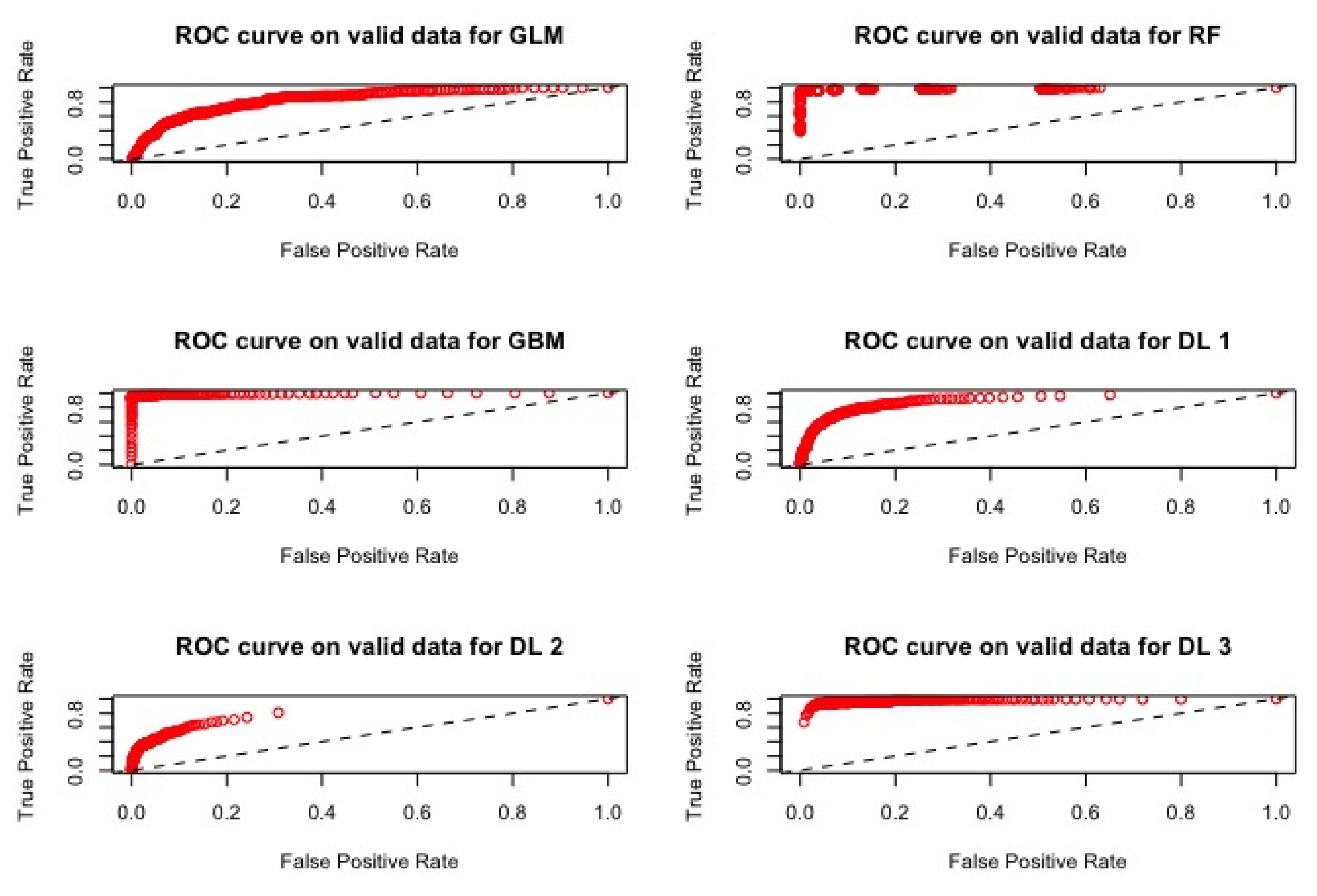
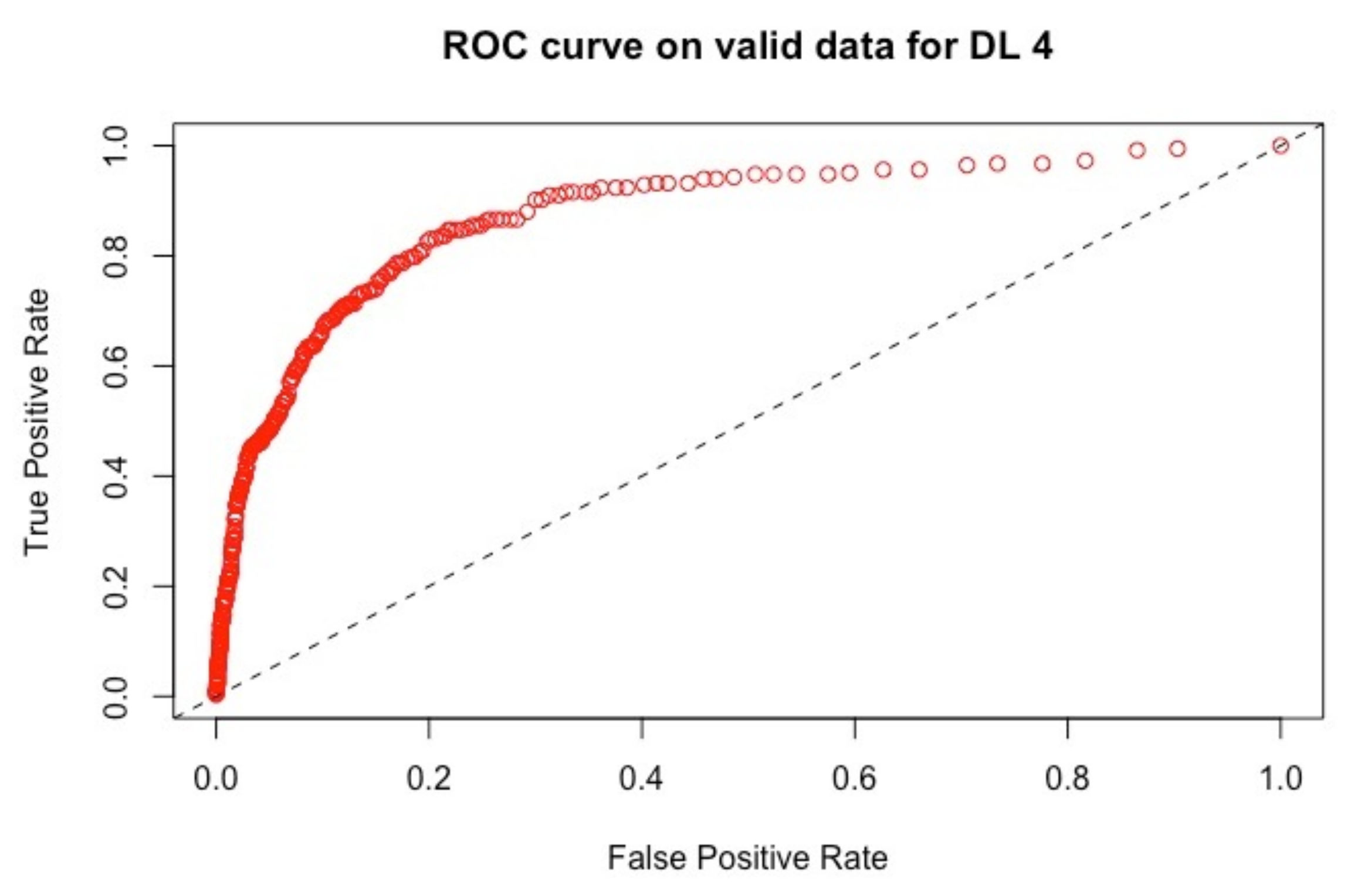
On the validation set, we observe that the AUC criteria have the highest value with model M3, then model M2, then model D3, and for the four last places, the model D1, then D4, M1 and D2. If we consider the RMSE criteria, the model M3 provides the smallest error, then the model M2, then D1 and D4 and, finally, D2, M1 and D3. Thus, the model D3 has the highest error. We observe that the ranking of the performance metric is not the same using the AUC and RMSE criteria.
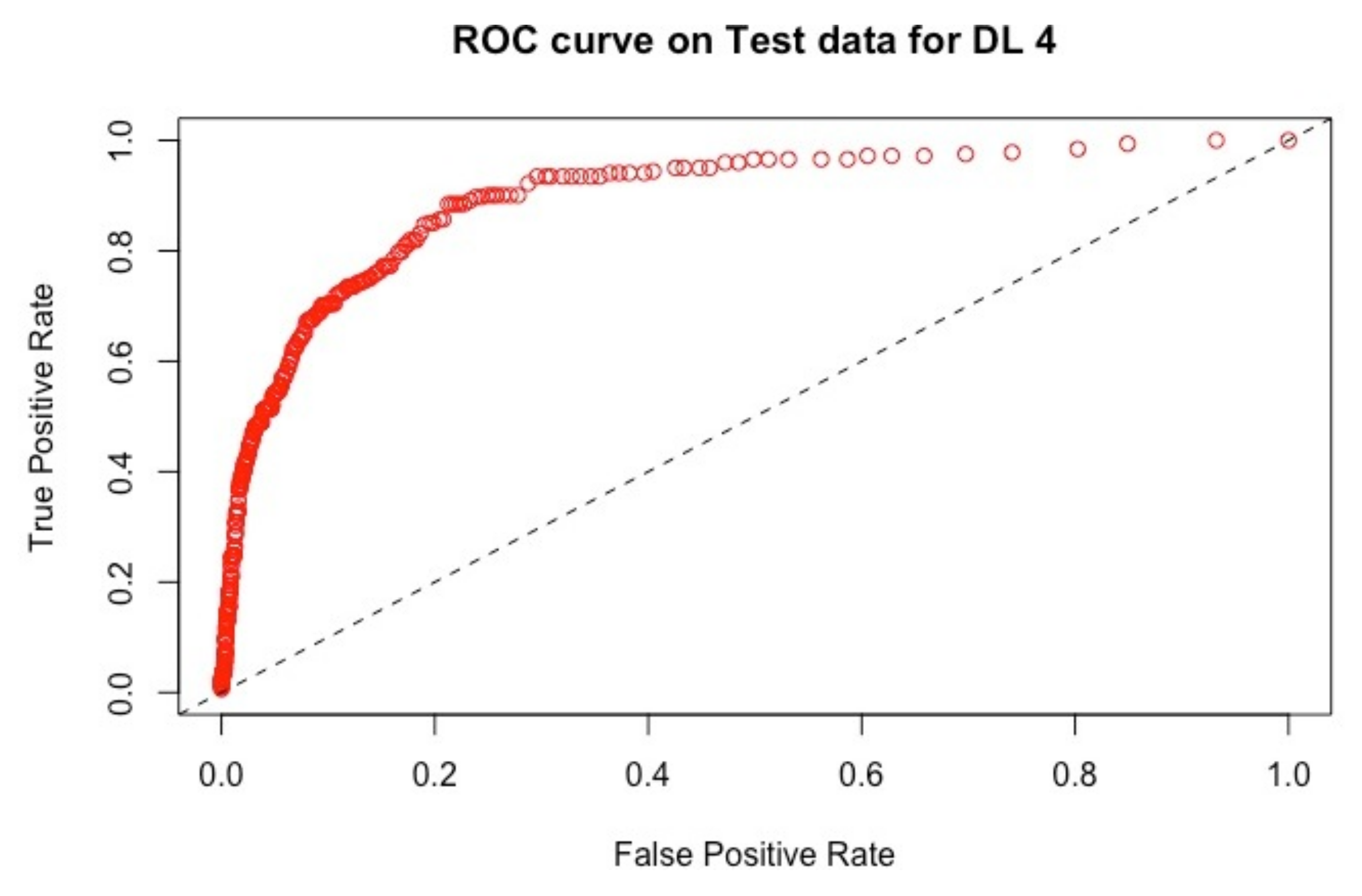
On the test set, we observe the same ranking for the AUC and for RMSE as with the training set, except for D1 and D4 that switch between the third and the fourth place. D3 provides the highest AUC among the deep learning models; however, it yields the highest error.
If the gradient boosting model remains the best fit (using the AUC) with the smallest error, we observe the stability of models on both the validation and test sets. In all scenarios, we observe that the deep learning models do not outperform the tree-based models (M2, M3). The comparison between the results obtained with the AUC criteria and the RMSE criteria indicate that a unique criterion is not sufficient.
The ROC curves corresponding to these results are provided in Figure 1, Figure 2, Figure 3 and Figure 4: they illustrate the speed at which the ROC curve attains the value of one on the y-axis with respect to the value of the specificity. The best curve can be observed on the second row and first column for the validation set in Figure 1 and for the test in Figure 3, which corresponds to the model M3.
Models M1–M3 and D1–D4 have all used the same 181 variables for fittings. In terms of variable importance, we do not obtain the same top 10 variables for all the models Gedeon (1997). The top 10 variables’ importance for the models are presented in Table 3 and correspond to 57 different variables. We refer to them as (they represent a subset of the original variables . Some variables are used by several algorithms, but in not more than three occurrences. Table 4 provides a brief description of some of the variables.
We now investigate the performance of these algorithms using only the 10 variables selected by each algorithm. We do then the same for the seven models. The results for the criteria AUC and RMSE are provided in Table 5, Table 6, Table 7, Table 8, Table 9, Table 10 and Table 11. Only the results obtained with the test set are provided.
All the tables showed similar results. The M2 and M3 models performed significantly bettercompared to the other five models in terms of the AUC. The deep learning models and the based logistic model poorly performed on these new datasets. Now, looking at the RMSE for the two best models, M3 is the best in all cases. The highest AUC and lowest RMSE among the seven models on these datasets is provided by the M3 model using the M3 top variables (Table 7).
Comparing the results provided by the best model using only the top 10 variables with the model fitted using the whole variable set (181 variables), we observe that the M3 model is the best in terms of highest AUC and smallest RMSE. The tree-based models provide stable results, whatever the number of variables used, which is not the case when we fit the deep learning models. Indeed, if we look at their performance when they use their top ten variables, this one is very poor: refer to Line 4 in Table 8, Line 5 in Table 9, Line 6 in Table 10 and Line 7 in Table 11.
In summary, the class of tree-based algorithms (M2 and M3) outperforms. In terms of the AUC and RMSE, the logistic regression model (M1) and the multilayer neural network models (deep learning D1–D4)) considered in this study in both the validation and test datasets using all 181 features, we observe that the gradient boosting model (M3) demonstrated high performance for the binary classification problem compared to the random forest model (M2), given the lower RMSE values.
Upon the selection of the top 10 variables from each model to be used for modeling, we obtain the same conclusion of higher performance with models M2 and M3, with M3 as the best classifier in terms of both the AUC and RMSE. The gradient boosting model (M3) recorded the highest performance on the test dataset in the top 10 variables selected out of the 181 variables by this model M3.
Now, we look at the profile of the top 10 variables selected by each model. We denote , the variables chosen by the models among the 181 original variables; we refer to Table 3 and Table 4. In this last table, we provide information on the variables that have been selected for this exercise. For instance, model M2 selects three variables already provided by model M1. Model M3 selects only one variable provided by model M1. The model D1 uses three variables of model M1. The model D2 selects one variable selected by model M2. Model D3 selects one variable used by model D1. The model D4 selects one variable selected by M1.
The classification of the variables used by each model is as follows: the variables of the model M1 correspond to flow data and aggregated balance sheets (assets and liabilities). As concerns financial statement data, the model M2 selects financial statement data and detailed financial statements (equities and debt). The model M3 selects detailed financial statements (equities and debt). The model D1 selects financial statement data and at the lowest level of granularity of financial statement data (long-term bank debt). The models D2 and D3 select an even lower level of granularity of financial statement data (short-term bank debt and leasing). The model D4 has selected the most granular data, for instance the ratio between elements as the financial statements.
Thus, we observe an important difference in the way the models select and work with the data they consider for scoring a company and as a result accepting to provide them with a loan. The model M1 selects more global and aggregated financial variables. The models M2 and M3 select detailed financial variables. The models relying on deep learning select more granular financial variables, which provide more detailed information on the customer. There is no appropriate discrimination among the deep learning models of selected variables and associated performance on the test set. It appears that the model M3 is capable of distinguishing the information provided by the data and only retains the information that improves the fit of the model. The tree-based models, M2 and M3, turn out to be the best and stable binary classifiers as they properly create split directions, thus keeping only the efficient information. From an economic stand point, the profile of the selected top 10 variables from the model M3 will be essential in deciding whether to provide a loan or not.
5. Conclusions
The rise of Big Data and data science approaches, such as machine learning and deep learning models, does have a significant role in credit risk modeling. In this exercise, we have showed that it is important to make checks on data quality (in the preparation and cleaning process to omit redundant variables), and it is important to deal with an imbalanced training dataset to avoid bias to a majority class.
We have also indicated that the choice of the features to respond to a business objective (In our case, should a loan be awarded to an enterprise? Can we use few variables to save time in this decision making?) and the choice of the algorithm used to make the decision (whether the enterprise makes defaults) are two important keys in the decision management processing when issuing a loan (here, the bank). These decisions can have an important impact on the real economy or the social world; thus, regular and frequent training of employees in this new field is crucial to be able to adapt to and properly use these new techniques. As such, it is important that regulators and policy-makers make quick decisions to regulate the use of data science techniques to boost performance, avoid discrimination in terms of wrong decisions proposed by algorithms and to understand the limits of some of these algorithms.
Additionally, we have shown that it is important to consider a pool of models that match the data and business problem. This is clearly deduced by looking at the difference in performance metrics. Note that we did not consider a combination of the different models. Data experts or data scientists need to be knowledgeable about the model structures (in terms of the choice of hyper-parameters, estimation, convergence criteria and performance metrics) in the modeling process. We recommend that performance metrics should not be only limited to one criterion like the AUC to enhance the transparency of the modeling process (see Kenett and Salini (2011)). It is important to note that standard criteria like the AIC, Bayesian information criterion (BIC) and R2 are not always suitable for the comparison of model performance, given the types of model classes (regression based, classification based, etc.). We also noticed that the use of more hyper-parameters, as in the grid deep learning model, does not outperform the tree-based models on the test dataset. Thus, practitioners need to be very skilled in modeling techniques and careful while using some black-box tools.
We have shown that the selection of the 10 top variables, based on the variable importance of models, does not necessarily yield stable results given the underlying model. Our strategy of re-checking model performance on these top variables can help data experts validate the choice of models and variables selected. In practice, requesting a few lists of variables from clients can help speed up the time to deliver a decision on a loan request.
We have seen that algorithms based on artificial neural networks do not necessarily provide the best performance and that regulators need also to ensure the transparency of decision algorithms to avoid discrimination in and a possible negative impact on the industry.
Acknowledgments
This work was achieved through the Laboratory of Excellence on Financial Regulation (LabEx ReFi) under the reference ANR-10-LABX-0095. It benefited from French government support managed by the National Research Agency (ANR) within the project Investissements d’Avenir Paris Nouveaux Mondes (Investments for the Future Paris-New Worlds) under the reference ANR-11-IDEX-0006-02. The authors would like to thank the anonymous reviewers for their valuable comments and suggestions to improve the quality of the paper. Peter Martey Addo, a former Lead Data Scientist and Expert Synapses at SNCF, would also like to thank his former colleagues of the Data Cluster for their valuable comments and suggestions.
Author Contributions
Peter Martey Addo, Dominique Guégan and Bertrand Hassani conceived of and designed the experiments. Peter Martey Addo performed the experiments by coding. All authors contributed to reagents/materials/analysis tools, as well as data and results analysis. Peter Martey Addo and Dominique Guégan ensured the methodological consistency. All authors wrote the paper.
Conflicts of Interest
The authors declare no conflicts of interest. The findings, interpretations, opinions and conclusions expressed herein are those of the authors and do not necessarily reflect the view of their respective institutional affiliations.
References
- Angelini, Eliana, Giacomo di Tollo, and Andrea Roli. 2008. A neural network approach for credit risk evaluation. The Quarterly Review of Economics and Finance 48: 733–55. [Google Scholar] [CrossRef]
- Anisha Arora, Arno Candel, Jessica Lanford, Erin LeDell, and Viraj Parmar. 2015. The Definitive Performance Tuning Guide for H2O Deep Learning. Leghorn St. Mountain View, CA, USA: H2O.ai, Inc. [Google Scholar]
- Bahrammirzaee, Arash. 2010. A comparative survey of artificial intelligence applications in finance: Artificial neural networks, expert system and hybrid intelligent systems. Neural Computing and Applications 19: 1165–95. [Google Scholar] [CrossRef]
- Balzer, Robert. 1985. A 15 year perspective on automatic programming. IEEE Transactions on Software Engineering 11: 1257–68. [Google Scholar] [CrossRef]
- Biau, Gérard. 2012. Analysis of a random forests model. Journal of Machine Learning Research 13: 1063–95. [Google Scholar]
- Breiman, Leo. 2000. Some Infinity Theory for Predictors Ensembles. Technical Report. Berkeley: UC Berkeley, vol. 577. [Google Scholar]
- Breiman, Leo. 2004. Consistency for a Sample Model of Random Forests. Technical Report 670. Berkeley: UC Berkeley, vol. 670. [Google Scholar]
- Butaru, Florentin, Qingqing Chen, Brian Clark, Sanmay Das, Andrew W. Lo, and Akhtar Siddique. 2016. Risk and risk management in the credit card industry. Journal of Banking and Finance 72: 218–39. [Google Scholar] [CrossRef]
- Ling, Charles X., and Chenghui Li. 1998. Data Mining for Direct Marketing Problems and Solutions. Paper presented at International Conference on Knowledge Discovery from Data (KDD 98). New York City, August 27–31; pp. 73–79. [Google Scholar]
- Chawla, Nitesh V., Kevin W. Bowyer, Lawrence O. Hall, and W. Philip Kegelmeyer. 2002. Smote: Synthetic minority over-sampling technique. Journal of Artificial Intelligence Research 16: 321–57. [Google Scholar]
- CNIL. 2017. La loi pour une république numérique: Concertation citoyenne sur les enjeux éthiques lies à la place des algorithmes dans notre vie quotidienne. In Commission nationale de l’informatique et des libertés. Montpellier: CNIL. [Google Scholar]
- Deville, Yves, and Kung-Kiu Lau. 1994. Logic program synthesis. Journal of Logic Programming 19: 321–50. [Google Scholar] [CrossRef]
- Pierre Geurts, Damien Ernst, and Louis Wehenkel. 2006. Extremely randomized trees. Machine Learning 63: 3–42. [Google Scholar] [CrossRef]
- Fan, Jianqing, and Runze Li. 2001. Variable selection via nonconcave penalized likelihood and its oracle properties. Journal of the American Statistical Society 96: 1348–60. [Google Scholar] [CrossRef]
- Friedman, Jerome, Trevor Hastie, and Rob Tibshirani. 2001. The elements of statistical learning. Springer Series in Statistics 1: 337–87. [Google Scholar]
- Friedman, Jerome, Trevor Hastie, and Rob Tibshirani. 2010. Regularization paths for generalized linear models via coordinate descent. Journal of Statistical Software 33: 1. [Google Scholar] [CrossRef] [PubMed]
- Friedman, Jerome H. 2001. Greedy function approximation: A gradient boosting machine. The Annals of Statistics 29: 1189–232. [Google Scholar] [CrossRef]
- Galindo, Jorge, and Pablo Tamayo. 2000. Credit risk assessment using statistical and machine learning: Basic methodology and risk modeling applications. Computational Economics 15: 107–43. [Google Scholar] [CrossRef]
- Gastwirth, Joseph L. 1972. The estimation of the lorenz curve and the gini index. The Review of Economics and Statistics 54: 306–16. [Google Scholar] [CrossRef]
- GDPR. 2016. Regulation on the Protection of Natural Persons with Regard to the Processing of Personal Data and on the Free Movement of Such Data, and Repealing Directive 95/46/EC (General Data Protection Regulation). EUR Lex L119. Brussels: European Parliament, pp. 1–88. [Google Scholar]
- Gedeon, Tamás D. 1997. Data mining of inputs: Analyzing magnitude and functional measures. International Journal of Neural Systems 8: 209–17. [Google Scholar] [CrossRef] [PubMed]
- Genuer, Robin, Jean-Michel Poggi, and Christine Tuleau. 2008. Random Forests: Some Methodological Insights. Research Report RR-6729. Paris: INRIA. [Google Scholar]
- Hinton, Geoffrey E., and Ruslan R. Salakhutdinov. 2006. Reducing the dimensionality of data with neural networks. Science 313: 504–7. [Google Scholar] [CrossRef] [PubMed]
- Siegelmann, Hava T., and Eduardo D. Sontag. 1991. Turing computability with neural nets. Applied Mathematics Letters 4: 77–80. [Google Scholar] [CrossRef]
- Huang, Zan, Hsinchun Chen, Chia-Jung Hsu, Wun-Hwa Chen, and Soushan Wu. 2004. Credit rating analysis with support vector machines and neural networks: A market comparative study. Decision Support Systems 37: 543–58. [Google Scholar] [CrossRef]
- Kenett, Ron S., and Silvia Salini. 2011. Modern analysis of customer surveys: Comparison of models and integrated analysis. Applied Stochastic Models in Business and Industry 27: 465–75. [Google Scholar] [CrossRef]
- Khandani, Amir E., Adlar J. Kim, and Andrew W. Lo. 2010. Consumer credit-risk models via machine-learning algorithms. Journal of Banking and Finance 34: 2767–87. [Google Scholar] [CrossRef] [Green Version]
- Kubat, Miroslav, Robert C. Holte, and Stan Matwin. 1999. Machine learning in the detection of oil spills in satellite radar images. Machine Learning 30: 195–215. [Google Scholar] [CrossRef]
- Kubat, Miroslav, and Stan Matwin. 1997. Addressing the curse of imbalanced training sets: One sided selection. Paper presented at Fourteenth International Conference on Machine Learning. San Francisco, CA, USA, July 8–12; pp. 179–186. [Google Scholar]
- Lerman, Robert I., and Shlomo Yitzhaki. 1984. A note on the calculation and interpretation of the gini index. Economic Letters 15: 363–68. [Google Scholar] [CrossRef]
- Menardi, Giovanna, and Nicola Torelli. 2011. Training and assessing classification rules with imbalanced data. Data Mining and Knowledge Discovery 28: 92–122. [Google Scholar] [CrossRef]
- Mladenic, Dunja, and Marko Grobelnik. 1999. Feature selection for unbalanced class distribution and naives bayes. Paper presented at 16th International Conference on Machine Learning. San Francisco, CA, USA, June 27–30; pp. 258–267. [Google Scholar]
- Raileanu, Laura Elena, and Kilian Stoffel. 2004. Theoretical comparison between the gini index and information gain criteria. Annals of Mathematics and Artificial Intelligence 41: 77–93. [Google Scholar] [CrossRef]
- Schmidhuber, Jurgen. 2014. Deep Learning in Neural Networks: An Overview. Technical Report IDSIA-03-14. Lugano: University of Lugano & SUPSI. [Google Scholar]
- Schölkopf, Bernhard, Christopher J. C. Burges, and Alexander J. 1998. Advances in Kernel Methods—Support Vector Learning. Cambridge: MIT Press, vol. 77. [Google Scholar]
- Seetharaman, A, Vikas Kumar Sahu, A. S. Saravanan, John Rudolph Raj, and Indu Niranjan. 2017. The impact of risk management in credit rating agencies. Risks 5: 52. [Google Scholar] [CrossRef]
- Sirignano, Justin, Apaar Sadhwani, and Kay Giesecke. 2018. Deep Learning for Mortgage Risk. Available online: https://ssrn.com/abstract=2799443 (accessed on 9 February 2018).
- Tibshirani, Robert. 1996. Regression shrinkage and selection via the lasso. Journal of the Royal Statistical Society, Series B 58: 267–88. [Google Scholar]
- Tibshirani, Robert. 2011. Regression shrinkage and selection via the lasso:a retrospective. Journal of the Royal Statistical Society, Series B 58: 267–88. [Google Scholar]
- Vapnik, Vladimir. 1995. The Nature of Statistical Learning Theory. Berlin: Springer. [Google Scholar]
- Yitzhaki, Shlomo. 1983. On an extension of the gini inequality index. International Economic Review 24: 617–28. [Google Scholar] [CrossRef]
- Zou, Hui. 2006. The adaptive lasso and its oracle properties. Journal of the American Statistical Society 101: 1418–29. [Google Scholar] [CrossRef]
- Zou, Hui, and Trevor Hastie. 2005. Regulation and variable selection via the elastic net. Journal of the Royal Statistical Society 67: 301–20. [Google Scholar] [CrossRef]
| 1. | There exist a lot of other references concerning Lasso models; thus, this introduction does not consider all the problems that have been investigated concerning this model. We provide some more references noting that most of them do not have the same objectives as ours. The reader can read with interest Fan and Li (2001), Zhou (2006) and Tibschirani (2011). |
| 2. | Here, T stands for transpose |
| 3. | As soon as the AUC is known, the Gini index can be obtained under specific assumptions |
| 4. | In medicine, it corresponds to the probability of the true negative |
| 5. | In medicine, corresponding to the probability of the true positive |
| 6. | The code implementation in this section was done in ‘R’. The principal package used is H2o.ai Arno et al. (2015). The codes for replication and implementation are available at https://github.com/brainy749/CreditRiskPaper. |
Figure 1.
ROC curves for the models M1, M2, M3, D1, D2 and D3 using 181 variables using the validation set.
Figure 1.
ROC curves for the models M1, M2, M3, D1, D2 and D3 using 181 variables using the validation set.

Figure 2.
ROC curve for the model D4 using 181 variables using the validation set.

Figure 3.
ROC curves for the models M1, M2, M3, D1, D2 and D3 using 181 variables with the test set.
Figure 3.
ROC curves for the models M1, M2, M3, D1, D2 and D3 using 181 variables with the test set.
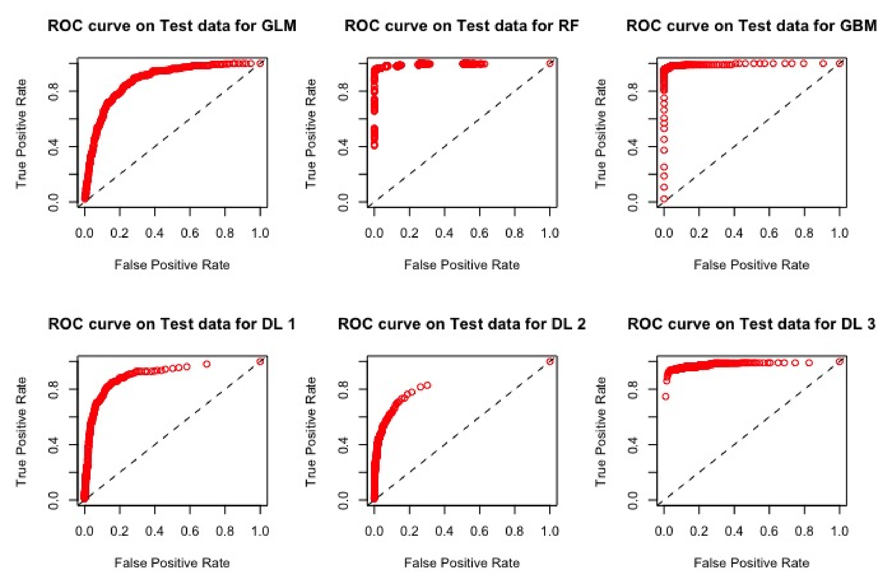
Figure 4.
ROC curve for the model D4 using 181 variables with the test set.


Table 1.
Models’ performances on the validation dataset with 181 variables using AUC and RMSE values for the seven models.
Table 1.
Models’ performances on the validation dataset with 181 variables using AUC and RMSE values for the seven models.
| Models | AUC | RMSE |
|---|---|---|
| M1 | 0.842937 | 0.247955 |
| M2 | 0.993271 | 0.097403 |
| M3 | 0.994206 | 0.041999 |
| D1 | 0.902242 | 0.120964 |
| D2 | 0.812946 | 0.124695 |
| D3 | 0.979357 | 0.320543 |
| D4 | 0.877501 | 0.121133 |
Table 2.
Models’ performances on the test dataset with 181 variables using AUC and RMSE values for the seven models.
Table 2.
Models’ performances on the test dataset with 181 variables using AUC and RMSE values for the seven models.
| Models | AUC | RMSE |
|---|---|---|
| M1 | 0.876280 | 0.245231 |
| M2 | 0.993066 | 0.096683 |
| M3 | 0.994803 | 0.044277 |
| D1 | 0.904914 | 0.114487 |
| D2 | 0.841172 | 0.116625 |
| D3 | 0.975266 | 0.323504 |
| D4 | 0.897737 | 0.113269 |
Table 3.
Top 10 variables selected by the seven models.
| M1 | M2 | M3 | D1 | D2 | D3 | D4 | |
|---|---|---|---|---|---|---|---|
| X1 | A1 | A11 | A11 | A25 | A11 | A41 | A50 |
| X2 | A2 | A5 | A6 | A6 | A32 | A42 | A7 |
| X3 | A3 | A2 | A17 | A26 | A33 | A43 | A51 |
| X4 | A4 | A1 | A18 | A27 | A34 | A25 | A52 |
| X5 | A5 | A9 | A19 | A7 | A35 | A44 | A53 |
| X6 | A6 | A12 | A20 | A28 | A36 | A45 | A54 |
| X7 | A7 | A13 | A21 | A29 | A37 | A46 | A55 |
| X8 | A8 | A14 | A22 | A1 | A38 | A47 | A56 |
| X9 | A9 | A15 | A23 | A30 | A39 | A48 | A57 |
| X10 | A10 | A16 | A24 | A31 | A40 | A49 | A44 |
Table 4.
Example of variables used in the models, where ’EBITDA’ denotes Earnings Before Interest, Taxes, Depreciation and Amortization; ’ABS’ denotes Absolute Value function; ’LN’ denotes Natural logarithm.
Table 4.
Example of variables used in the models, where ’EBITDA’ denotes Earnings Before Interest, Taxes, Depreciation and Amortization; ’ABS’ denotes Absolute Value function; ’LN’ denotes Natural logarithm.
| TYPE | METRIC |
|---|---|
| EBITDA | EBITDA/FINACIAL EXPENSES |
| EBITDA/Total ASSETS | |
| EBITDA/EQUITY | |
| EBITDA/SALES | |
| EQUITY | EQUITY/TOTAL ASSETS |
| EQUITY/FIXED ASSETS | |
| EQUITY/LIABILITIES | |
| LIABILITIES | LONG-TERM LIABILITIES/TOTAL ASSETS |
| LIABILITIES/TOTAL ASSETS | |
| LONG TERM FUNDS/FIXED ASSETS | |
| RAW FINANCIALS | LN (NET INCOME) |
| LN(TOTAL ASSETS) | |
| LN (SALES) | |
| CASH-FLOWS | CASH-FLOW/EQUITY |
| CASH-FLOW/TOTAL ASSETS | |
| CASH-FLOW/SALES | |
| PROFIT | GROSS PROFIT/SALES |
| NET PROFIT/SALES | |
| NET PROFIT/TOTAL ASSETS | |
| NET PROFIT/EQUITY | |
| NET PROFIT/EMPLOYEES | |
| FLOWS | (SALES (t) −SALES (t−1))/ABS(SALES (t−1)) |
| (EBITDA (t) −EBITDA (t−1))/ABS(EBITDA (t−1)) | |
| (CASH-FLOW (t) −CASH-FLOW (t−1))/ABS(CASH-FLOW (t−1)) | |
| (EQUITY (t) − EQUITY (t−1))/ABS(EQUITY (t−1)) |
Table 5.
Performance for the seven models using the top 10 features from model M1 on the test dataset.
Table 5.
Performance for the seven models using the top 10 features from model M1 on the test dataset.
| Models | AUC | RMSE |
|---|---|---|
| M1 | 0.638738 | 0.296555 |
| M2 | 0.98458 | 0.152238 |
| M3 | 0.975619 | 0.132364 |
| D1 | 0.660371 | 0.117126 |
| D2 | 0.707802 | 0.119424 |
| D3 | 0.640448 | 0.117151 |
| D4 | 0.661925 | 0.117167 |
Table 6.
Performance for the seven models using the top 10 features from model M2 on the test dataset.
Table 6.
Performance for the seven models using the top 10 features from model M2 on the test dataset.
| Models | AUC | RMSE |
|---|---|---|
| M1 | 0.595919 | 0.296551 |
| M2 | 0.983867 | 0.123936 |
| M3 | 0.983377 | 0.089072 |
| D1 | 0.596515 | 0.116444 |
| D2 | 0.553320 | 0.117119 |
| D3 | 0.585993 | 0.116545 |
| D4 | 0.622177 | 0.878704 |
Table 7.
Performance for the seven models using the top 10 features from model M3 on the test dataset.
Table 7.
Performance for the seven models using the top 10 features from model M3 on the test dataset.
| Models | AUC | RMSE |
|---|---|---|
| M1 | 0.667479 | 0.311934 |
| M2 | 0.988521 | 0.101909 |
| M3 | 0.992349 | 0.077407 |
| D1 | 0.732356 | 0.137137 |
| D2 | 0.701672 | 0.116130 |
| D3 | 0.621228 | 0.122152 |
| D4 | 0.726558 | 0.120833 |
Table 8.
Performance for the seven models using the top 10 features from model D1 on the test dataset.
Table 8.
Performance for the seven models using the top 10 features from model D1 on the test dataset.
| Models | AUC | RMSE |
|---|---|---|
| M1 | 0.669498 | 0.308062 |
| M2 | 0.981920 | 0.131938 |
| M3 | 0.981107 | 0.083457 |
| D1 | 0.647392 | 0.119056 |
| D2 | 0.667277 | 0.116790 |
| D3 | 0.6074986 | 0.116886 |
| D4 | 0.661554 | 0.116312 |
Table 9.
Performance for the seven models using the top 10 features from model D2 on the test dataset.
Table 9.
Performance for the seven models using the top 10 features from model D2 on the test dataset.
| Models | AUC | RMSE |
|---|---|---|
| M1 | 0.669964 | 0.328974 |
| M2 | 0.989488 | 0.120352 |
| M3 | 0.983411 | 0.088718 |
| D1 | 0.672673 | 0.121265 |
| D2 | 0.706265 | 0.118287 |
| D3 | 0.611325 | 0.117237 |
| D4 | 0.573700 | 0.116588 |
Table 10.
Performance for the seven models using the top 10 features from model D3 on the test dataset.
Table 10.
Performance for the seven models using the top 10 features from model D3 on the test dataset.
| Models | AUC | RMSE |
|---|---|---|
| M1 | 0.640431 | 0.459820 |
| M2 | 0.980599 | 0.179471 |
| M3 | 0.985183 | 0.112334 |
| D1 | 0.712025 | 0.158077 |
| D2 | 0.838344 | 0.120950 |
| D3 | 0.753037 | 0.117660 |
| D4 | 0.711824 | 0.814445 |
Table 11.
Performance for the seven models using the top 10 features from model D4 on the test dataset.
Table 11.
Performance for the seven models using the top 10 features from model D4 on the test dataset.
| Models | AUC | RMSE |
|---|---|---|
| M1 | 0.650105 | 0.396886 |
| M2 | 0.985096 | 0.128967 |
| M3 | 0.984594 | 0.089097 |
| D1 | 0.668186 | 0.116838 |
| D2 | 0.827911 | 0.401133 |
| D3 | 0.763055 | 0.205981 |
| D4 | 0.698505 | 0.118343 |
© 2018 by the authors. Licensee MDPI, Basel, Switzerland. This article is an open access article distributed under the terms and conditions of the Creative Commons Attribution (CC BY) license (http://creativecommons.org/licenses/by/4.0/).
Share and Cite
MDPI and ACS Style
Addo, P.M.; Guegan, D.; Hassani, B. Credit Risk Analysis Using Machine and Deep Learning Models. Risks 2018, 6, 38. https://doi.org/10.3390/risks6020038
AMA Style
Addo PM, Guegan D, Hassani B. Credit Risk Analysis Using Machine and Deep Learning Models. Risks. 2018; 6(2):38. https://doi.org/10.3390/risks6020038
Chicago/Turabian StyleAddo, Peter Martey, Dominique Guegan, and Bertrand Hassani. 2018. "Credit Risk Analysis Using Machine and Deep Learning Models" Risks 6, no. 2: 38. https://doi.org/10.3390/risks6020038
Note that from the first issue of 2016, this journal uses article numbers instead of page numbers. See further details here.