Life Insurance and Annuity Demand under Hyperbolic Discounting


1
The QSuper Group, 70 Eagle Street, Brisbane, QLD 4000, Australia
2
Department of Actuarial Studies and Business Analytics, Faculty of Business and Economics, Macquarie University, Sydney, NSW 2109, Australia
*
Author to whom correspondence should be addressed.
†
These authors contributed equally to this work.
Risks 2018, 6(2), 43; https://doi.org/10.3390/risks6020043
Submission received: 29 March 2018
/
Revised: 12 April 2018
/
Accepted: 17 April 2018
/
Published: 23 April 2018
(This article belongs to the Special Issue Optimal Demands for Life Insurance and Annuities)
Abstract
:In this paper, we analyse and construct a lifetime utility maximisation model with hyperbolic discounting. Within the model, a number of assumptions are made: complete markets, actuarially fair life insurance/annuity is available, and investors have time-dependent preferences. Time dependent preferences are in contrast to the usual case of constant preferences (exponential discounting). We find: (1) investors (realistically) demand more life insurance after retirement (in contrast to the standard model, which showed strong demand for life annuities), and annuities are rarely purchased; (2) optimal consumption paths exhibit a humped shape (which is usually only found in incomplete markets under the assumptions of the standard model).
1. Introduction
With the declining mortality rates, life expectancy has been improved over the last few decades and is one key driver of the ageing population all over the world (World Health Organization 2015). Retirees with longer life expectancy are increasingly exposed to longevity risk.
Improved life expectancy can generate more financial burden for governments that provide social security. Retirees who pursue financial sustainability of their retirement benefits can share this burden by purchasing an annuity to self-insure (Oppers et al. 2012). The works of Yaari (1965) and Merton (1969) suggest that investors can hedge longevity risk and further financially benefit themselves by purchasing annuities.
However, low demand for voluntary annuitisation is observed among people, and is known as the annuity puzzle. Numerous explanations for this annuity puzzle have been provided in the literature. The bequest motive was offered as one explanation for the annuity puzzle in Friedman and Warshawsky (1990) and Bernheim (1991). Lockwood (2012), examining empirical data, further found that bequest motives have characteristics akin to luxury goods. Finkelstein and Poterba (2004) suggested that adverse selection1 could reduce demand in the voluntary annuity market. Bütler et al. (2017) found that the means test in a social security system can impact annuitisation levels, also shedding light on the annuity puzzle.
The contribution of this paper is that the time-inconsistent behaviour of investors can also be seen as contributing to low voluntary annuity demand. Strotz (1955) points out that the preferences of an individual are time-inconsistent due to their dynamic nature. Hence, investors might not be interested in investing in a long-term financial contract, like an annuity. In economic terms, hyperbolic discounting implies that the rate of time preference is no longer constant, but is a function of time. The traditional exponential discounting approach is then a special case of this, where the rate of time preference is held constant.
Most of the benchmark intertemporal decision-making models use constant exponential discounting, consumption and investment literature. The classical problem of this type is Merton’s model (Merton 1969), where explicit optimal formulae for consumption and portfolio rules under constant relative risk averse (CRRA) utility are obtained. Richard (1975) further generalized Merton’s model by adding a bequest utility function. The bequest utility function has an important implication: generating demand for insurance and annuities. Pliska and Ye (2007) extended Richard’s model by allowing an unbounded lifetime. Zhang et al. (2017) applied Richard’s model to an optimal stopping problem concerning entry into a retirement village. This work of Merton and Richard has answered the question of optimal demand for life insurance and annuities under the assumption of complete markets, rational consumers and exponential discounting.
The hyperbolic discount rate predicates time-inconsistent preferences, which are well documented in the literature. Time-inconsistent preferences of an investor were treated in Strotz (1955) as the consequence of dynamic behaviour. In further studying those dynamic behaviors, Pollak (1968) separated the dynamic behaviours into two groups: naïve and sophisticated. In Pollak (1968), naïve investors were defined as the people who never realise the nature of their dynamic behavior; sophisticated investors were defined as the people who do realise the nature of their dynamic behaviour.
Naïve agents have no commitment technology or commitment mechanism. With a non-constant rate of time preference a problem arises because the relative valuation of utility flows at different dates changes as the planning date evolves. Without a commitment technology/mechanism, there is no way that agents can follow an initially chosen consumption path, as it differs from that which would be chosen sequentially. Naïve agents are unable to follow such initially chosen paths, and their consumption evolves purely sequentially. Compared to naïve agents, sophisticated agents recognise their time inconsistent preferences and adopt a consistent plan—that is, they have a commitment technology/mechanism that enables them to follow a committed chosen consumption path, in spite of the fact that it differs from that which would be chosen sequentially.
Exploring a more general optimal consumption and investment model, Marín-Solano and Navas (2010) utilised hyperbolic discounting for both naïve and sophisticated investors within the framework of Merton’s model. Analytical results were then obtained for both cases, but in a framework absent of life insurance and life annuities. Drawing on Marín-Solano and Navas (2010), we complete the modelling of life insurance and annuities. We further study the naïve case with bequest motives under Richard’s framework and find the behavior of naïve agents and real world insurance and annuity consumers are very much alike. While we also treat the sophisticated case, generating results for such agents is more complicated as no closed form solution is possible. We leave its results to future research, and note, by its absence, that we are not considering the extremely strong-willed and well-informed members of the insurance and annuity buying public. This paper is structured as follows: Section 2 develops the the modelling, Section 3 presents the results, and Section 4 provides the conclusions.
2. Model
In Richard’s framework (Richard 1975), an agent at time t is assumed to maximise lifetime utility via appropriate choices of consumption, , proportion invested in risky asset, , and legacy level, . Here, we assume that the dynamics of the risky asset price available in the market, , is
where and are the return rate and volatility of , and is standard Brownian motion.
The agent’s death time is modelled by the force of mortality, , and survival rate, , with the density function of mortality, , defined as
Then, the insurance premium is . Positive insurance premiums imply that agents’ bequest motives exceed their wealth level. Hence, they purchase life insurance from an insurer to cover the gap between and . Negative insurance premiums imply agents’ wealth levels exceed their bequest motives. Hence, they purchase an annuity from an insurer to annuitise the gap between and .
Drawing on Purcal and Piggott (2008) and Marín-Solano and Navas (2010), with the hyperbolic preferences, the objective of an utility maximising agent with the mortality density function (1) is
subject to the dynamics of financial wealth W,
where U and Z are the utility functions for consumption and bequest, T is the uncertain time of death, W is the wealth level, is the discounting factor, is the limiting age, r is the risk free rate available in the market and Y is (deterministic) income. The hyperbolic discount rate, , and the discounting factor we use is adopted from Barro (1999),
where is the agent’s (constant) long run rate of time preference, is the degree of impatience and is the constant rate of decline in impatience. Note that becomes a constant exponential discounting factor when .
In this paper, utility functions are assumed to be CRRA with
where is the risk aversion parameter and is the “discount” function for bequest2. From Purcal and Piggott (2008), this “discount” function generates a bequest that provides a continuous annuity certain that commences at the time of the decease of the investor and ends at the limiting age, , of the life table, having assumed that the investor and spouse are the same age. Specifically, this continuous annuity is assumed to pay of the consumption level at the time when the investor dies,
2.1. Naïve Case
Let be the value function. Based on Marín-Solano and Navas (2010), the dynamic programming equation for the naïve agent with hyperbolic discounting is derived3 as follows:
With first-order conditions, we obtain the optimal consumption, portfolio rules, and legacy from (6), respectively
and
Interestingly, by comparing Equations (7) with (9), we see that the optimal legacy is actually the product of optimal consumption and the continuous annuity, , which fulfill our assumption above.
For a deterministic income stream Y, Richard (Richard 1975) demonstrates that the capitalisation of the income stream, , is and the total wealth, , is .
The problem faced by the investor ultimately becomes one of solving the partial differential equation for . Based on Richard (1975) and Purcal and Piggott (2008), the form of the solution is
As we expect, these results turn out to be very similar to the ones from Richard (1975) and Purcal and Piggott (2008). What we are most interested in is the realization of the path of these optimal controls throughout agent’s lifetime, which will be shown graphically in the next section.
2.2. Sophisticated Case
The sophisticated agents solve this optimal control problem via a backwards recursive induction approach. This approach solves the problem retrospectively to obtain the optimal control variables from terminal time backwards, which is also in line with the dynamic programming approach. The objective of the utility maximising sophisticated individual would be the same.
Even though the objective of the individual is the same for both naïve and sophisticated cases, the way to solve each problem differs. As noted above, naïve agents do not have any awareness of their time-inconsistent preferences that are changing from time to time. Sophisticated agents realise that their behaviour is time-inconsistent. Hence, they make decisions based on the equilibrium of a series of future behaviours (Marín-Solano and Navas 2010). This approach implicitly fulfills the (backwards) recursive induction approach, where equilibrium is found for the states conditioned on the behaviour of two successive players, denoted here as self 1 and self 2 (that is, the player, at two successive time points), or self 2 and self 3, or, etc.—hence generating a recursive relation between successive players. Say, for example, self 1 makes a decision based on the equilibrium of states conditioned on self 1 and self 2; self 2 would make a decision based on the equilibrium of states conditioned on self 2 and self 3—and continue in this fashion until terminal time. Hence, self 1 makes a decision based on all future equilibria indirectly through such recursive relations.
Let be the value function again. We follow Marín-Solano and Navas (2010) and their derivation of the modified dynamic programming equation, which found equilibrium in discrete time fashion, and then passed to the limit for the continuous time case. The modified dynamic programming equation for our extended model is derived5 and shown below:
where
We solve for the functional form of control and state variables by following exactly the same procedure as in Section 2.1 and obtain the optimal controls, which are also given by Equations (11)–(13). In contrast, now becomes the solution to the integro-differential equation
The above integro-differential equation needs to be solved numerically6.
3. Results
3.1. Parameter Values
The results we present are based on agents whose lifetimes are counted from age to a maximum age with assumed survival rates and force of mortality from Ministry of Health, Labour and Welfare (2010). Parameter values are summarised in Table 1.
Following Purcal and Piggott (2008), we used the Nikkei 225 return rates from 2005 to 20147 to calculate the risky asset return rate, , and volatility, . Based on the average yield rate of 10-year treasury bonds in 2015 from the Ministry of Finance, Japan, we set the risk-free rate to per annum. In addition, recent Japanese average monthly wage data from Ministry of Health, Labour and Welfare (2015) was used to calculate the annual income, Y = 5,102,412 yen, which is also assumed to be the agent’s initial wealth amount. In our model, an agent is assumed to receive a constant income stream of Y = 5,102,412 yen before retirement age (65), and have no income, , after retirement.
A traditional exponential discounting model would use a constant rate of time preference; its level could reasonably be set to that of the risk-free rate Purcal and Piggott (2008). Determining the hyperbolic discount factors is more involved. Laibson (1997) argues, to obtain empirically observed discount preferences, the parameter should be around 0.5 per annum while should be at least 0.5 per annum. Barro (1999) points out the value of a perpetuity to a hyperbolic discounter is
Now, the value to an exponential discounter with a rate of time preference of r of this same perpetuity is
and this suggests a calibration method for the hyperbolic discounting factors. Tang (2009) suggests it is not unreasonable to assume the exponential and hyperbolic discounters agree on the price of a perpetuity, and so . Taken together with the Laibson (1997) constraints, we can then solve for , and numerically—here we find , and .
3.2. Hyperbolic Discounting Results
Recall that within the discounting factor, , and determine the degree of impatience and the decline of the impatience effect, respectively. In addition to our calibrated values, we also present results for various values for these parameters.
To measure the impacts of the impatience degree on agent behaviour, we present a number of graphical illustrations of the expected consumption path and the expected insurance premium trajectories for different values in Figure 1 and Figure 2 and compare them to the behaviour of agents with exponential preferences (note that agents have exponential preferences and time-consistent behaviour when ).
From Figure 1, we can see that naïve agents who have higher values (the degree of impatience) consume more in the earlier stage of their life, then reduce their consumption substantially and end up with a relatively low level of consumption. In Figure 1, the consumption paths of naïve agents with hyperbolic discounting factor exhibit a humped shape for some values, even though the market is assumed to be complete and fair life insurance/annuities are available. Such humped shape consumption paths are usually observed in empirical data, as reported in Carroll (1997)8 and Gourinchas and Parker (2002)9. On the other hand, for agents with exponential preferences (i.e., ), the consumption paths exhibit a straight line manner for most of the life span of the investor—due to the existence of fair insurance/annuities and market completeness.
In our model, positive insurance premium indicates demand for life insurance and negative premium shows the demand for annuities. In Figure 2, agents with positive impatience degrees exhibit quite strong demand for life insurance as all premium trajectories are positive for the most of life. Before retirement (age 65), naïve agents with hyperbolic preferences would take life insurance contracts at an early age because they have insufficient financial wealth to service their desired bequest motive, while agents with exponential preferences have relatively lower demand for insurance and start to purchase annuities in their early 60s. At retirement (age 65), human capital has been fully transformed into financial wealth and transition from working to retirement occurs. Hence, kinks emerge for the premium paths. After retirement (age 65), agents’ financial wealth no longer accumulates from human capital. The expected insurance premium paths rise further for agents with a high impatience level. Meanwhile, the expected insurance premium paths start to decline for the agents with low impatience levels (including exponential preference agents), since they had lower consumption levels in the earlier stages of life, which later generated sufficient wealth. All agents reduce their demand for life insurance in the very late life stage, as they have adequate wealth to support their consumption at that time.
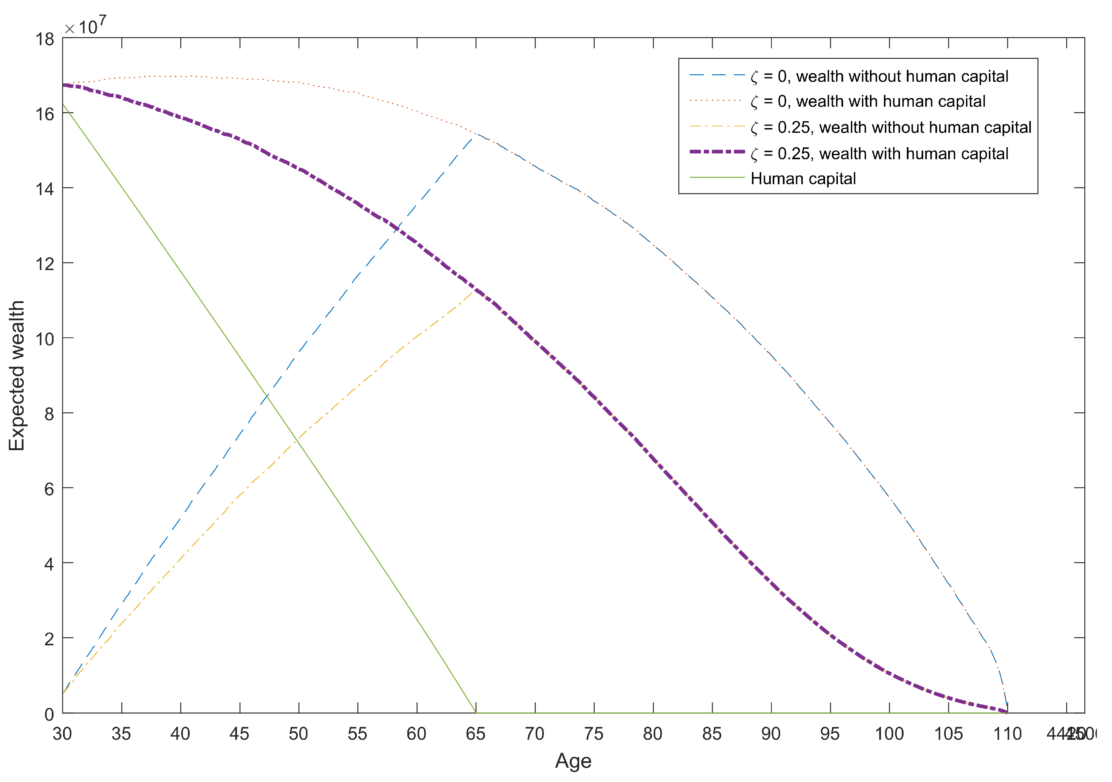
To further explore this difference in behaviours between naïve agents with hyperbolic preference and agents with exponential preferences, we plot the expected wealth paths for the exponential case and naïve case with in Figure 3. As discussed in the previous section, agents’ total wealth includes financial wealth and their capitalised future income stream (known as human capital). Human capital decreases with ageing and becomes zero when agents reach their retirement age. Agents with exponential preference possess higher expected trajectories in both total wealth and financial wealth, as naïve agents with hyperbolic preferences accumulate less wealth due to high consumption in the early life stage.
4. Conclusions
The hyperbolic discounting effect causes naïve agents to prefer immediate consumption, which hinders wealth accumulation at the early stage of life. Low levels of financial wealth constrain agents’ ability to fulfill their desired bequest motive; therefore, agents demand more life insurance, rather than an annuity, to fill this deficit.
We also found that humped shape consumption paths can be obtained in the hyperbolic discounting model under complete market assumptions. This result is in line with empirical observations.
These two results also serve to shed light on the annuity puzzle, as we see naïve agents will have low demand for voluntary annuities.
Numerical results on the annuity demand of sophisticated agents will be pursued in future research. Also of interest would be to treat agents with stochastic labour income as well as optimal financial decision-making for those with a mixture of exponential discounting and hyperbolic discounting structures.
Acknowledgments
The authors thank the reviewers for their valuable suggestions.
Author Contributions
Siqi Tang and Sachi Purcal conceived and designed the experiments. Siqi Tang and Jinhui Zhang performed the experiments. Siqi Tang, Sachi Purcal and Jinhui Zhang analysed the data. Siqi Tang and Jinhui Zhang wrote the paper.
Conflicts of Interest
The authors declare no conflict of interest.
References
- Barro, Robert J. 1999. Ramsey meets Laibson in the neoclassical growth model. The Quarterly Journal of Economics 114: 1125–52. [Google Scholar] [CrossRef]
- Bernheim, B. Douglas. 1991. How strong are bequest motives? Evidence based on estimates of the demand for life insurance and annuities. Journal of Political Economy 99: 899–927. [Google Scholar] [CrossRef]
- Butler, Monika, Kim Peijnenburg, and Stefan Staubli. 2017. How much do means-tested benefits reduce the demand for annuities? Journal of Pension Economics & Finance 16: 419–49. [Google Scholar]
- Carroll, Christopher D. 1997. Buffer-stock saving and the life cycle/permanent income hypothesis. The Quarterly Journal of Economics 112: 1–55. [Google Scholar] [CrossRef]
- Finkelstein, Amy, and James Poterba. 2004. Adverse selection in insurance markets: Policyholder evidence from the UK annuity market. Journal of Political Economy 112: 183–208. [Google Scholar] [CrossRef]
- Friedman, Benjamin M., and Mark J. Warshawsky. 1990. The cost of annuities: Implications for saving behavior and bequests. Quarterly Journal of Economics 105: 135–54. [Google Scholar] [CrossRef]
- Gourinchas, Pierre-Olivier, and Jonathan A. Parker. 2002. Consumption over the life cycle. Econometrica 70: 47–89. [Google Scholar] [CrossRef]
- Laibson, David. 1997. Golden eggs and hyperbolic discounting. The Quarterly Journal of Economics 112: 443–78. [Google Scholar] [CrossRef]
- Lockwood, Lee M. 2012. Bequest motives and the annuity puzzle. Review of Economic Dynamics 15: 226–43. [Google Scholar] [CrossRef] [PubMed]
- Marín-Solano, Jesús, and Jorge Navas. 2010. Consumption and portfolio rules for time-inconsistent investors. European Journal of Operational Research 201: 860–72. [Google Scholar] [CrossRef]
- Merton, Robert C. 1969. Lifetime portfolio selection under uncertainty: The continuous-time case. The Review of Economics and Statistics 51: 247–57. [Google Scholar] [CrossRef]
- Ministry of Health, Labour and Welfare. 2010. Abridged Life Tables for Japan 2010; Tokyo: Ministry of Health, Labour and Welfare.
- Ministry of Health, Labour and Welfare. 2015. Final Report of Monthly Labour Survey—June 2015; Tokyo: Ministry of Health, Labour and Welfare.
- Oppers, Erik, Ken Chikada, Frank Eich, Patrick Imam, John Kiff, Michael Kisser, Mauricio Soto, and Tao Sun. 2012. The Financial Impact of Longevity Risk. Washington: International Monetary Fund. [Google Scholar]
- Pliska, Stanley R., and Jinchun Ye. 2007. Optimal life insurance purchase and consumption/investment under uncertain lifetime. Journal of Banking & Finance 31: 1307–19. [Google Scholar]
- Pollak, Robert A. 1968. Consistent planning. The Review of Economic Studies 35: 201–8. [Google Scholar] [CrossRef]
- Purcal, Sachi, and John Piggott. 2008. Explaining low annuity demand: An optimal portfolio application to Japan. Journal of Risk and Insurance 75: 493–16. [Google Scholar] [CrossRef]
- Richard, Scott F. 1975. Optimal consumption, portfolio and life insurance rules for an uncertain lived individual in a continuous time model. Journal of Financial Economics 2: 187–203. [Google Scholar] [CrossRef]
- Strotz, Robert Henry. 1955. Myopia and inconsistency in dynamic utility maximization. The Review of Economic Studies 23: 165–80. [Google Scholar] [CrossRef]
- Tang, Siqi. 2009. Life Insurance and Annuity Demand under Hyperbolic Discounting. BCom Honours thesis, School of Actuarial Studies, Faculty of Commerce, University of New South Wales, Sydney, Australia. [Google Scholar]
- World Health Organization. 2015. World Report on Ageing and Health. Geneva: World Health Organization. [Google Scholar]
- Yaari, Menahem E. 1965. Uncertain lifetime, life insurance, and the theory of the consumer. The Review of Economic Studies 32: 137–50. [Google Scholar] [CrossRef]
- Zhang, Jinhui, Sachi Purcal, and Jiaqin Wei. 2017. Optimal time to enter a retirement village. Risks 5: 20. [Google Scholar] [CrossRef]
- Zhang, Jinhui, Sachi Purcal, and Jiaqin Wei. 2018. Optimal Life Insurance and Annuity Demand under Hyperbolic Discounting When Bequests Are Luxury Goods. Working paper, Department of Actuarial Studies and Business Analytics, Macquarie University, Sydney, Australia. [Google Scholar]
| 1 | Adverse selection occurs when agents with a higher-than-average risk profile purchase insurance products at a premium set for the average consumer. It is thus predicated on an information asymmetry between insurer and insured. |
| 2 | The function does not necessarily discount the bequest motive. In fact, it can be any function that impacts the bequest motive directly. |
| 3 | |
| 4 | |
| 5 | |
| 6 | Numerical solutions can be found in Zhang et al. (2018). |
| 7 | Daily data of the Japanese Nikkei 225 index from 2005 to 2014 were obtained from FactSet and further analysed (https://company-security.apps.factset.com/price-history/180461). |
| 8 | |
| 9 | Gourinchas and Parker (2002), pp. 67–69. |
Figure 1.
Expected consumption for different values.
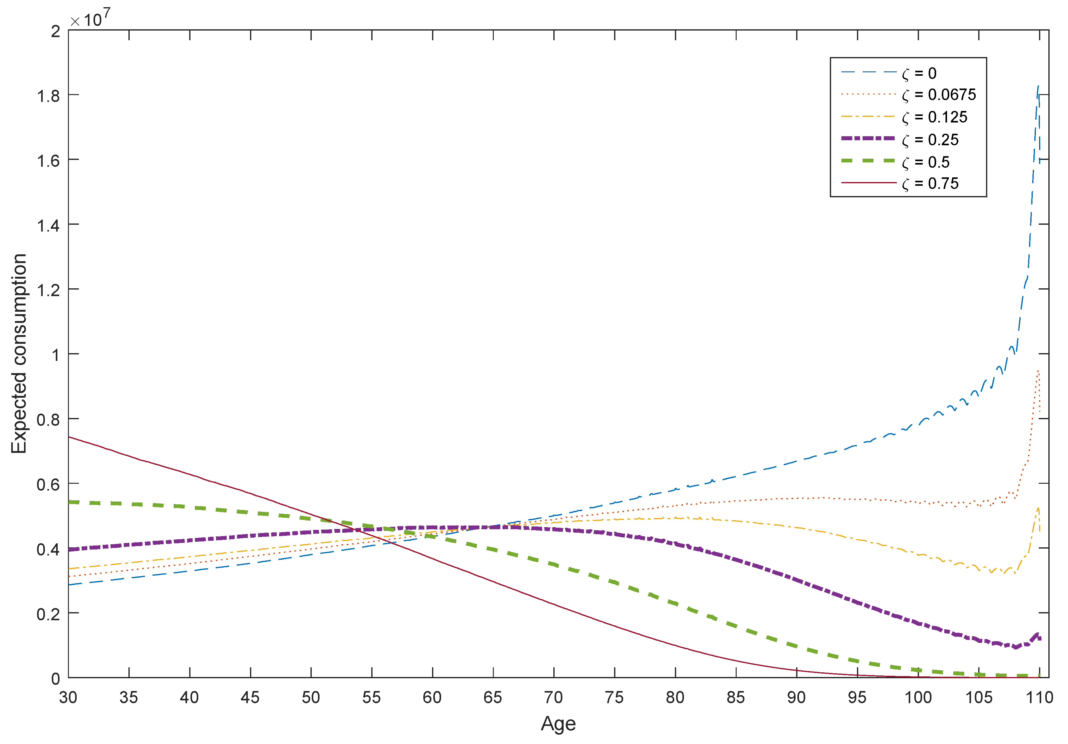
Figure 2.
Expected insurance premium for different values.
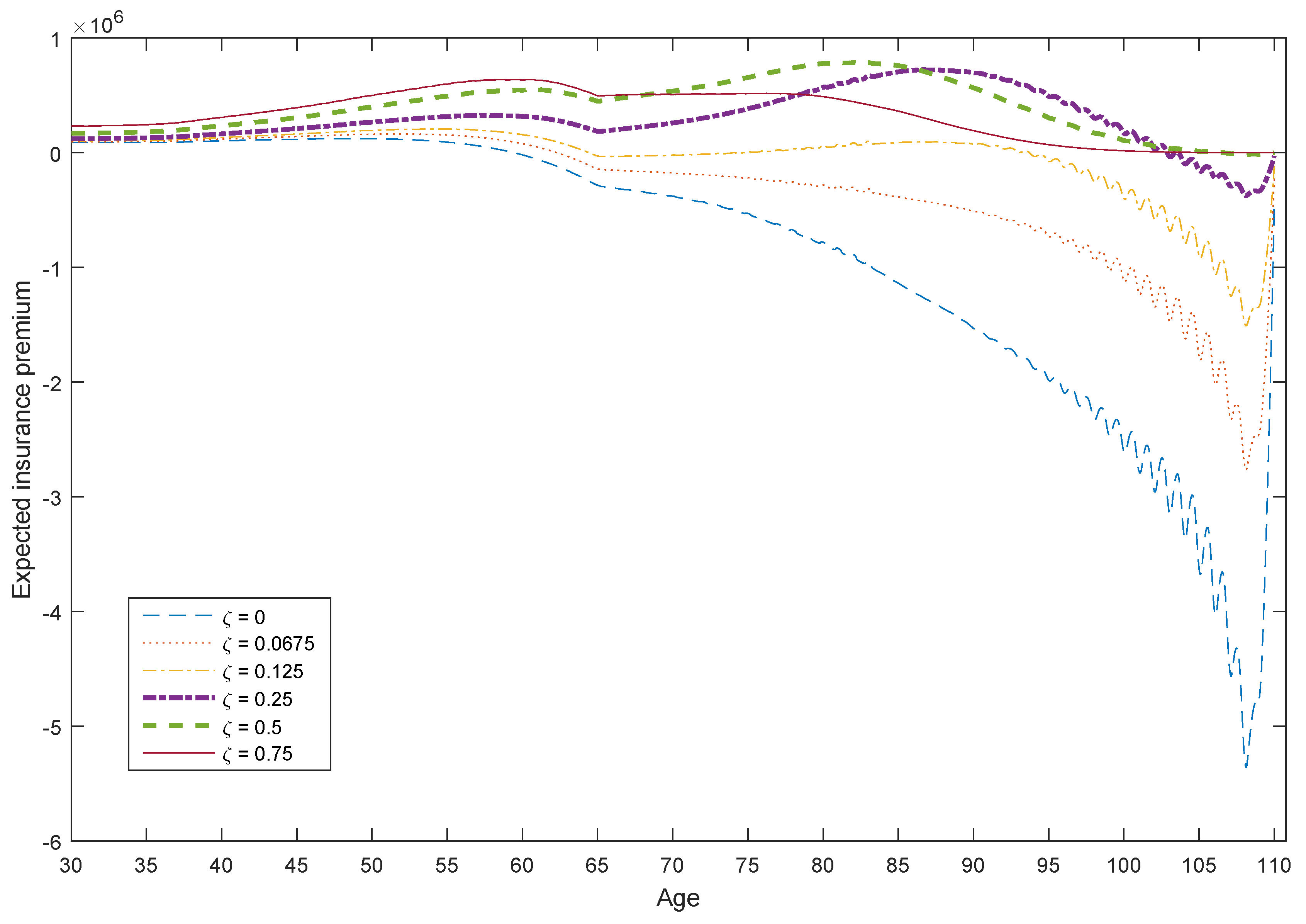
Figure 3.
Expected wealth.

Table 1.
Parameters used in the numerical simulation.
| t = 30 Y = 5,102,412 Yen | r = 0.00364 | |
© 2018 by the authors. Licensee MDPI, Basel, Switzerland. This article is an open access article distributed under the terms and conditions of the Creative Commons Attribution (CC BY) license (http://creativecommons.org/licenses/by/4.0/).
Share and Cite
MDPI and ACS Style
Tang, S.; Purcal, S.; Zhang, J. Life Insurance and Annuity Demand under Hyperbolic Discounting. Risks 2018, 6, 43. https://doi.org/10.3390/risks6020043
AMA Style
Tang S, Purcal S, Zhang J. Life Insurance and Annuity Demand under Hyperbolic Discounting. Risks. 2018; 6(2):43. https://doi.org/10.3390/risks6020043
Chicago/Turabian StyleTang, Siqi, Sachi Purcal, and Jinhui Zhang. 2018. "Life Insurance and Annuity Demand under Hyperbolic Discounting" Risks 6, no. 2: 43. https://doi.org/10.3390/risks6020043
Note that from the first issue of 2016, this journal uses article numbers instead of page numbers. See further details here.