Volatility Is Log-Normal—But Not for the Reason You Think


1
Department of Engineering & Oxford-Man Institute of Quantitative Finance, University of Oxford, Oxford OX1 3PJ, UK
2
Department of Mathematical Sciences, University of Copenhagen, 2100 København Ø, Denmark
*
Author to whom correspondence should be addressed.
Risks 2018, 6(2), 46; https://doi.org/10.3390/risks6020046
Submission received: 16 February 2018
/
Revised: 13 April 2018
/
Accepted: 18 April 2018
/
Published: 24 April 2018
Abstract
:It is impossible to discriminate between the commonly used stochastic volatility models of Heston, log-normal, and 3-over-2 on the basis of exponentially weighted averages of daily returns—even though it appears so at first sight. However, with a 5-min sampling frequency, the models can be differentiated and empirical evidence overwhelmingly favours a fast mean-reverting log-normal model.
1. Introduction: Seeing and Believing
A widespread method for measuring the instantaneous return variance1 of a price process is by an exponentially weighted average of past squared rates of returns,
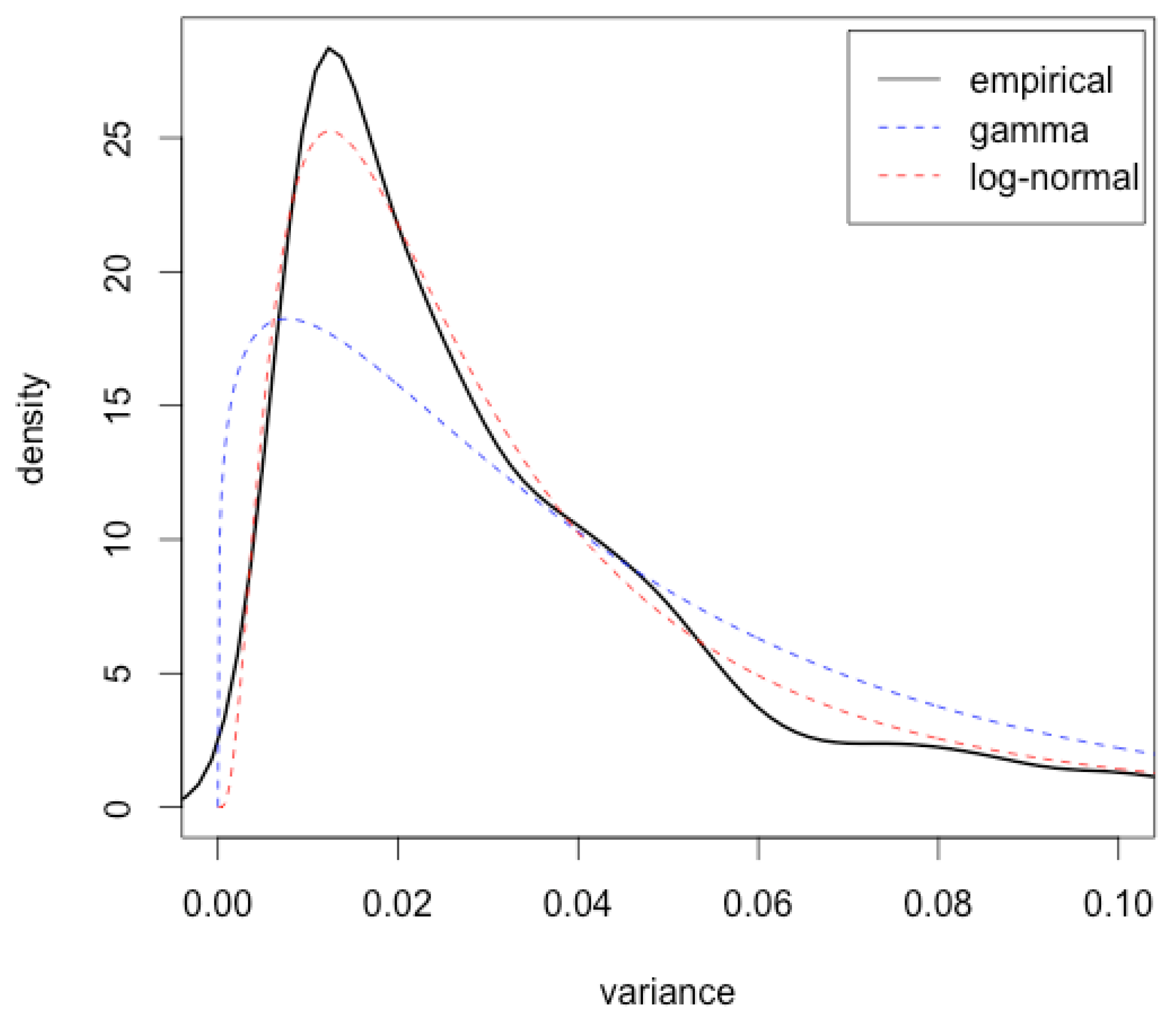
see for instance RiskMetrics (1996, Table 5.1); Wilmott (1998, Sct. 45.3); or Hull (2009, Chp. 17). We apply this measure to daily returns of the S&P500 index from January 1995 to December 2013 with the values and —as suggested by the aforementioned sources—and plot its non-parametrically estimated density in Figure 1. In the figure, we also show the best-fitting log-normal and gamma densities (i.e., densities evaluated at the respective maximum likelihood estimates). The log-normal distribution shows a decent fit, the gamma distribution does not. Ipso facto: clear empirical evidence against the Heston stochastic volatility model—whose stationary distribution is gamma—and supporting a log-normal model of volatility.
There are, however, flaws with this swift conclusion. The first appears immediately when a quantitative test is applied in place of a visual comparison. Kolmogorov-Smirnov (K-S) p-values for log-normal and gamma distances to the empirical distribution are and , respectively. Even if the log-normal distribution is closer in distance, the null hypothesis is rejected with high significance for both distributions. However, the K-S test assumes independent observations while the variance data used to estimate the density in Figure 1 is far from independent: first order auto-correlation is 0.99. This makes distributional differences look more significant than they are. Hence, the empirical density might indeed be log-normal.
Continuing that line of thought, how do we know the gamma density does not pass tests as well? The answer lies in realizing that a diffusion model makes stronger statements about the behaviour of volatility than just its stationary (unconditional, asymptotic) distribution. A diffusion model specifies conditional distributions at any time-horizon and for any initial value of volatility2. Fortunately, in the 1990s, a sound theory for statistical inference for diffusion processes was established, see Sørensen (2012) for a survey; we will draw on this theory. But we also face another problem. Equation (1) does not directly give the “true” continuous-time object that Heston and other stochastic volatility models describe. It gives a measured quantity, and as such it is contaminated by noise.
As the opening paragraph suggests, the focus of this paper is a statistical investigation of volatility models commonly used in finance. To start off, when modelling a positive quantity like variance, the log-normal distribution is a convenient choice. It is therefore not surprising that it was used for early stochastic volatility models. For a taxonomy see Table 1 in Poulsen et al. (2009). However, for option pricing the integrated variance plays a central role and its distribution is unknown in closed form for log-normal models (intuitively because the log-normal distribution is not stable under addition). No closed-form expression is therefore available for option prices. This has diminished the academic appeal as revealed by Table 1, which shows the impact (measured by a citation count) of different stochastic volatility papers. In place, option-price approximations have been suggested. The two most popular treat the opposite ends of the parametric spectrum: Hagan et al. (2002) work with the so-called SABR model where volatility has no mean-reversion, while Fouque et al. (2000) develop approximations that work well if a strong mean-reversion is present.
We investigate what we can say about volatility with statistical certainty based on volatility dynamics of observed price processes, as opposed to evidence from option prices observed from option markets. The answers are in the title. More specifically, we look at three continuous-time models (Heston, log-normal, and 3-over-2) and show that with daily measurements, Equation (1) cannot be used to discriminate between these models. Day-to-day changes are too noisy to represent the fine structure of the models, and an analysis like the one based on Figure 1 may not only be inconclusive, but outright misleading. For all models the log-normal density provides the best fit of the stationary distribution of measured variance. However, shifting to a 5-min observation frequency it is indeed possible to discriminate between the models as we show both by controlled simulation studies and with market data. We find overwhelming support for fast mean-reverting log-normal models, both for the S&P500 index and for individual stocks. We document that the log-normal model pass goodness-of-fit tests convincingly and is robust to jump corrections.
The rest of the paper is organized as follows: Section 2 reviews theory of models, inference, and measurement. Section 3 presents a comprehensive simulation study while Section 4 reports empirical results for US data. Finally, the epilogue of Section 5 discusses limitations of our analysis and where we might be heading from here.
2. Theory: Three Pieces
2.1. Continuous-Time Stochastic Volatility Models
We model the price of a given financial asset by a stochastic differential equation
where Z is a Wiener process, is the drift (rate) coefficient, and the (stochastic) instantaneous variance process is our main modelling target.
Heston (1993) suggests a model where V follows a square-root process (also known as a Feller or a Cox-Ingersoll-Ross process),
with mean reversion speed , long-term mean , diffusion , and a Wiener process W correlated to Z with coefficient . This process stays strictly positive if Feller’s condition is satisfied, i.e., . Applying the Ito formula to an integrating factor we get
From this we immediately conclude that
By taking conditional variance on Equation (4), using the Ito isometry and Equation (5) for the conditional mean, elementary integration gives
It can further be shown3 that the conditional distribution of V in Heston’s model is a non-central chi-squared distribution with degrees of freedom, non-centrality parameter , and scaling ,
If the parameters satisfy the Feller condition then V has a stationary gamma distribution with shape parameter and scale parameter 4. Arguably, our treatment of the Heston model in this paper does not fairly reflect the seminal nature of Heston’s work. He demonstrated that by working with characteristic functions (or in Fourier space), closed-form expressions could be derived for option prices up to a (numerically evaluated) integral. This transform method has since been shown to work in more general so-called affine models, see Duffie et al. (2000).
We get a log-normal model by letting , where X is a mean-reverting Gaussian process (also known as an Ornstein-Uhlenbeck, and Vasicek process)
with mean reversion speed , long-term mean , diffusion parameter , and a Wiener process W correlated with Z with correlation coefficient . Using an integrating factor and the fact that a deterministic integrand with respect to a Wiener process is normally distributed, we conclude that X is a Gaussian process (making V log-normal) with conditional distribution
and a stationary distribution which is normal with mean and variance (let ).
The dynamics of the variance in the 3-over-2 model is given by
where , and are parameters. Notice that the speed of mean-reversion depends on V itself; the drift function is quadratic, not affine. Applying the Ito formula to the reciprocal variance process ,
which implies that Y follows a square-root process with mean reversion speed and long-term mean . We will refer to the model specified by Equation (8) as the reciprocal 3-over-2 model with reciprocal parameters . This implies that V will have a stationary reciprocal gamma distribution with shape parameter5 and rate parameter .
The 3-over-2 model gives a rather “wild" behaviour of variance, which is good in some contexts. Much pricing can be done by transform methods, although from our experience almost everything requires a delicate numerical treatment. The comprehensive—and in our opinion underrated—book by Lewis (2000) treats option pricing in the 3-over-2 model. The paper by Carr and Sun (2007) renewed interest in the model,6 which was first suggested by Heston (1997) and Platen (1997). In a recent paper by Grasselli (2017), it has also been fused with Heston’s CIR process for option pricing purposes, resulting in what the author calls the 4-over-2 model.
2.2. Estimation of Discretely Observed Diffusion Processes
Suppose for now that we have observed the instantaneous variance process or some non-parameter-dependent transformation of it; generically X. The observations are taken at discrete time-points with spacings , typically one day or a few minutes for high-frequency data. We thus have an observed path of X.
For the log-normal model with parameters , the role of X is played by , and we can write the log-likelihood as
where denotes the normal density, here with (conditional) mean and variance . The maximum likelihood estimate is the argument that maximizes the log-likelihood (9). It may be found in closed form if observations are equidistant (and by a numerical optimizer if they are not). Calculating the observed information matrix
by numerical differentiation at estimated values gives an estimated standard error of the jth parameter as where denotes element of the inverse of a matrix A.
For the Heston model, the role of X is played by V itself. Optimization on the non-central chi-squared distribution that enters the Heston model’s log-likelihood is not possible in closed form, and numerically it is delicate and slow. A simple way to obtain a consistent estimator of is by plugging the conditional moments into a Gaussian likelihood and maximizing. In other words, this means using the approximate log-likelihood
where the conditional mean and variance are given by Equations (5) and (6). The reason this gives a consistent estimator is that the first order conditions for optimization of (10) are a set of so-called martingale estimating equations, see Sørensen (1999). We approximate standard errors of the estimated parameters from the observed information matrix of the approximated log-likelihood function by numerical differentiation.
In a similar fashion for the (reciprocal) 3-over-2 model, the approximate log-likelihood (10) with in place of X, can be optimized to obtain maximum likelihood estimates of the reciprocal parameters . These estimates may then be transformed to estimates of the original parameters through and while . As well, standard errors of the reciprocal parameters may be calculated from the observed information matrix and standard errors of the original parameters by the delta method.
Goodness of Fit and Uniform Residuals
A goodness-of-fit analysis that takes into consideration the full conditional structure of a diffusion process X (and not just its stationary distribution) uses so-called uniform residuals, see Pedersen (1994). With denoting the conditional distribution function of , define
The uniform residuals will be independent and identically distributed if the true distribution of X is the family , . The proof of this result, that goes back to Rosenblatt (1952), is straightforward: If the random variable X has a strictly increasing, continuous distribution function F, then is . This is combined with the Markov property and iterated expectations are used to get the independence.
For the Heston model (and the reciprocal 3-over-2 model) we use the true conditional non-central chi-squared distribution to calculate uniform residuals—not the Gaussian density used for the parameter estimation.
2.3. Measuring Volatility
Contrary to the simplifying assumption in the previous subsection, the instantaneous variance process V is not directly observable. In practice we must measure it from observations of the asset price process S. One way to do that is by Equation (1). Another way, and one that enables us to make quantitative statements about the accuracy of the measurement, comes by following Andersen and Benzoni (2009) in a study of so-called realized volatility. To this end, denote the logarithmic asset price and the continuously compounded return over a measurement interval by . Applying the Ito formula to Equation (2) and putting gives
with quadratic variation
For a partition of of the form , the realized variance is defined by
and general semimartingale theory ensures convergence in probability7
For high-frequency returns (a large n) gives a good approximation of and we may use for some to obtain a measured variance path. Thus, to adopt our notation, for an asset log-price Y observed at time points and a measurement interval (say one day), i.e., an observation frequency set by n (say 5 minutes), calculate
for as the measured variance path of the non-observable variance . Note that we obtain daily variance measurements while we require asset price observations of a much higher frequency. Of course, we may reduce n to get more frequent variance measurements but for a cost of poorer approximation with respect to the convergence in (12).
We have described a simple-to-implement, model independent, and theoretically sound measure for realized and instantaneous variance. However, it is far from the only method. For instance, Reno (2008) describes the use of so-called -sequences and kernels for volatility measurement while Andreasen (2016, Equation (2), p. 29) suggests an estimator based on absolute, not squared, returns. A different, global time-series approach is offered by the numerous variants of GARCH models, see Engle et al. (2012). We refrain from analyzing these techniques further. Partly in the interest of space, partly because specific estimation choices might stack the deck for or against one of our three models.
From a theoretical point of view, Equation (12) tells us that the higher our sampling frequency is, the more accurately we measure quadratic variation by summing squared increments. However, high-frequency data are not just a blessing, they come with perils in the form of market microstructure effects. To illustrate, suppose the observed log-price is contaminated by (white) noise, , where all ’s are independent and, say, . In this case an expression like (13) would contain a term of the form
that clearly diverges as . This means that if we use Equation (13) naively, there is an optimal observation frequency. Where that optimal frequency lies depends on the shape and magnitude of the market microstructure noise (which varies from market to market). Consensus in the literature says that it is less than 5 minutes (which is generally considered free from noise) but more than 1 second. However, in the case of noise and high frequencies we can do better than Equation (13). By a careful treatment of double asymptotics, Christensen et al. (2014) prove that with clever local smoothing (so-called pre-averaging) it is possible to remove market microstructure effects (like the white noise above, but also bid-ask bounce and outright outliers) without compromising too much of the measurement quality of volatility and of jumps; the latter of which we will consider below.
Realized Volatility for an Asset Price with Jumps
The asset price process in Equation (2) has continuous paths, arguably a restrictive constraint for market data of asset prices8. To this end, Andersen and Benzoni (2009) suggest adding a compound Poisson-type, finite activity jump-part to the price dynamics,
where is a Poisson process uncorrelated to Z, while determines the magnitude of a jump that occurs at time t. The Ito formula for diffusions with jumps applied to gives
The jump term is non-zero only if a jump occurs at time t and it should be understood in integral form
where are the random jump times of N in . The quadratic variation of Y in (14) includes both the integrated variance and a jump part
while the convergence
still holds. As an estimator for the integrated variance part, we employ the realized bipower variation introduced by Barndorff-Nielsen and Shephard (2004)
which provides a consistent estimate of the variance which is robust to jumps9. The ratio gives a measure of how much of the cumulative variance is due to jumps.
3. Simulation: Model Discrimination
To asses the statistical properties of our model discrimination test, we look at simulated asset price and variance data.
The first port of call when simulating solutions to stochastic differential equations is the Euler scheme, see Kloeden and Platen (1992). It provides a simple method for the generation of time-discrete approximations to sample paths. However, we quickly run into problems with the Euler scheme for the models we consider as it may produce negative variances. Therefore, we require methods that better preserve distributional properties, positivity specifically. For the log-normal model the solution is straightforward: simulate the log of the process; this is easy to do in an exact manner. Alas, the log-trick does not work for the Heston model; apply the Ito formula to see why. Therefore, we use the simulation scheme from Broadie and Kaya (2006) with a modification that approximates the integrated variance with a trapezoidal rule, see Platen and Bruti-Liberati (2010). This scheme is (almost) exact, but slow. Faster methods have been suggested, see Andersen et al. (2010). These generally preserve positivity but not exact distributional characteristics. In a similar fashion, Baldeaux (2012) provides an exact simulation method for the 3-over-2 model.
S&P 500 Data Revisited
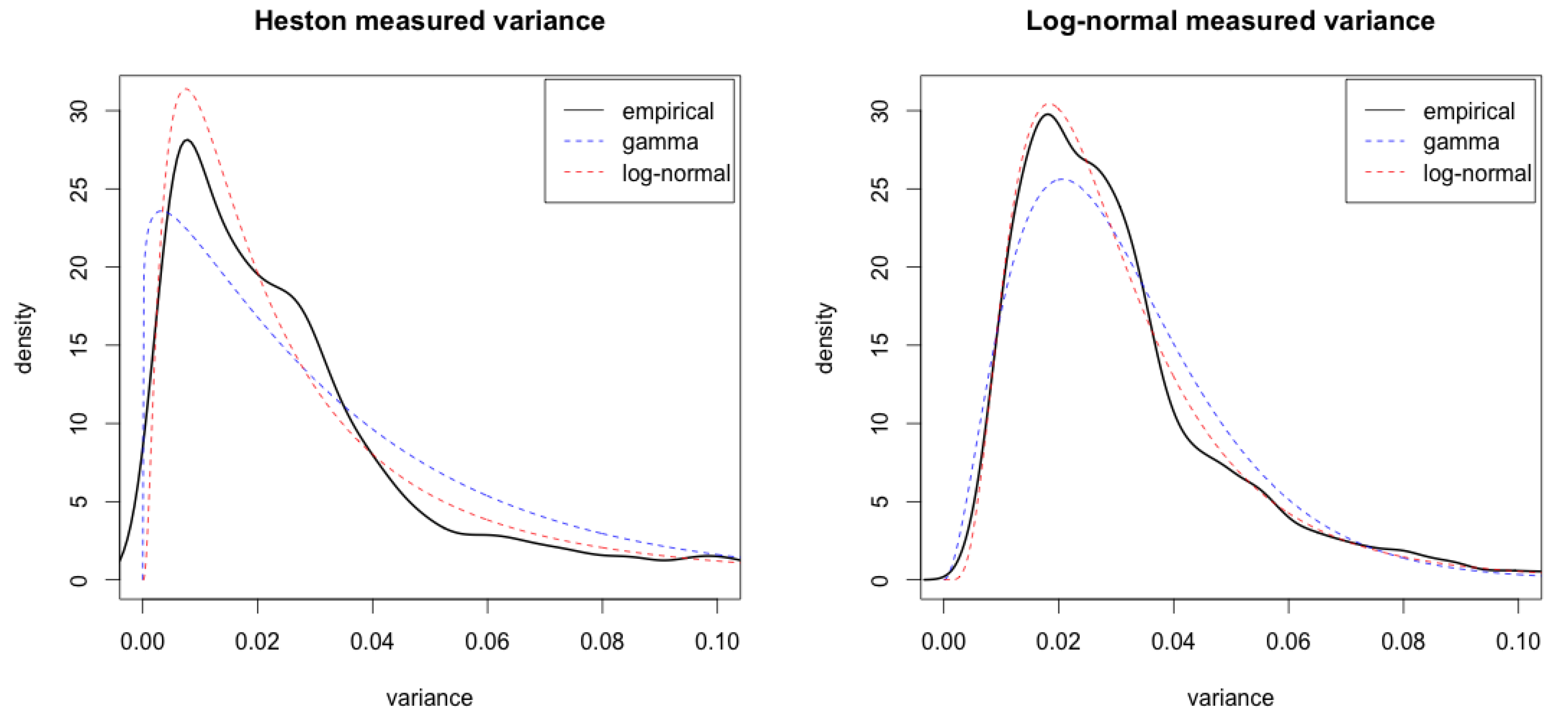
To return to the question of credibility in the analysis of the introduction, we perform a mimicking simulation experiment. We apply the exponentially weighted moving average of Equation (1) to 4532 daily prices simulated from either Heston or the log-normal model with parameters given by the S & P 500 estimates in Section 4. The result for measured variance from Heston’s model shows that fitting unconditional distributions leads to the the same conclusion as with the S&P 500 data: the data appears to be log-normal—see the left-hand graph in Figure 2.10
To overcome the correlation problem and to fully exploit conditional information, we run a discriminatory test between the three models based on uniform residuals when variance is measured by Equation (1). The results are listed in the right-most column of Table 2, where we report the p-values from a chi-squared test under the null-hypothesis that residuals are uniform.For every simulation, the true underlying model is rejected with high significance—as are the wrong models. Variance measured by Equation (1) is simply too noisy to capture the fine structure properties implied by continuous-time stochastic volatility models.
Next, we simulate returns with a 5-min frequency with ,11 i.e., a two-day aggregation, for the measurement of instantaneous variance. We choose to use of a 5-min frequency for several reasons (or, if you like, for a compromise): (i) it is common in the literature; (ii) data is available for a large range of markets from plain vanilla (although not open source) academic databases; (iii) our experiments show that model separation is possible; and (iv) we avoid contamination from market microstructure noise12. We then apply Equation (13) and run the uniform residuals goodness-of-fit test on this data. This gives the results reported in the second-to-right column of Table 2. Here we achieve model discrimination. In all three cases (across models and simulations), false models are rejected while the true model is accepted. We also apply the goodness-of-fit analysis on the simulated variance itself. In this way we investigate if there is any gain in going beyond a 5-min. sampling frequency. The results in the second-to-left column in Table 2 show that there isn’t. Finally, we run 1000 repetitions for each of the above test cases and record p-values across all test alternatives. The results are consistent with Table 2: for close to all repetitions (∼99–100%) we achieve model discrimination based on the 5-min realized volatility, while the exponentially moving average rejects all models, in all cases.
4. Empirics: Horseraces between Models
The empirical analysis is based on data from the S&P 500 index (or, to be precise, an exchange traded fund (ETF) that tracks the S&P 500 index) and ten arbitrarily chosen securities listed on the New York Stock Exchange (NYSE). Their ticker symbols and corresponding number of observations are given in Table 4. All data is retrieved from the TAQ database via Wharton Research Data Services. The raw data consists of intraday tick-by-tick trade data. This data is, however, not directly suited for analysis and we apply a series of preprocessing methods. Specifically, we use the step-by-step cleaning procedure proposed by Barndorff-Nielsen et al. (2009). First, entries with zero prices are deleted, as are entries with an abnormal sale condition indicated from the code of the trade. The data is then restricted to include trades only from the exchange where the security is listed. Entries with the same time stamp are replaced by the median price in the last step.
The cleaned data will be on an irregular tick-by-tick time scale. We aggregates prices to an equidistant 5-min time grid by taking the last realized price before each grid point. Finally, the data is restricted to exchange trading hours 9:30 a.m. to 4:00 p.m. from Monday to Friday.
The realized volatility measure is applied with a resolution of prices per variance measurement for the first step of the test methodology and a plot of the resulting variance path of 1920 observations is shown in the right-hand graph of Figure 3. The measured variance is used in the second step for the maximum (approximate) likelihood estimation where a numerical optimization is performed on the likelihood function for each model. Resulting estimated parameters and standard errors are reported in Table 3. Note that even though each of the parameters has the same qualitative interpretation across models ( mean level, speed of mean-reversion, volatility of volatility), their numerical values cannot be compared directly.
As a sanity check, let us take a look at typical levels of instantaneous volatility that are implied by estimated parameters. For the Heston model it is and for the log-normal model it is —both in line with what we would anticipate. However, we have to be careful here as non-linear functions and parameters are in a range where Jensen’s inequality matters. For instance, in the log-normal model, the stationary distribution for has a mean . The 3-over-2 parameter estimates look strange at first sight, but we can think of them this way. From Equation (8) the reciprocal parameters are . From the right-hand panel of Figure 3 we see that 119 is a typical value for reciprocal variance, and that this process covers a large range of values leading to combined high volatility and high speed of mean-reversion. The morale is that a non-linear and ill-fitting (see the right-most panel in Figure 4) model is hard to interpret.
To get a quantitative feeling for the speed of mean-reversion parameters, we use that for a process with linear mean-reversion, the time it takes to halve the deviation in expectation between current level and long-term level is
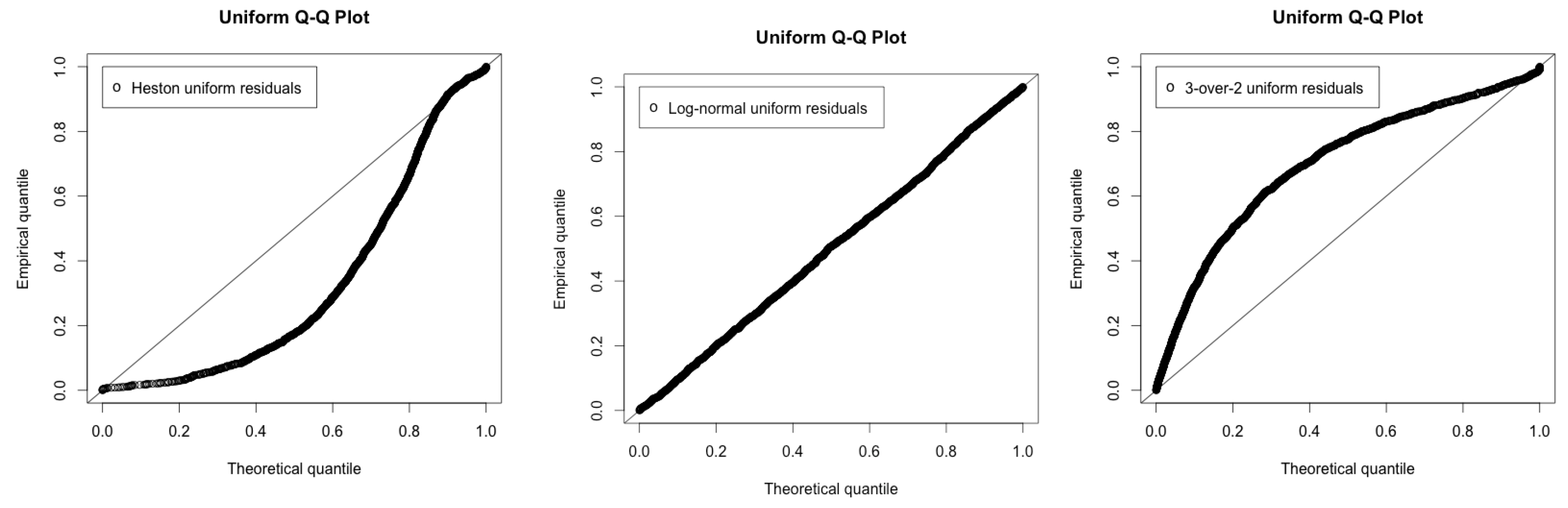
The estimates imply that for Heston model the half-life of deviances is about eight days, for the log-normal model the half-life (for log-variance) is just over three days. This is strong mean-reversion. Or differently put, mean-reversion is in effect over short time-scales. For interest rate models, typical -values are 0.1–0.25 which implies deviance half-life of 3–7 years. Such strong mean-reversion plays havoc with our usual “quantitative intuitive interpretation”, where it determines the standard deviation of the change (in absolute or relative terms) of the process over one year, i.e., a change of ± the volatility is “nothing out of the ordinary”. That interpretation is non-sensical here. If applied it would tell us that the instantaneous variance in Heston is typically in the range , and that volatilities of 5000% and 0.05% are imminently plausible in the log-normal model. It is the combination of high speed of mean-reversion and high volatility of volatility that is needed to generate the decidedly spiky behaviour of volatility which is what our likelihood approach aims at capturing, For the Heston model we have , so the Feller condition is violated by a factor 10. However, what we think is the most striking result in Table 3 is the last column, which contains goodness-of-fit tests for the different models: p-values for Kolmogorov-Smirnov on the uniform residuals. The log-normal model provides a (surprisingly) good fit (), Heston and 3-over-2 do not (; the quantile plots in Figure 4 gives further visual evidence.
Comparing our findings to the literature, our most clear ally in the recent empirical literature is Christoffersen et al. (2010) who also find strong support for log-normal(’ish) volatility models compared to Heston and 3-over-2. They only use daily data, so their parameter values (see Table 1 in Christoffersen et al. (2010)) do not pick up the fast mean-reverting feature. In that respect, our results are most in line with Fouque et al. (2000) who use a log-normal model (without explicit discriminatory goodness-of-fit test) and document strong mean-reversion (even stronger than ours; 200–250—although other work by the same authors suggests ). Similarly to us Andersen et al. (2001) (Figures 1–3 for instance) report log-normality of variance measured on 5-min sampling. They do not find fast mean-reversion, but rather that volatility has long-term memory.

Table 4.
The number of asset price and measured variance observations for the stock data.
| # obs | IBM | MCD | CAT | MMM | MCO | XOM | AZN | GS | HPQ | FDX |
|---|---|---|---|---|---|---|---|---|---|---|
| price | 246,308 | 328,111 | 328,107 | 328,108 | 271,580 | 288,846 | 302,350 | 300,759 | 239,356 | 328,104 |
| variance | 1282 | 1708 | 1708 | 1708 | 1414 | 1504 | 1574 | 1566 | 1246 | 1708 |
4.1. Individual Stocks
A sceptic might say: “The log-normality of the index is an aggregation effect: some stocks are Heston, some are 3-over-2, and when you mix them all up, it comes out as log-normal”. However, it is not, as results summarised in Table 5 show. Heston and the 3-over-2 models are rejected with all p-values indistinguishable from 0, the log-normal model is accepted for all 10 stocks (although 2 are borderline), mean-reversion is strong (all ’s > 50), and volatility of volatility is correspondingly high in order to generate spikes.
4.2. Jump Corrections
The sceptic might continue: “When you use Equation (13) you pick up both jumps and diffusive volatility. It think it’s the jumps that cause log-normality. For the diffusive part Heston will do”. (Conveniently, options can be priced using transform methods from Duffie et al. (2000).) Table 6 shows that log-normality of variance prevails when it is measured through bipower variation.
5. Conclusions and Future Work
In this paper we have demonstrated that log-normal models provide a significantly better description of the empirical behaviour of instantaneous variance than the Heston and the 3-over-2 models. However, at coarser time-resolutions it can be hard to discriminate between the models. Our intention has been to give a reasonably self-contained treatment of the theory and used models and methods, rather than to facilitate a replication of the results13.
We find that to replicate the spiky but stationary behaviour of volatility, we need a combination of strong mean-reversion and high volatility of volatility. From a modelling perspective this suggests that we look beyond the diffusive model, towards models with higher degree of path roughness (as measured by degree of Hölder continuity) of volatility. A promising line of research are the rough volatility models suggested in Gatheral et al. (2018) (see also Andreasen (2017)) where volatility is driven by a fractional Brownian motion.
Finally, it must be mentioned that the strongly mean-reverting volatility diffusion models that we investigate go against an often-documented (see the discussion in Bennedsen et al. (2017)) empirical property of volatility: long memory (persistence) at low frequencies. A natural solution (LeBaron (2001), Fouque et al. (2003)) in the realm of diffusions is to model instantaneous volatility as a sum of component process with vastly differing speeds of mean-reversion. It is less obvious how to do this in a fractional setting (where path roughness and persistence are exact opposites), but Bennedsen et al. (2017) suggest the use of semistationary processes. To us, the big question in this context is: What matters where? For which problems is the high frequency important, for which is the low frequency important? Are there problems with mixed effects? Our hunch is high frequency for option pricing and low frequency for portfolio choice, but we are yet to see quantitative evidence for this—although Bollerslev et al. (2018) is a promising framework for investigations.
Author Contributions
Martin Tegnér and Rolf Poulsen conceived and designed the experiments and wrote the paper; Martin Tegnér did the programming and performed the computational and end empirical experiments.
Acknowledgments
The authors gratefully acknowledge support from the Danish Strategic Research Council, Program Committee for Strategic Growth Technologies, via the research center HIPERFIT: Functional High Performance Computing for Financial Information Technology (hipert.dk) under contract number 10-092299.
Conflicts of Interest
The authors declare no conflict of interest.
References
- Andersen, Leif B. G., Peter Jäckel, and Christian Kahl. 2010. Simulation of square-root processes. In Encyclopedia of Quantitative Finance. Edited by Rama Cont. Hoboken: Wiley, pp. 1642–49. [Google Scholar]
- Andersen, Torben Gustav, and Luca Benzoni. 2009. Realized volatility. In Handbook of Financial Time Series. Edited by Torben Gustav Andersen, Richard A. Davis, Jens-Peter Kreiß and Thomas V. Mikosch. Berlin: Springer, pp. 555–75. [Google Scholar]
- Andersen, Torben G., Tim Bollerslev, Francis X. Diebold, and Keiko Ebens. 2001. The distribution of realized stock return volatility. Journal of Financial Economics 61: 43–76. [Google Scholar] [CrossRef]
- Andreasen, Jesper. 2016. Time series estimation of stochastic models. Paper presented at Global Derivatives, Budapest, Hungray, 11 May 2016. [Google Scholar]
- Andreasen, Jesper. 2017. Tough volatility. Presentation at Danske Markets, Copenhagen, Denmark, 12 December 2017; Available online: https://tinyurl.com/ycjfoe6d (accessed on 1 February 2018).
- Baldeaux, Jan. 2012. Exact simulation of the 3/2 model. International Journal of Theoretical and Applied Finance 15: 1250032. [Google Scholar] [CrossRef]
- Barndorff-Nielsen, Ole E., P. Reinhard Hansen, Asger Lunde, and Neil Shephard. 2009. Realized kernels in practice: Trades and quotes. Econometrics Journal 12: C1–C32. [Google Scholar] [CrossRef]
- Barndorff-Nielsen, Ole E., and Neil Shephard. 2004. Power and bipower variation with stochastic volatility and jumps. Journal of Financial Econometrics 2: 1–37. [Google Scholar] [CrossRef]
- Bennedsen, Mikkel, Asger Lunde, and Mikko S. Pakkanen. 2017. Decoupling the short- and long-term beviour of stochastic volatility. arXiv, arXiv:1610.00332. [Google Scholar]
- Bollerslev, Tim, John Hood Benjamin abd Huss, and Lasse Heje Pedersen. 2018. Risk everywhere: Modeling and managing volatility. In Review of Financial Studies. forthcoming. [Google Scholar]
- Broadie, Mark, and Özgür Kaya. 2006. Exact simulation of stochastic volatility and other affine jump diffusion processes. Operations Research 54: 217–31. [Google Scholar] [CrossRef]
- Cairns, Andrew J. G. 2004. Intereast Rate Models: an Introduction. Princeton: Princeton University Press. [Google Scholar]
- Carr, Peter, and Jian Sun. 2007. A new approach for option pricing under stochastic volatility. Review of Derivatives Research 10: 87–150. [Google Scholar] [CrossRef]
- Chan, Kalok C., G. Andrew Karolyi, Francis A. Longstaff, and Anthony B. Sanders. 1992. An empirical comparison of alternative models of the short term interest rate. Journal of Finance 47: 1209–27. [Google Scholar] [CrossRef]
- Christensen, Kim, Roel C. A. Oomen, and Mark Podolskij. 2014. Fact or friction: Jumps at ultra high frequency. Journal of Financial Economics 114: 576–99. [Google Scholar] [CrossRef]
- Christoffersen, P., K. Jacobs, and K. Mimouni. 2010. Models for s&p 500 dynamics: Evidence from realized volatility, daily returns and options prices. Review of Financial Studies 23: 3141–89. [Google Scholar]
- Duffie, Darrell, Jun Pan, and Kenneth Singleton. 2000. Transform analysis and asset pricing for affine jump-diffusions. Econometrica 68: 1343–76. [Google Scholar] [CrossRef]
- Engle, Robert F., Sergio M. Focardi, and Frank J. Fabozzi. 2012. Arch/garch models in applied financial econometrics. In Encyclopedia of Financial Models. Hoboken: Wiley. [Google Scholar]
- Fouque, Jean-Pierre, George Papanicolaou, and K. Ronnie Sircar. 2000. Mean-reverting stochastic volatility. International Journal of Theoretical and Applied Finance 3: 101–42. [Google Scholar] [CrossRef]
- Fouque, Jean-Pierre, George Papanicolaou, Ronnie Sircar, and Knut Solna. 2003. Multiscale stochastic volatility asymptotics. SIAM J. Multiscale Modeling and Simulation 2: 22–42. [Google Scholar] [CrossRef]
- Gatheral, Jim, Thibault Jaisson, and Mathieu Rosenbaum. 2014. Volatility is rough. Quantitative Finance. forthcoming. [Google Scholar] [CrossRef]
- Grasselli, Martino. 2017. The 4/2 stochastic volatility model: a unified approach for the Heston and the 3/2 model. Mathematical Finance 27: 1013–1034. [Google Scholar] [CrossRef]
- Hagan, Patrick S., Deep Kumar, Andrew S. Lesniewski, and Diana E. Woodward. 2002. Managing smile risk. Wilmott Magazine, July. 84–108. [Google Scholar]
- Heston, Steven L. 1993. A closed-form solution for options with stochastic volatility with applications to bond and currency options. Review of Financial Studies 6: 327–43. [Google Scholar] [CrossRef]
- Heston, Steven L. 1997. A Simple nEw Formula for Options with Stochastic Volatility. Technical report. St. Louis: Washington University of St. Louis. [Google Scholar]
- Hull, John C. 2009. Options, Futures and Other Derivatives. Delhi: Pearson/Prentice Hall. [Google Scholar]
- Jönsson, Martin. 2016. Essays on Quantitative Finance. Ph. D. thesis, University of Copenhagen, København, Denmark. [Google Scholar]
- Kloeden, Peter E., and Eckhard Platen. 1992. Numerical Solution of Stochastic Differential Equations. Berlin: Springer. [Google Scholar]
- LeBaron, Blake. 2001. Stochastic volatility as a simple generator of apparent financial power laws and long memory. Quantitative Finance 1: 621–31. [Google Scholar] [CrossRef]
- Lewis, Alan L. 2000. Option Valuation under Stochastic Volatility. Newport Beach: Finance Press. [Google Scholar]
- Pedersen, Asger Roer. 1994. Uniform Residuals for Discretely Observed Diffusion Processes. Technical Report, Research Report No. 295. Aarhus: University of Aarhus. [Google Scholar]
- Platen, Eckhard, and Nicola Bruti-Liberati. 2010. Numerical Solution of Stochastic Differential Equations with Jumps in Finance. Berlin: Springer, vol. 64. [Google Scholar]
- Platen, Eckhard. 1997. A Non-Linear Stochastic Volatility Model. Financial Mathematics Research Report No. FMRR 005-97. Canberra: Center for Financial Mathematics, Australian National University. [Google Scholar]
- Poulsen, Rolf, Klaus Reiner Schenk-Hoppé, and Christian-Oliver Ewald. 2009. Risk minimization in stochastic volatility models: Model risk and empirical performance. Quantitative Finance 9: 693–704. [Google Scholar] [CrossRef]
- Reno, Roberto. 2008. Nonparametric estimation of the diffusion coefficient of stochastic volatility models. Econometric Theory 24: 1174–206. [Google Scholar] [CrossRef]
- RiskMetrics. 1996. Riskmetrics—Technical Document. Technical Report. London: JP Morgan/Reuters, Available online: https://www.msci.com/documents/10199/5915b101-4206-4ba0-aee2-3449d5c7e95a (accessed on 1 April 2016).
- Rosenblatt, Murray. 1952. Remarks on a multivariate transformation. Annals of Mathematical Statistics 23: 470–72. [Google Scholar] [CrossRef]
- Sørensen, Michael. 1999. On the asymptotics of estimating functions. Brazilian Journal of Probability and Statistics 13: 111–36. [Google Scholar]
- Sørensen, Michael. 2012. Statistical methods for stochastic differential equations. In Estimating Functions for Diffusion-Type Processes. Boca Raton: CRC Press, pp. 1–107. [Google Scholar]
- Wilmott, Paul. 1998. Derivatives. Hoboken: Wiley. [Google Scholar]
| 1. | Often, we will use the term (instantaneous) volatility. This means taking the square root of the instantaneous variance and annualizing by a multiplying factor , where 252 represents the (approximate) number of trading days in a year. The annualization is a convention, not a theorem; when returns are not iid—which is the case for mean-reverting stochastic volatility models—we do not get the standard deviation of yearly returns by multiplying with . Notice further that log-normal models are stable to roots and squares: it is not misleading to say “volatility is log-normal” even though we model variance. The Heston and the 3-over-2 models do not posses this stability. |
| 2. | A further complication is that for the models we consider, not all parameters are identifiable by their stationary distribution. |
| 3. | A detailed derivation of this is in Cairns (2004, Appendix B.2). |
| 4. | Notice that stationary distribution depends on and only through . This was what we meant when we talked about identification problems in an earlier footnote. |
| 5. | The first moment of the inverse-gamma distribution is defined if the shape parameter is greater than one, a condition certified by the Feller condition. In this case . |
| 6. | Older readers may remember that Chan et al. (1992), a very influential paper in the 90’ies, estimated the volatility of the short-term interest rate, r to be of the form , i.e., almost exactly 3/2, but their model had an affine drift, which (7) doesn’t. |
| 7. | The convergence holds for any partition whose mesh size goes to 0. |
| 8. | Although, as Christensen et al. (2014) points out, perhaps not as restrictive as believed in some areas in the literature. |
| 9. | The presence of the -factor indicates that this is not as obvious as it might seem. |
| 10. | We have been trying to find at least a heuristic explanation for this small (or coarse) sample log-normality, but have not managed to come up with anything particularly convincing. |
| 11. | The two-day aggregation of 5-min returns may seem like a strange choice; one-day aggregation is common in the literature and appears the natural choice. However, our experiments (not reported here but see Jönsson (2016) for more details) show that one-day aggregation of 5-min returns diminishes model separation power: lower noise is indeed worth an increased bias. |
| 12. | Quantitative evidence: In https://tinyurl.com/y9epg6a7 we simulate a log-normal volatility model with the parameters from Table 3 in this paper at 5-min intervals and add market microstructure noise using the parameter specification in Table 2 in Christensen et al. (2014). We find that the average absolute deviation between true volatility and volatility measured by noise-free realized variance is about 75 times higher than the average absolute difference between realized variances with and without noise. |
| 13. | We are not allowed to make the high-frequency data public. |
Figure 1.
Estimated empirical density of the annualized measured instantaneous S&P500 variance (4552 daily observations 1996–2013 using Equation (1)) together with fitted log-normal and gamma densities.
Figure 1.
Estimated empirical density of the annualized measured instantaneous S&P500 variance (4552 daily observations 1996–2013 using Equation (1)) together with fitted log-normal and gamma densities.

Figure 2.
Fitted empirical, log-normal and gamma densities to measured variance with of 4532 simulated prices with Heston’s (left figure) and the log-normal model (right figure).
Figure 2.
Fitted empirical, log-normal and gamma densities to measured variance with of 4532 simulated prices with Heston’s (left figure) and the log-normal model (right figure).

Figure 3.
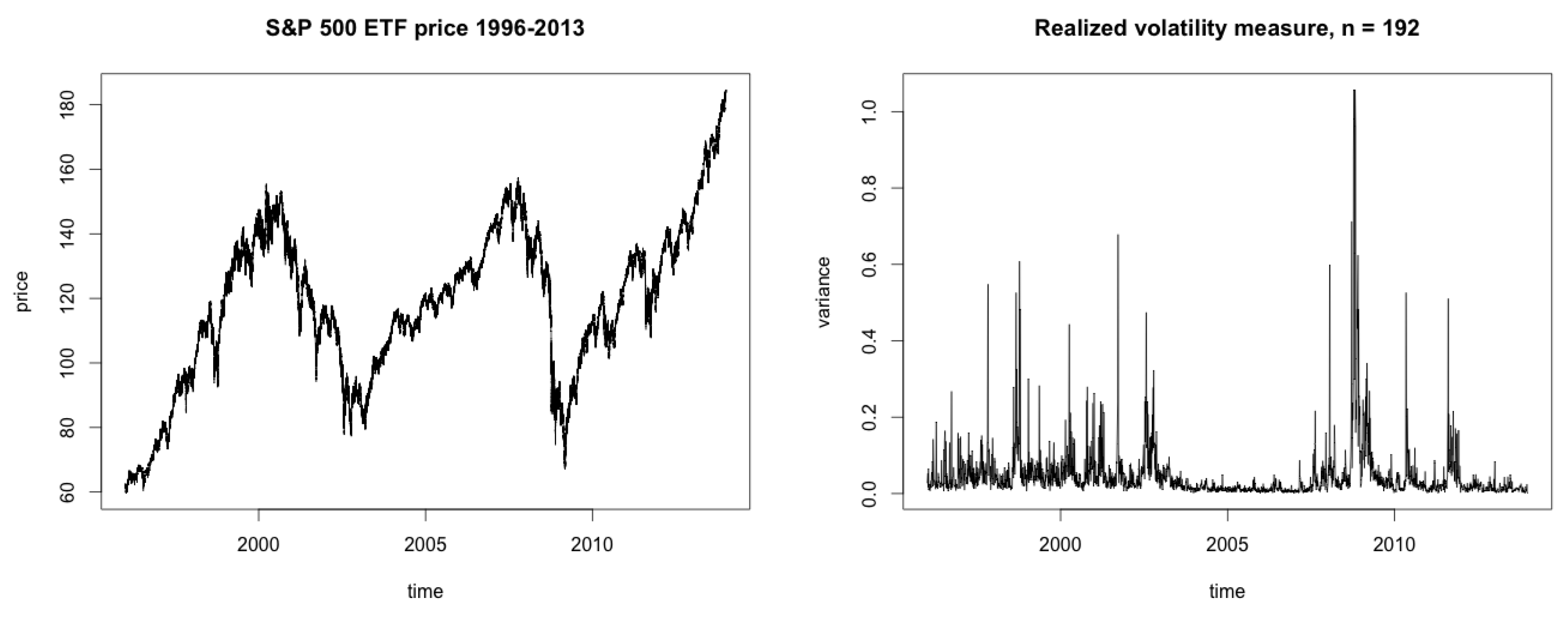
The left figure shows the S&P 500 ETF price from 2 January 1996 to 31 December 2013 with a 5-min. frequency and a total of 368,724 observations. Right figure: variance of the S&P 500 ETF price measured by realized volatility with frequency and a total of 1920 observations.
Figure 3.
The left figure shows the S&P 500 ETF price from 2 January 1996 to 31 December 2013 with a 5-min. frequency and a total of 368,724 observations. Right figure: variance of the S&P 500 ETF price measured by realized volatility with frequency and a total of 1920 observations.

Figure 4.
Quantile plots of the uniform distribution from uniform residuals calculated with measured S&P 500 variance.
Figure 4.
Quantile plots of the uniform distribution from uniform residuals calculated with measured S&P 500 variance.

Table 1.
Impact of stochastic volatility research measured by citations in Google Scholar on 15 February 2018.
Table 1.
Impact of stochastic volatility research measured by citations in Google Scholar on 15 February 2018.
| Model Type | Source | # Citations (Yearly Rate) |
|---|---|---|
| Affine, basic | Heston (1993) | 7637 (310) |
| Affine, fancy | Duffie et al. (2000) | 3009 (171) |
| Log-normal, no mean-reversion | Hagan et al. (2002) | 974 (62) |
| Log-normal, fast mean-reversion | Fouque et al. (2000) | 175 (10) |
| 3-over-2 | Carr and Sun (2007) | 94 (9) |
| All of the above | Lewis (2000) | 766 (43) |
Table 2.
Discriminatory power of Kolmogorov-Smirnov tests on uniform residuals for different methods of variance measurement: p-values from the chi-square test under the hypothesis indicated in the test alternative column.
Table 2.
Discriminatory power of Kolmogorov-Smirnov tests on uniform residuals for different methods of variance measurement: p-values from the chi-square test under the hypothesis indicated in the test alternative column.
| True Model: Heston | Variance Measurement | ||
|---|---|---|---|
| Test alternative | true simulated | 2-day, 5-min. realized | Equation (1) |
| Heston | 0.79 | 0.57 | 0 |
| log-normal | 0 | 0 | 0 |
| 3-over-2 | 0 | 0 | 0 |
| True model: Log-normal | Variance measurement | ||
| Test alternative | true simulated | 2-day, 5-min. realized | Equation (1) |
| Heston | 0 | 0 | 0 |
| log-normal | 0.72 | 0.78 | 0 |
| 3-over-2 | 0 | 0 | 0 |
| True model: 3-over-2 | Variance measurement | ||
| Test alternative | true simulated | 2-day, 5-min. realized | Equation (1) |
| Heston | 0 | 0 | 0 |
| log-normal | 0 | 0 | 0 |
| 3-over-2 | 0.26 | 0.90 | 0 |
Table 3.
S&P 500: Estimated parameters and standard errors from (approximate) maximum likelihood estimation of the Heston, log-normal, and 3-over-2 models.
Table 3.
S&P 500: Estimated parameters and standard errors from (approximate) maximum likelihood estimation of the Heston, log-normal, and 3-over-2 models.
| K-S p-Value | ||||
|---|---|---|---|---|
| Heston | 21.7 (3.63) | 0.022 (0.0049) | 2.98 (0.08) | 0.00 |
| log-normal | 56.1 (3.36) | −3.65 (0.049) | 11.5 (0.24) | 0.68 |
| 3-over-2 | 2.7 (5.64) | 30.0 (62.7) | 98.2 (2.0) | 0.00 |
Table 5.
Maximum likelihood estimated parameters and standard errors from the realized volatility measured variance with .
Table 5.
Maximum likelihood estimated parameters and standard errors from the realized volatility measured variance with .
| Heston | IBM | MCD | CAT | MMM | MCO | XOM | AZN | GS | HPQ | FDX |
|---|---|---|---|---|---|---|---|---|---|---|
| 75.1 (7.2) | 18.2 (4.0) | 71.6 (5.3) | 37.0 (4.52) | 100.0 (6.85) | 45.4 (4.55) | 113.0 (7.92) | 41.6 (5.14) | 116.9 (12.1) | 65.2 (6.79) | |
| 0.024 (0.004) | 0.052 (0.012) | 0.112 (0.009) | 0.061 (0.006) | 0.096 (0.009) | 0.052 (0.005) | 0.069 (0.005) | 0.027 (0.009) | 0.14 (0.012) | 0.082 (0.008) | |
| 6.89 (0.4) | 4.14 (0.1) | 7.21 (0.2) | 3.89 (0.1) | 10.1 (0.4) | 3.61 (0.1) | 7.76 (0.3) | 7.97 (0.3) | 12.6 (0.6) | 6.62 (0.2) | |
| K/S p-value | 0.00 | 0.00 | 0.00 | 0.00 | 0.00 | 0.00 | 0.00 | 0.00 | 0.00 | 0.00 |
| Lognormal | ||||||||||
| 86.6 (6.0) | 61.1 (3.8) | 83.9 (5.1) | 76.9 (4.7) | 71.6 (4.8) | 72.3 (4.7) | 126.2 (8.6) | 58.3 (3.8) | 102.2 (7.4) | 88.0 (5.4) | |
| −3.31 (0.05) | −2.96 (0.05) | −2.45 (0.04) | −3.08 (0.04) | −2.60 (0.05) | −3.10 (0.04) | −2.97 (0.04) | −2.49 (0.05) | −2.54 (0.05) | −2.63 (0.04) | |
| 13.5 (0.4) | 11.4 (0.3) | 12.7 (0.3) | 12.1 (0.3) | 43.8 (0.3) | 11.3 (0.3) | 16.6 (0.5) | 11.6 (0.3) | 14.9 (0.5) | 12.8 (0.3) | |
| K/S p-value | 0.21 | 0.53 | 0.83 | 0.79 | 0.12 | 0.07 | 0.56 | 0.12 | 0.05 | 0.47 |
| 3-over-2(i) | ||||||||||
| 105.0 (10.0) | 27.3 (4.2) | 77.7 (6.5) | 77.6 (7.5) | 48.8 (5.7) | 60.9 (5.8) | 152.0 (12.5) | 45.6 (6.0) | 105.8 (9.7) | 91.6 (7.5) | |
| 40.0 (1.7) | 27.2 (3.0) | 16.3 (0.8) | 32.0 (1.5) | 19.2 (1.5) | 31.1 (1.6) | 30.6 (1.2) | 15.7 (1.3) | 18.7 (0.9) | 19.4 (0.8) | |
| 95.2 (3.4) | 67.8 (1.7) | 60.7 (1.7) | 82.8 (2.5) | 61.9 (1.8) | 67.2 (1.9) | 122.5 (4.5) | 56.6 (1.6) | 71.9 (2.6) | 67.9 (2.0) | |
| K/S p-value | 0.00 | 0.00 | 0.00 | 0.00 | 0.00 | 0.00 | 0.00 | 0.00 | 0.00 | 0.00 |
Table 6.
S&P 500 ETF data: Estimated parameters, standard errors, and Kolmogorov-Smirnov p-values for realized bipower variation measured variance.
Table 6.
S&P 500 ETF data: Estimated parameters, standard errors, and Kolmogorov-Smirnov p-values for realized bipower variation measured variance.
| K-S p-Value | ||||
|---|---|---|---|---|
| Heston | 21.4 (3.8) | 0.011 (0.004) | 2.78 (0.08) | 0.00 |
| log-normal | 55.3 (3.3) | −3.9 (0.05) | 11.5 (0.2) | 0.17 |
| 3-over-2 | 25.4 (4.0) | 17.2 (8.8) | 142.4 (4.3) | 0.00 |
© 2018 by the authors. Licensee MDPI, Basel, Switzerland. This article is an open access article distributed under the terms and conditions of the Creative Commons Attribution (CC BY) license (http://creativecommons.org/licenses/by/4.0/).
Share and Cite
MDPI and ACS Style
Tegnér, M.; Poulsen, R. Volatility Is Log-Normal—But Not for the Reason You Think. Risks 2018, 6, 46. https://doi.org/10.3390/risks6020046
AMA Style
Tegnér M, Poulsen R. Volatility Is Log-Normal—But Not for the Reason You Think. Risks. 2018; 6(2):46. https://doi.org/10.3390/risks6020046
Chicago/Turabian StyleTegnér, Martin, and Rolf Poulsen. 2018. "Volatility Is Log-Normal—But Not for the Reason You Think" Risks 6, no. 2: 46. https://doi.org/10.3390/risks6020046
Note that from the first issue of 2016, this journal uses article numbers instead of page numbers. See further details here.