Stochastic Modeling of Wind Derivatives in Energy Markets

Abstract

We model the logarithm of the spot price of electricity with a normal inverse Gaussian (NIG) process and the wind speed and wind power production with two Ornstein–Uhlenbeck processes. In order to reproduce the correlation between the spot price and the wind power production, namely between a pure jump process and a continuous path process, respectively, we replace the small jumps of the NIG process by a Brownian term. We then apply our models to two different problems: first, to study from the stochastic point of view the income from a wind power plant, as the expected value of the product between the electricity spot price and the amount of energy produced; then, to construct and price a European put-type quanto option in the wind energy markets that allows the buyer to hedge against low prices and low wind power production in the plant. Calibration of the proposed models and related price formulas is also provided, according to specific datasets.

1. Introduction

In the last few years the production of wind energy has played an increasingly important role as a renewable energy source. Unfortunately, such a type of energy has the limitation that it can be generated only in the presence of a suitable amount of wind. In fact, the power plant needs a minimum wind speed to start, and it must be stopped if the wind is too strong, to avoid structural damages; see, e.g., Burton (2011) for more details. The unpredictability of wind, both in direction, intensity, maximum and average speed, etc., implies the necessity for a wind energy company to hedge the risk exposure. An important role in this sense is played by weather derivatives, financial contracts whose underlying purpose is strictly related to weather events. They were born to cover the risk exposure derived from some particular weather conditions, like, e.g., extreme siccity periods, exceptional rainfalls, sudden temperature excursions, etc.; see Benth and Benth (2012) for a statistical analysis on such derivatives, including financial contracts on temperature, wind and rain. Particular contracts in this class are the so-called quanto options. Let us point out that the term quanto option usually refers to the class of derivatives that allows eliminating the foreign exchange rate risk. In this case, the asset is denominated in one currency, but it is settled in another one; see Wystup (2010) for more details. The same label is however used to refer to a specific type of options traded in the energy markets, and this is the case we are considering. In energy markets, quanto option refers to a class of contracts that simultaneously take into account the volumetric, as well as the price risks. Therefore, they represent a better, but technically more challenging, risk management tool. In particular, they play an important role in those cases when the earnings volatility is affected by more than one factor. As an example, let us consider the case of a wind energy company. If during a certain day, the wind intensity is stronger than expected, then the company faces a surplus of production that must be sold in the market, with a consequent decrease of related electricity prices. This means that the company will measure a loss equal to the surplus produced multiplied by the difference between the retail price at which it would have sold the electricity and the market price at which it must now sell this surplus. It follows that the company faces not only a direct weather effect due to the strong wind and high production, but also an indirect one through the drop in market prices. Hence, it becomes essential for an energy producer to hedge against these two kinds of risks, which are strictly correlated, as clarified in the example. Quanto options are tailor made contracts offered by insurance companies that can be bought to be covered in this sense, as they allow hedging simultaneously on the volumetric side, as well as on the risk side.

From the mathematical point of view, in order to set up and price such a kind of contract, models for both the spot price and the weather variables involved are required. Considering the case of a wind energy company, we first model the income from the production of electricity in a wind power plant, then we consider a contract that allows the company to cover its risk exposures derived from both the market spot price of electric energy and the lack of wind energy production with respect to theoretical laws. This means we need models for the spot price of electricity and for the wind power production, which must also take into account the correlation between the two processes. Several stochastic models for the spot price dynamics can be found in the literature. The most common class of stochastic models is the mean-reversion process, introduced by Schwartz (1997) for commodities. Nevertheless, these models admit normally-distributed price fluctuations, which seem not to be suitable to model big changes in the prices. In order to generalize such a model, we consider a non-Gaussian Ornstein–Uhlenbeck process, as suggested in Benth and Benth (2004). In particular, we consider a Lévy process of normal inverse Gaussian (NIG) type, according to the historical datasets considered. We then model the wind power production as a Gaussian Ornstein–Uhlenbeck process, hence normally distributed as in Benth et al. (2008), and by means of the Betz law, which links the wind power production with the wind speed via a cubic law, we also model the wind speed, leading to two different approaches. Nevertheless, since the NIG process is a pure-jump process, it cannot be correlated with a Brownian motion, characterized by continuous paths. On the other hand, as pointed out in the example above, power production and electricity spot price are correlated. Therefore, to reproduce this correlation, in the spirit of Asmussen and Rosiński (2011), we approximate the NIG process with the sum of a scaled Brownian motion and a compound Poisson process, considered as independent components of the spot price. In such an approximation, the Brownian motion component represents the small jumps of the spot price, while the compound Poisson process represents the bigger ones. By means of this approximation, we can then correlate the wind process with the Gaussian component of the spot price.

The paper is organized as follows: In Section 2, we model the logarithm of the spot price with a Lévy-driven process, and we calibrate it using a normal inverse Gaussian process, also providing the numerical results. In Section 3, we model both the wind speed and the wind power production by an Ornstein–Uhlenbeck process, and we calibrate these two models using two corresponding historical datasets. In Section 4, we then study the income from a wind power plant defined as the expected value between the energy produced times the spot price of electricity, and we price this income via bivariate stochastic modeling. Here, we also introduce the approximation for the NIG process. In Section 5, we finally use our models for both the spot price and wind in order to construct a quanto option and hedge against weather risks.

In the paper, we provide some calibration details and numerical estimates for the parameters involved and the price formulas obtained. In particular, the statistical analysis has been developed using the open source software R; see www.r-project.org. The R packages used for this study are reported as footnotes along the text.

2. Spot Price Model

Diffusion models cannot predict the jump behavior of the spot prices. A possible solution is to consider the class of Lévy processes. Given the probability space with filtration $\left(\Omega ,\mathcal{F},{\{{\mathcal{F}}_t\}}_{t\ge 0},\mathbb{P}\right)$, from Benth and Benth (2012), we model the spot price process S by:

$$S(t)={\Lambda }_S(t)e^{K(t)},t\ge t_0\ge 0,$$

(1)

where ${\Lambda }_S$ is a deterministic process whose logarithm represents the seasonal component of the logarithm of S, while the process K is the stochastic part following the dynamics:

$$dK(t)=-{\theta }_{S}K(t)dt+dL(t),$$

(2)

for ${\theta }_S>0$ a constant parameter and L a Lévy process with characteristic triplet $(A,\nu ,\gamma )$, see Applebaum (2009) for details. By the Itô–Doeblin formula, it can be proven that the process:

$$K(t)=e^{-{\theta }_S(t-t_0)}K(t_0)+{\int }_{t_0}^t{e}^{-{\theta }_S(t-s)}dL(s),t\ge t_0\ge 0,$$

(3)

is a solution of the stochastic differential Equation (2). We refer to Applebaum (2009) for more details.

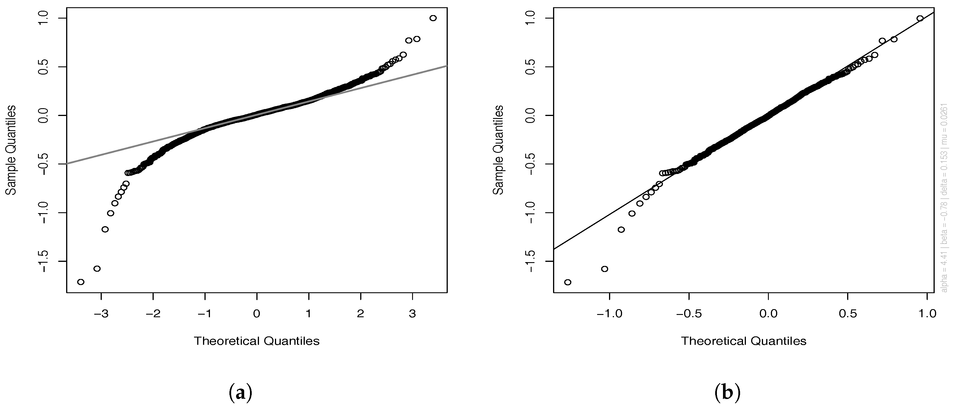
In Benth and Benth (2004), the authors performed an analysis on oil and natural gas prices, showing that the normal inverse Gaussian (NIG) process is appropriate to model the residuals of the logarithmic spot prices. Looking at the quantile-quantile (QQ) plot for our residuals in Figure 1b, we see how the theoretical NIG quantiles fit the sample ones, except for the left tail. Nevertheless, comparing this plot with the theoretical Gaussian quantiles in Figure 1a, we can notice how the NIG quantiles perform better than the Gaussian ones. Hence, we choose the process L to follow a normal inverse Gaussian distribution, although the QQ plot shows a deviation in the left tail, unexplained by the NIG. Other kinds of processes can be considered in order to better capture this behavior unexplained by our chosen process.

Let us recall some definitions. From Benth and Benth (2004), we know that an NIG process with parameters $(\alpha ,\beta ,\mu ,\delta )$ is characterized by a Lévy measure $\nu$ of the form:

$$\nu (dx)=f(x;\alpha ,\beta ,\delta )dx,$$

(4)

where:

$$f(x;\alpha ,\beta ,\delta ):=\frac{\delta \alpha }{\pi \left|x\right|}exp\left(\beta x\right)J_1\left(\alpha \left|x\right|\right).$$

(5)

Here, $x\in \mathbb{R},\mu \in \mathbb{R},\delta >0,0\le \left|\beta \right|\le \alpha$, and $J_1$ is the modified Bessel function of the third kind and Index 1; see (Jørgensen 1982, Appendix) for more details. Moreover, the parameters $(\alpha ,\beta ,\mu ,\delta )$ can be explained as follows: $\alpha$ is the steepness parameter, and a larger $\alpha$ gives a steeper density; $\beta$ is an asymmetry parameter, and $\beta =0$ gives a symmetric density; $\delta$ is a scale; and $\mu$ is a location parameter.

Calibration

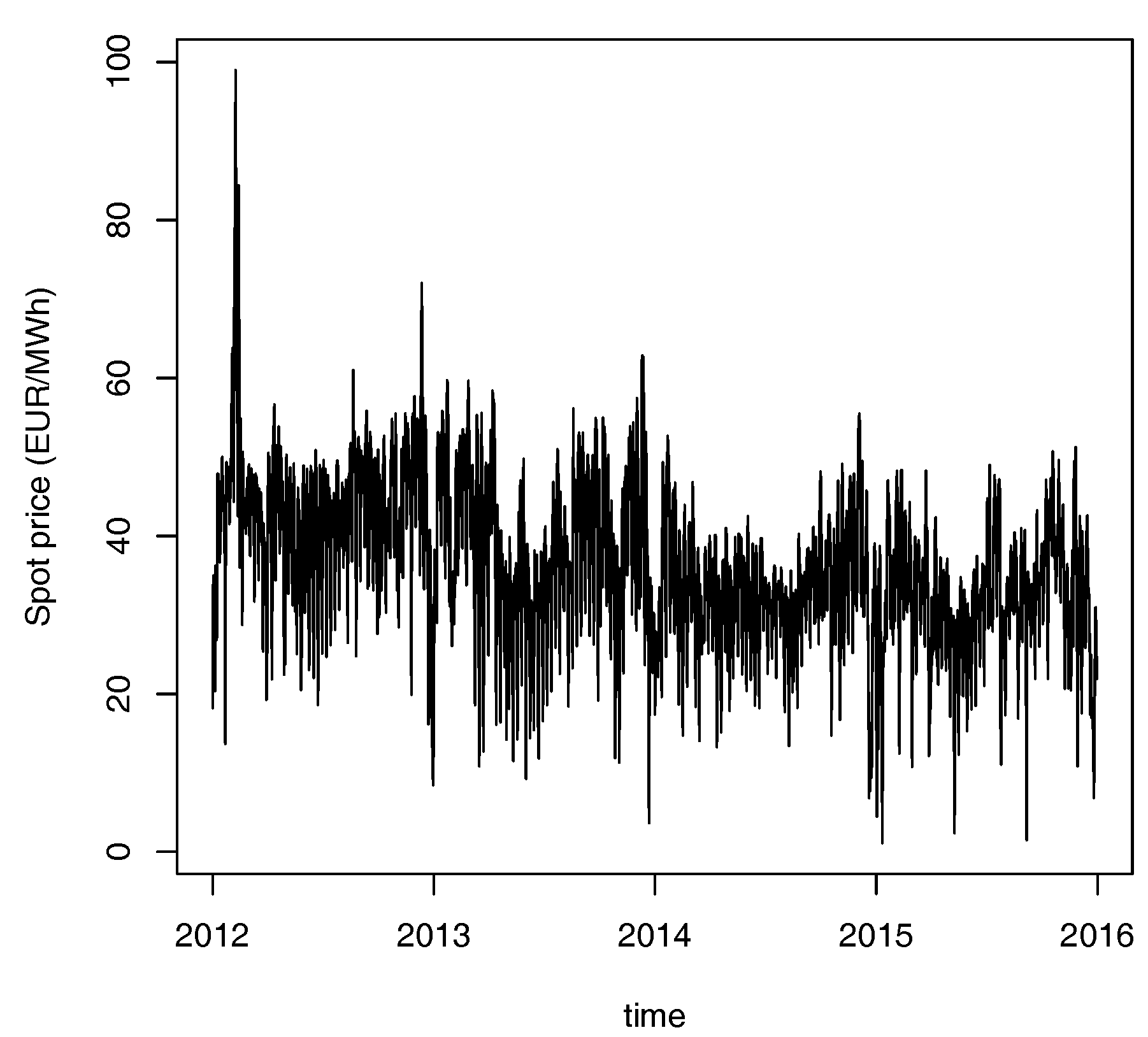
For the spot price, we consider the Phelix Day Base (PDB) index time series from the European Power Exchange (EPEX) Spot Daily indices (EUR/MWh). In particular, we consider daily data for the period from 1 January 2012–31 December 2015, for a total of 1460 daily observations, removing 29 February 2012. The eight negative values (0.55% of the total observations) in the series have been predicted by interpolation. Aiming at studying the time series $S_k:=S(t_k)$, for:

$$t_k=k,k=1,\dots ,1460,$$

(6)

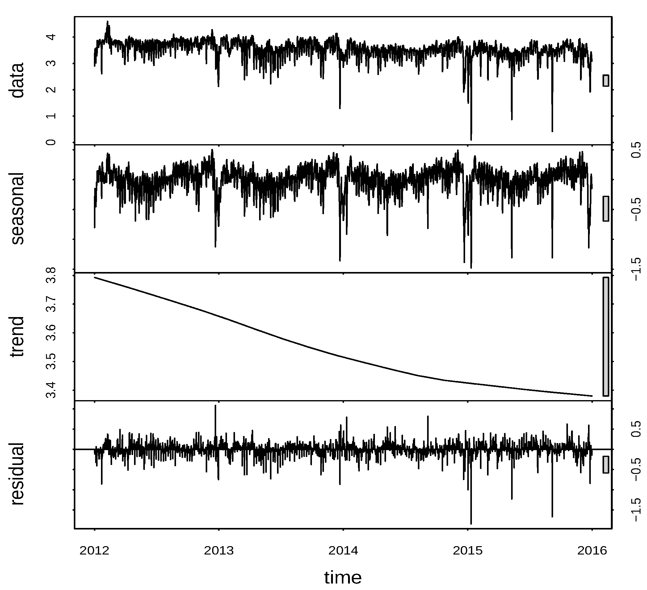
we start by considering its logarithm, namely $log(S_k)$, which, by Equation (1), can be represented by the sum $log(S_k)=log({\Lambda }_S(t_k))+K(t_k)$. We then extract1 from $log(S_k)$ the three components: trend, seasonal and remainder, which can be seen in Figure 2. However, in this paper, we will not study the trend and seasonal components, as we are interested in analyzing only the stochastic part. Hence, considering $log({\Lambda }_S(t_k))$ to be the sum of the trend and seasonal components, which are deterministic, we focus on the stochastic component, $K_k:=K(t_k)$, by means of Equation (3).

For $t_0=0$ and $t=t_k$, $k\ge 1$, it becomes:

$$K_k=e^{-{\theta }_{S}k}{K}_0+e^{-{\theta }_{S}k}{\int }_0^k{e}^{{\theta }_{S}s}dL(s),$$

(7)

where $K_0:=K(0)$, and we set ${ϵ}_{k,K}:=e^{-{\theta }_{S}k}{\int }_{k-1}^k{e}^{{\theta }_{S}s}dL(s)$, so that, by the additivity property of the stochastic integral, we can rewrite $K_k$ in Equation (7) as:

$$K_k=\varphi K_{k-1}+{ϵ}_{k,K}, \mathrm{where} \varphi :=e^{-{\theta }_S}.$$

(8)

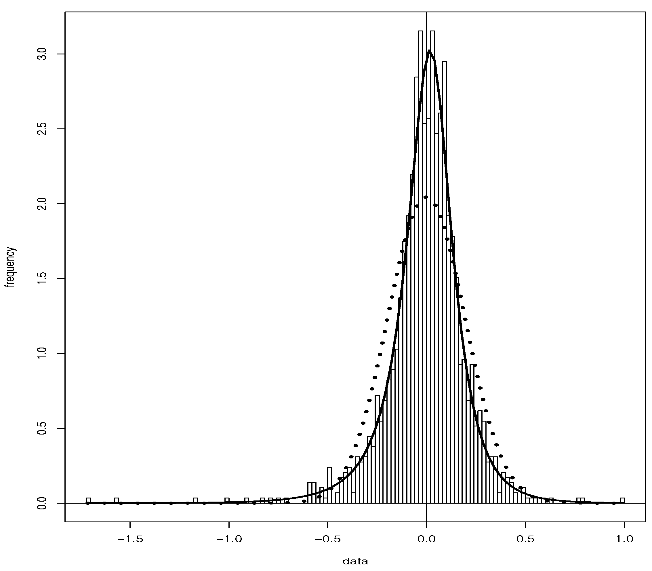
Hence, the discrete process $K_k$ is seen to be an auto-regressive model of order one (AR$(1)$) with parameter $\varphi$ and random noise ${ϵ}_{k,K}$. Denoting by $\widehat{\varphi }$ the estimate of $\varphi$2, from Equation (8), we get ${\widehat{\theta }}_S=-log\widehat{\varphi }$, whose estimated value is reported in

Table 1. Estimated parameters for the electricity spot price process.

	Estimate	Confidence interval (95%)		Estimate	Confidence interval (95%)
${\widehat{\theta }}_S$	$1.23$	$[1.08,1.42]$	${\widehat{\sigma }}_{\epsilon }$	$9.87\times {10}^{-4}$	$[9.13,10.5]\times {10}^{-4}$
$\widehat{\alpha }$	$4.41$	$[3.49,5.33]$	$\widehat{\mu }$	$2.61\times {10}^{-2}$	$[1.24,3.99]\times {10}^{-2}$
$\widehat{\beta }$	$-7.80\times {10}^{-1}$	$[-12.8,-2.77]\times {10}^{-1}$	$\widehat{\delta }$	$1.53\times {10}^{-1}$	$[1.33,1.73]\times {10}^{-1}$

, while we indicate with ${\widehat{ϵ}}_{k,K}$ the estimated residuals time series, which due to our assumptions, is driven by the NIG Lévy process L. By the maximum likelihood estimation (MLE) method, we estimate3 the NIG parameters $(\alpha ,\beta ,\mu ,\delta )$ by $(\widehat{\alpha },\widehat{\beta },\widehat{\mu },\widehat{\delta })$, whose values are reported in Table 1 along with the $95\%$ confidence intervals4, while Figure 3 shows how the bell-shaped curve of the estimated NIG distribution (bold line) fits the sample data better than the estimated Gaussian distribution (dotted line).

3. Models for Wind

Betz’s law states that the power production from a wind power plant is proportional to the cubic wind speed; see Betz (1966). According to Burton (2011), we can also assume that there is no power generation during too high/low wind regimes, as the power plant needs a minimum wind speed, called the cut-in wind speed, in order to start, and it must be stopped if the wind speed reaches a certain maximum threshold, called the cut-out wind speed, above which the wind turbines risk breakage. If we introduce $m\in {\mathbb{R}}^{+}$ as the minimum wind speed for having production and $M\in {\mathbb{R}}^{+}$ as the maximum one, we can express the wind power production P in terms of the wind speed W by the following function:

$$P(t)=h{W}^3(t){\mathbb{I}}_{m\le W(t)\le M}.$$

(9)

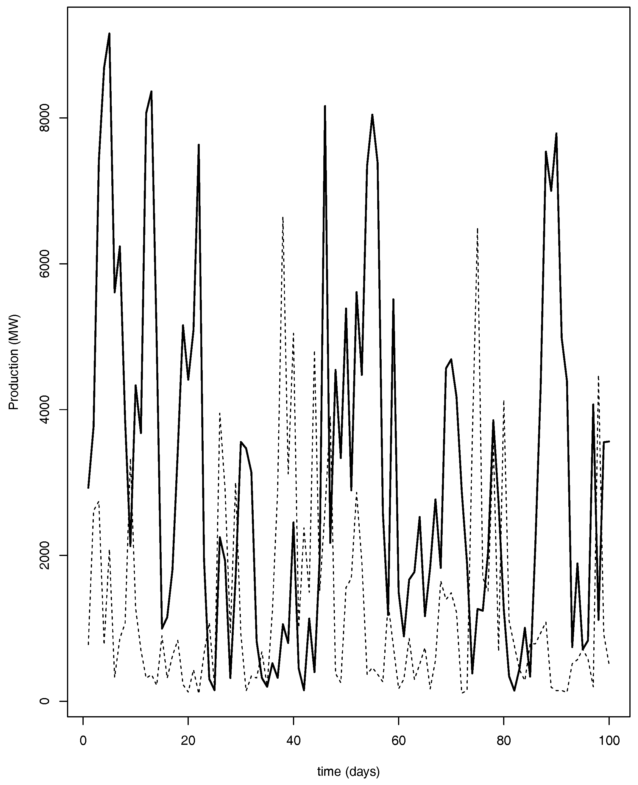
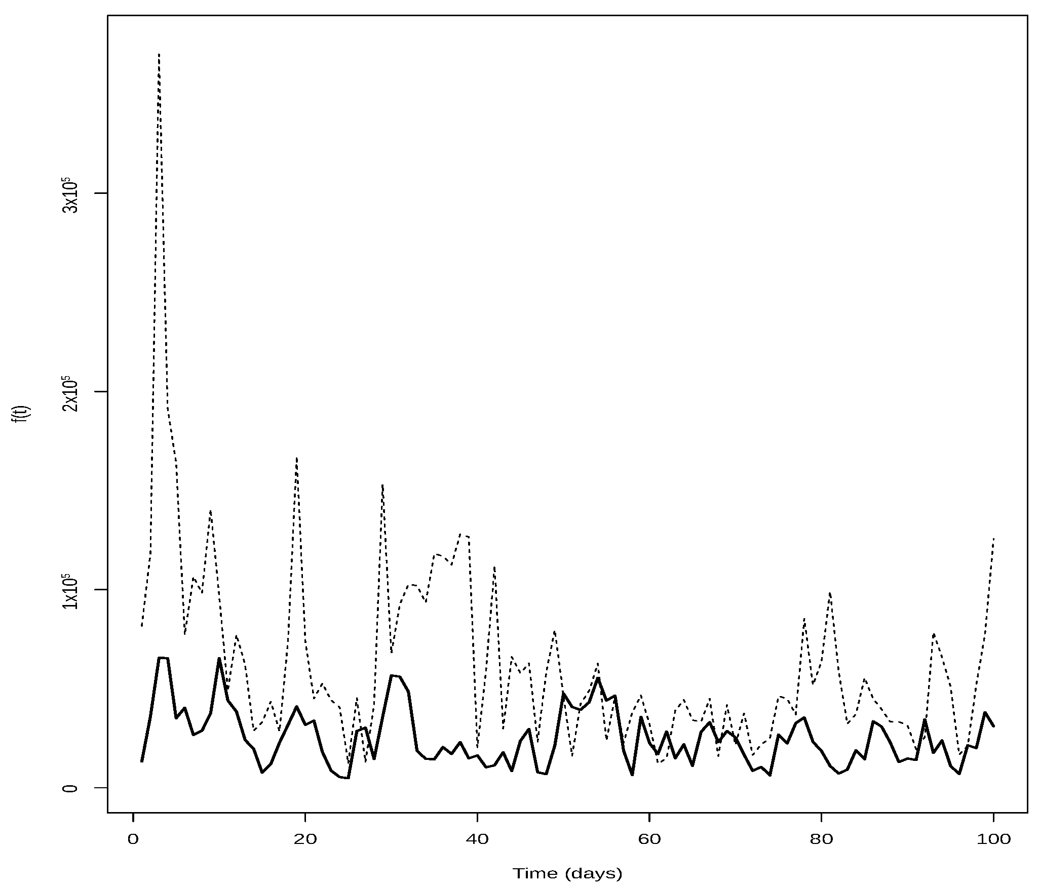
Here, h is the heat rate, being a real positive constant measuring the efficiency of the plant, which depends, e.g., on the area of the rotor blades, on the energy loss in the turbine, on humidity, etc.; see Burton (2011) for details. It also depends on the number of wind turbines in the plant. However, missing this information, considering the time series for the power production and for the cubic wind speed, we can calibrate h using a linear regression model5 for the Betz law in Equation (9), where we define the cut-in wind speed, respectively the cut-out wind speed to be such that $m=0$ and $M=+\infty$, and the indicator function ${\mathbb{I}}_{m\le W(t)\le M}$ is constantly equal to one. In particular, for the wind speed, we consider the data series from the Karlsruhe Institute of Technology, measured at 100 m above the ground (m/s), together with the data retrieved from www.50hertz.com for the wind power production (MW). Considering the same time interval as in Section 2, to work at the same resolution level, for the wind power production, the daily observations are obtained taking the average over the available 96 values per each day, i.e., referred to quarters of an hour. Then, we transform the time series from MW to MWh. The value obtained for $\widehat{h}$ starting from these time series is in

Table 2. Betz’s law parameters.

$m=0$

$M=+\infty$

$\widehat{h}=8.42\pm 0.38\times {10}^6$

. In Figure 4, we report the power production time series (dotted line) obtained from the wind speed time series by the Betz law, using the parameters in Table 2, against the real power production (bold line), with respect to the first one hundred days in order to better capture the difference between the two curves. In particular, Figure 4 shows some differences between the two curves. We think that these differences can be addressed to the historical time series used for the calibration, as the power production time series does not refer to the same geographical area of the wind speed time series. Indeed, the measuring mast of the Karlsruhe Institute of Technology (KIT) is located at the coordinates 49°5′33″ N, 8°25′33″ E, that is in the southwest part of Germany, while the grid of 50 Hertz refers to the northeast part of the country, as can be seen in the map available in the web site, www.50hertz.com. Moreover, the value for the heat rate h has been estimated, as the real one was not available. In order to have it, we would need to know the total number of wind turbines and their dimensions. Let us also remark that the Betz law gives a theoretical maximum portion of power that can be extract from an airstream flowing through the turbine at a given speed in a certain time instant t. However, here, we are considering daily observations; hence, our time is discrete and not continuous, and the wind speed may vary during a period of time. In order to take into account this effect, we refer to Villanueva and Andrés (2010), where the wind speed probability density function is considered in order to write an equation for the mean power transported by the airstream and the mean maximum power that can be extracted with a rotor. Moreover, as explained in Burton (2011), for each plant, we can also define the so-called capacity factor, which is given by the ratio between the energy delivered over a certain period and the energy that would have been supplied if the plant had operated at its maximum rate. Considering all these factors, we can obtain a more precise model; however, this is beyond the scope of this study.

By means of relation (9), we can perform two different approaches for P in our study, either to model the wind speed W or to model the power production P directly. Following Benth et al. (2008), we consider in both cases an Ornstein–Uhlenbeck (OU) process for the stochastic component of these two wind variables. In what follows, we will develop explicitly the modeling and the calibration for W: the same steps and results hold for P.

We consider the stochastic process W to be modeled by the following equation:

$$W(t)={\Lambda }_W(t)e^{X_W(t)},t\ge t_0\ge 0,$$

(10)

where ${\Lambda }_W$ is a deterministic function whose logarithm represents the seasonal component of the logarithm of W, while $X_W$ is the OU process driven by:

$$d{X}_W(t)=-{\theta }_W{X}_W(t)dt+{\sigma }_{W}dB(t),$$

(11)

for ${\theta }_W,{\sigma }_W>0$ constant parameters and B Brownian motion. By the Itô–Doeblin formula, we can prove that the process:

$$X_W(t)=e^{-{\theta }_W(t-t_0)}{X}_W(t_0)+{\sigma }_W{\int }_{t_0}^t{e}^{-{\theta }_W(t-s)}dB(s)$$

(12)

is the solution of the SDE in (11). It follows that the process $X_W$ has a Gaussian distribution with conditional mean and variance respectively given by:

$$\begin{array}{c}{\mu }_{X,W}(t):=\mathbb{E}\left[\left.X_W(t)\right|{\mathcal{F}}_{t_0}\right]=e^{-{\theta }_W(t-t_0)}{X}_W(t_0),\hfill \end{array}$$

(13)

$$\begin{array}{c}{\sigma }_{X,W}^2(t):=\mathrm{Var}(\left.X_W(t)\right|{\mathcal{F}}_{t_0})=\frac{{\sigma }_W^2}{2{\theta }_W}\left(1-e^{-2{\theta }_W(t-t_0)}\right).\hfill \end{array}$$

(14)

Analogous results hold for P. In particular, the Brownian motion B in the wind power production dynamics is considered to be the same one as for the wind speed dynamics, Equation (11). This is due to the fact that the amount of energy produced is proportional to the cubic wind speed, as stated by the Betz law, Equation (9); hence, P and W can be considered as driven by the same factor.

Calibration

Introducing $W_k:=W(t_k)$, for $t_k$ as in Equation (6), we start by considering the logarithm of the wind speed time series, which by means of Equation (10), can be written as $log(W_k)=log\left({\Lambda }_W(t_k)\right)+X_W(t_k)$. We set $log\left({\Lambda }_W(t_k)\right)$ to be the sum of the seasonal and trend components6 and $X_k:=X_W(t_k)$ to be the series of the remainders. We want to calibrate this latter series by means of Equation (11). From now on, we omit the index W, referring to the fact that the same holds for $X_P$, the stochastic component of P. In particular, we indicate with X the process that can be either $X_W$ or $X_P$, then $\theta \in \{{\theta }_W,{\theta }_P\}$ and $\sigma \in \{{\sigma }_W,{\sigma }_P\}$. Considering $t_0=0$ and $t=t_k$, Equation (12) becomes:

$$X_k=e^{-\theta k}{X}_0+\sigma e^{-\theta k}{\int }_0^k{e}^{\theta s}dB(s),$$

where $X_0:=X(0)$, and setting ${ϵ}_{k,X}:=\sigma e^{-\theta k}{\int }_{k-1}^k{e}^{\theta s}dB(s)$, we write the discrete process $X_k$ as an AR$(1)$ given by:

$$X_k=\psi X_{k-1}+{ϵ}_{k,X},\mathrm{where}\psi :=e^{-\theta }.$$

(15)

Moreover, ${ϵ}_{k,X},k\ge 1$, are i.i.d. Gaussian random variables with mean zero and variance:

$${\sigma }_{ϵ,X}^2:=\frac{{\sigma }^2}{2\theta }\left(1-e^{-2\theta }\right).$$

(16)

Indicating with $\widehat{\psi }$, respectively by ${\widehat{\sigma }}_{ϵ,X}^2$, the estimates of $\psi$ and ${\sigma }_{ϵ,X}^2$7, by Equation (15), we get $\widehat{\theta }=-log\widehat{\psi }$, while Equation (16) gives us ${\widehat{\sigma }}^2=\frac{2\widehat{\theta }{\widehat{\sigma }}_{ϵ,X}^2}{1-e^{-2\widehat{\theta }}}$, whose values, according to our datasets, are reported in

Table 3. Estimated parameters from the calibration of the wind speed and wind power production time series.

	Estimate	Confidence Interval (95%)		Estimate	Confidence Interval (95%)
${\widehat{\theta }}_W$	$7.97\times {10}^{-1}$	$[7.00,9.04]\times {10}^{-1}$	${\widehat{\theta }}_P$	$5.90\times {10}^{-1}$	$[5.16,6.71]\times {10}^{-1}$
${\widehat{\sigma }}_W^2$	$1.15\times {10}^{-1}$	$[1.07,1.24]\times {10}^{-1}$	${\widehat{\sigma }}_P^2$	$4.93\times {10}^{-1}$	$[4.59,5.31]\times {10}^{-1}$

, for both W and P.

4. Income for a Wind Energy Company

The stylized income at time $t_0\ge 0$ from a wind power plant up to time $t\in [t_0,T]$, for $T\in \left(t_0,+\infty \right)$, is given by the expected value of the discounted product of the power production P and the spot price S, namely:

$$V_0:=\mathbb{E}\left[\left.{\int }_{t_0}^t{e}^{-r(s-t_0)}P(s)S(s)ds\right|{\mathcal{F}}_{t_0}\right]={\int }_{t_0}^t{e}^{-r(s-t_0)}{f}_P(s)ds,$$

(17)

where $f_P(t):=\mathbb{E}\left[\left.P(t)S(t)\right|{\mathcal{F}}_{t_0}\right]$ and for an $r>0$ constant risk-free interest rate. In particular, we price this income under the real-world probability $\mathbb{P}$. By Equation (9), $V_0$ can also be expressed in terms of the wind speed W:

$$V_0=\mathbb{E}\left[\left.{\int }_{t_0}^t{e}^{-r(s-t_0)}h{W}^3(s){\mathbb{I}}_{m\le W(s)\le M}S(s)ds\right|{\mathcal{F}}_{t_0}\right]={\int }_{t_0}^t{e}^{-r(s-t_0)}{f}_W(s)ds,$$

(18)

where $f_W(t):=\mathbb{E}\left[\left.h{W}^3(t){\mathbb{I}}_{\{m\le W(t)\le M\}}S(t)\right|{\mathcal{F}}_{t_0}\right]$. Then, by Equations (1) and (10), we can rewrite $f_P$ and $f_W$ by:

$$\begin{array}{c}{f}_P(t)={\Lambda }_P(t){\Lambda }_S(t)\mathbb{E}\left[\left.e^{X_P(t)+K(t)}\right|{\mathcal{F}}_{t_0}\right],\hfill \end{array}$$

(19)

$$\begin{array}{c}{f}_W(t)=h{\Lambda }_W^3(t){\Lambda }_S(t)\mathbb{E}\left[\left.e^{3X_W(t)+K(t)}{\mathbb{I}}_{\{a(t)\le X_W(t)\le A(t)\}}\right|{\mathcal{F}}_{t_0}\right],\hfill \end{array}$$

(20)

where $a(t):=log\left(\frac{m}{{\Lambda }_W(t)}\right)$ and $A(t):=log\left(\frac{M}{{\Lambda }_W(t)}\right)$, for $t\ge t_0$. Let us recall that NIG processes are of pure-jump type, as the continuous martingale part in their Lévy–Khintchine representation is zero; see, e.g., Benth et al. (2008); or Tankov and Cont (2004). Therefore, an NIG process cannot be correlated with a Brownian motion, as this is a continuous process. On the other hand, spot price and wind power production are two correlated processes. In order to reproduce this correlation, we split the Lévy process into two additive components as suggested in Asmussen and Rosiński (2011), one Brownian-driven representing the small jumps of L and the other one Lévy driven for the bigger jumps, but independent of the first one and of the wind Brownian component. We introduce this approximation in the next subsection.

4.1. Normal Inverse Gaussian Approximation

In Asmussen and Rosiński (2011), the authors introduced for $\epsilon >0$ an approximation $L_{\epsilon }$ for the NIG Lévy process L with Lévy measure $\nu$ in Equation (4) as the sum of a scaled Brownian motion $B_L$ and a compound Poisson process $C_L$, namely:

$$L_{\epsilon }(t):={\sigma }_{\epsilon }{B}_L(t)+C_L(t),t\ge 0,$$

(21)

where ${\sigma }_{\epsilon }$ is the variation of the small jumps of L given by:

$${\sigma }_{\epsilon }^2:={\int }_{\left|x\right|<\epsilon }{x}^2\nu (dx),$$

(22)

while $C_L$ is independent of $B_L$ and with Lévy measure ${\nu }_{\epsilon }(dx)$ defined by:

$${\nu }_{\epsilon }(dx):=\nu (dx){\mathbb{I}}_{\left|x\right|\ge \epsilon }.$$

(23)

To measure the accuracy for the approximation (21) and to have a criterion for the selection of $\epsilon$, Asmussen and Rosiński (2011, Theorem 3.1) suggest that the difference between the distribution function for $L(1)$ and for $L_{\epsilon }(1)$ can be estimated by the quantity:

$$\underset{x\in \mathbb{R}}{sup}|\mathbb{P}(L_{\epsilon }(1)\le x)-\mathbb{P}(L(1)\le x)|\le 0.7975{\delta }_{\epsilon },$$

(24)

with ${\delta }_{\epsilon }:={\sigma }_{\epsilon }^{-3}{\int }_{\left|x\right|<\epsilon }{\left|x\right|}^3\nu (dx)$. Then, starting from the estimated parameters for the NIG Lèvy process L in Table 1, by Equations (4) and (5), we approximate ${\sigma }_{\epsilon }^2$ in Equation (22) by:

$${\widehat{\sigma }}_{\epsilon }^2=\frac{\widehat{\delta }\widehat{\alpha }}{\pi }{\int }_{\left|x\right|<\epsilon }\left|x\right|exp\left(\widehat{\beta }x\right)J_1\left(\widehat{\alpha }\left|x\right|\right)dx,$$

where $J_1$ is defined for $x>0$; hence, we split the domain of integration into two parts excluding zero, respectively $(-\epsilon ,0^{-})$ and $(0^{+},\epsilon )$. In Table 1, we report ${\widehat{\sigma }}_{\epsilon }$ obtained for $0^{\pm }=\pm {10}^{-10}$ and $\epsilon ={10}^{-5}$, where this latter choice has been taken in relation to Equation (24) in order to get an approximation error of order ${10}^{-3}$. Similarly, by Equation (23), the estimated Lévy measure for $C_L$ is given by:

$${\widehat{\nu }}_{\epsilon }(dx)=\frac{\widehat{\delta }\widehat{\alpha }}{\pi \left|x\right|}exp\left(\widehat{\beta }x\right)J_1\left(\widehat{\alpha }\left|x\right|\right){\mathbb{I}}_{\left|x\right|\ge \epsilon }dx.$$

(25)

With the approximation in Equation (21), we can easily make $L_{\epsilon }$ dependent on the wind noise through the Brownian motion $B_L$.

4.2. Income Formulas

Introducing the processes:

$$\begin{array}{c}Y(t):=e^{-{\theta }_S(t-t_0)}Y(t_0)+{\sigma }_{\epsilon }{\int }_{t_0}^t{e}^{{\theta }_S(t-s)}d{B}_L(s),\hfill \end{array}$$

(26)

$$\begin{array}{c}Z(t):={\int }_{t_0}^t{e}^{{\theta }_S(t-s)}d{C}_L(s),\hfill \end{array}$$

(27)

with $Y(t_0):=K(t_0)$, the Ornstein–Uhlenbeck process K in Equation (3) can be written by the sum:

$$K(t)=Y(t)+Z(t),t\ge t_0\ge 0,$$

(28)

where, in particular, Y and Z are independent because of the independence of $B_L$ and $C_L$. Let us also mention that the process Y as defined in Equation (26) has a Gaussian distribution with conditional mean and variance respectively given by:

$$\begin{array}{c}{\mu }_Y(t):=\mathbb{E}\left[\left.Y(t)\right|{\mathcal{F}}_{t_0}\right]=Y(t_0)e^{-{\theta }_S(t-t_0)},\hfill \end{array}$$

(29)

$$\begin{array}{c}{\sigma }_Y^2(t):=\mathrm{Var}(\left.Y(t)\right|{\mathcal{F}}_{t_0})=\frac{{\sigma }_{\epsilon }^2}{2{\theta }_S}\left(1-e^{-2{\theta }_S(t-t_0)}\right).\hfill \end{array}$$

(30)

Considering $B_L$ to be correlated with the Brownian motion B in the OU wind dynamics, Equation (11), with constant correlation $\rho \in [-1,1]$, we find the correlation function c between Y and W$(P)$ to be given by:

$$c(t):=\mathrm{Corr}(X(t),Y(t))=2\rho \frac{\sqrt{\sigma {\sigma }_{\epsilon }}}{\theta +{\theta }_S}·\frac{1-e^{-(\theta +{\theta }_S)(t-t_0)}}{\sqrt{1-e^{-2\theta (t-t_0)}}\sqrt{1-e^{-2{\theta }_S(t-t_0)}}}.$$

(31)

In particular, by Equation (28) and the independence of Z with both X and Y, we can rewrite $f_P$ and $f_W$ in Equation (19), respectively Equation (20), as follows:

$$\begin{array}{c}{f}_P(t)={\Lambda }_P(t){\Lambda }_S(t)\mathbb{E}\left[\left.e^{X_P(t)+Y(t)}\right|{\mathcal{F}}_{t_0}\right]\mathbb{E}\left[\left.e^{Z(t)}\right|{\mathcal{F}}_{t_0}\right],\hfill \end{array}$$

(32)

$$\begin{array}{c}{f}_W(t)=h{\Lambda }_W^3(t){\Lambda }_S(t)\mathbb{E}\left[\left.e^{3X_W(t)+Y(t)}{\mathbb{I}}_{\{a(t)\le X_W(t)\le A(t)\}}\right|{\mathcal{F}}_{t_0}\right]\mathbb{E}\left[\left.e^{Z(t)}\right|{\mathcal{F}}_{t_0}\right].\hfill \end{array}$$

(33)

Let us introduce the functions:

$$\begin{array}{c}{f}_{XY}^P(t):={\Lambda }_P(t){\Lambda }_S(t)\mathbb{E}\left[\left.e^{X_P(t)+Y(t)}\right|{\mathcal{F}}_{t_0}\right],\hfill \end{array}$$

(34)

$$\begin{array}{c}{f}_{XY}^W(t):=h{\Lambda }_W^3(t){\Lambda }_S(t)\mathbb{E}\left[\left.e^{3X_W(t)+Y(t)}{\mathbb{I}}_{\{a(t)\le X_W(t)\le A(t)\}}\right|{\mathcal{F}}_{t_0}\right],\hfill \end{array}$$

(35)

$$\begin{array}{c}{f}_Z(t):=\mathbb{E}\left[\left.e^{Z(t)}\right|{\mathcal{F}}_{t_0}\right],\hfill \end{array}$$

(36)

for which the following results hold:

Proposition 1.

The analytical expression for$f_{XY}^P$in Equation (34) is given by:

$$f_{XY}^P(t)={\Lambda }_P(t){\Lambda }_S(t)exp\left\{\frac{1}{2}{\Sigma }_P^2(t)+\left({\mu }_{X,P}(t)+{\mu }_Y(t)\right)\right\},$$

(37)

where ${\Sigma }_P^2(t):=\left(1+2c(t)\right){\sigma }_{X,P}^2(t)+{\sigma }_Y^2(t)$.

Proof. 

The proof is straightforward. ☐

Proposition 2.

The analytical expression for$f_{XY}^W$in Equation (35) is given by:

$$f_{XY}^W(t)=h{\Lambda }_W^3(t){\Lambda }_S(t)\left[\Phi (d(t,M))-\Phi (d(t,m))\right]exp\left\{\frac{1}{2}{\Sigma }_W^2(t)+\left(3{\mu }_{X,W}(t)+{\mu }_Y(t)\right)\right\},$$

(38)

with ${\Sigma }_W^2(t):=3\left(3+2c(t)\right){\sigma }_{X,W}^2(t)+{\sigma }_Y^2(t)$, and Φ the cumulative standard Gaussian distribution function, while for $w\in \{m,M\}$, we define:

$$d(t,w):=\frac{log\left(\frac{w}{{\Lambda }_W(t)}\right)-{\mu }_{X,W}(t)}{{\sigma }_{X,W}(t)}-(3+c(t)){\sigma }_{X,W}(t),$$

(39)

for $c(t)$ in Equation (31).

Proof. 

The proof is straightforward. ☐

Proposition 3.

The analytical expression for$f_Z$in Equation (36) is given by:

$$f_Z(t)=exp\left\{{\int }_{t_0}^t\Psi (s)ds\right\},$$

(40)

with:

$$\Psi (s):={\int }_{-\infty }^{\infty }\left(e^{e^{-{\theta }_S(t-s)}x}-1\right){\nu }_{\epsilon }(dx),$$

(41)

where ${\nu }_{\epsilon }(dx)$ is the Lévy measure for the compound Poisson process $C_L$, Equation (23).

Proof. 

See Appendix A. ☐

By means of Equations (38) and (37), we can evaluate $f_{XY}^W$ and $f_{XY}^P$ using the values in Table 1, Table 2 and Table 3. We need to take into account that, starting from the wind speed time series in m/s, by the Betz law, we obtain a time series for the production that is determined in watts (W). We thus need to convert it into megawatt hours (MWh), as the spot price time series is in EUR/MWh. Then, let us focus on $f_Z$. By Equations (4), (25), (40) and (41), we get ${\widehat{f}}_Z(t)=exp\left(g(t)\right)$ for:

$$g(t):={\int }_{t_0}^t{\int }_{\left|x\right|\ge \epsilon }\left(e^{e^{-{\widehat{\theta }}_S(t-s)}x}-1\right)\frac{\widehat{\delta }\widehat{\alpha }}{\pi \left|x\right|}exp\left(\widehat{\beta }x\right)J_1\left(\widehat{\alpha }\left|x\right|\right)dxds,$$

and for $t_0=0$ and $t=t_k$, we have ${\widehat{f}}_Z(t_k)=exp\left(g(t_k)\right)$, where:

$$g(t_k)={\int }_0^{k-1}{\int }_{{(-\epsilon ,\epsilon )}^C}\left(e^{e^{-{\widehat{\theta }}_S(k-s-1)}x}-1\right)\frac{\widehat{\delta }\widehat{\alpha }}{\pi \left|x\right|}exp\left(\widehat{\beta }x\right)J_1\left(\widehat{\alpha }\left|x\right|\right)dxds,$$

(42)

for which the following holds:

Proposition 4.

The approximated value for$g(t_k)$in Equation (42) can be obtained by $g_k$ defined by the recursion:

$$\left\{\begin{array}{c}{g}_1=0\hfill \\ g_k=g_{k-1}+\frac{1}{2}\left\{h_{k-1}+h_{k-2}\right\},k\ge 2\hfill \end{array}\right.,$$

being $h_k$ defined by:

$$h_k:={\int }_{{(-\epsilon ,\epsilon )}^C}\left(e^{e^{-{\widehat{\theta }}_{S}k}x}-1\right)\frac{\widehat{\delta }\widehat{\alpha }}{\pi \left|x\right|}exp\left(\widehat{\beta }x\right)J_1\left(\widehat{\alpha }\left|x\right|\right)dx,k\ge 0.$$

Proof. 

Let us consider Equation (42): for $k=1$, we get $g_1=0$, while for $k\ge 2$, we can use the trapezoidal rule with step $\Delta =1$, together with the linearity of stochastic integrals, in order to get the recursion. ☐

Hence, by the estimate of $h_k$8, we can also estimate $g_k$ and consequently ${\widehat{f}}_Z(t_k)$ by ${\widehat{f}}_Z^k=exp(g_k)$. Then, from Equations (32) and (33), we get $f_P$ and $f_W$. In Figure 5, we report the estimated $f_P$ (bold line) and $f_W$ (dotted line) with respect to one hundred days to better capture the difference between the two curves. We can notice that $f_P$ is mostly lower than $f_W$. This means that, according to our datasets, the forecasted income from a wind power plant will be higher if calculated with respect to the wind speed. Remember indeed that the income is given by Equations (17) and (18), respectively. Let us notice that the difference obtained between these two functions can also be due to the different geographical areas to which the time series for the wind speed and the power production are related; see Section 3 for more details.

5. Quanto Options

In Section 3, we introduced the Betz law, which gives a theoretical maximum value for the power that can be extracted from the wind airstream that passes through the wind turbine. Nevertheless, this maximum is never achieved in reality, and practically, a power plant yields only a certain percentage of such a power. Let us think for example that, due to reciprocal positions of the turbines in a plant, there will be much turbulence in the wake of one turbine, creating a different wind structure for the next, and so on, and in particular, we can think that this phenomenon depends on the design of the plant itself. We can also think that the time itself affects the efficiency of a wind turbine. As damages at the plant imply less energy production, less energy production means less income. Moreover, as the power production is proportional to the cubic wind speed, less wind gives less production. In what follows, we are going to construct a European put-type quanto option to cover against such risks, as well as the price risks. We mainly follow Benth et al. (2013).

Before proceeding, let us say a few words about the pricing measure. So far, we have modeled and priced under the real-world probability measure $\mathbb{P}$. However, when it comes to pricing a derivative contract, a risk-neutral probability measure $\mathbb{Q}$ is introduced in order to take into account the risk-premium and to ensure the absence of arbitrage opportunities. Namely, we need to consider a pricing measure $\mathbb{Q}$ to gain the martingale property for the underlying tradable discounted price processes. Nevertheless, in the context of energy markets, electricity is not a storable asset; hence, it cannot be traded in the usual way as it must be consumed once produced. This means that the underlying spot cannot be liquidly bought and kept in a portfolio. For this reason, electricity cannot be considered a traded asset, and the electricity spot price is not taken into account when fixing the pricing measure. Hence, in this context, any probability measure $\mathbb{Q}$ equivalent to the real-world probability $\mathbb{P}$ can be considered as a pricing measure. On the other hand, futures markets are liquid, and futures contracts must have an arbitrage-free price dynamics; see (Benth et al. 2008, sct. 1.5) for more details. A particular choice of pricing measure is simply $\mathbb{Q}=\mathbb{P}$. We use this choice here as any other will require the modeling of the risk premium. Using $\mathbb{Q}=\mathbb{P}$ gives a benchmark price that can be used to study the risk premium.

5.1. Contract Structure

The double-hedging property of quanto options implies that the payoff function depends on the two underlying assets. Let us indicate with $\pi (E,I)$ the payoff function being dependent on the energy price index E and on an index of power production I. In particular, considering the period $[{\tau }_1,{\tau }_2]$, with ${\tau }_1<{\tau }_2$, we define E to be the average spot price, namely:

$$E:=\frac{1}{{\tau }_2-{\tau }_1}\sum _{t={\tau }_1}^{{\tau }_2}S(t),$$

(43)

while I is the cumulative gap between the theoretical total maximum production given by the Betz law in Equation (9) according to the measured wind speed W and the registered power production P, namely:

$$I:=\sum _{t={\tau }_1}^{{\tau }_2}\left(h{W}^3(t)-P(t)\right),$$

(44)

where we included the assumptions $m=0,M=+\infty$ (see Table 2), in order to simplify the resulting formulas. Indeed for $d(t,w)$ in Equation (39), we get $d(t,0)=-\infty$ and $d(t,+\infty )=+\infty$, which lead to $\Phi (d(t,+\infty ))-\Phi (d(t,0))=1$ in Equation (38). Let us notice that the terms in the sum of Equation (44) are all at least non-negative, being the Betz law an upper bound for the power production, so that we do not need to take the absolute value of the terms in the sum.

As defined in Benth et al. (2013), if the option is exercised at time ${\tau }_2$, its arbitrage-free price at time $t_0\le {\tau }_2$ is given by the discounted expected value of the payoff function, namely:

$${\Pi }_0:=e^{-r({\tau }_2-t_0)}\mathbb{E}\left[\left.\pi (E,I)\right|{\mathcal{F}}_{t_0}\right],$$

(45)

$r>0$ being the risk-free interest rate. Following Benth et al. (2013), we relate this price to futures contracts based on the same indices. In particular, the prices at time $t_0\le {\tau }_2$ of futures contracts written on the index E, respectively I with delivery period $[{\tau }_1,{\tau }_2]$, are given by:

$$\begin{array}{c}{F}_{t_0}^E({\tau }_1,{\tau }_2)=\mathbb{E}\left[\left.\frac{1}{{\tau }_2-{\tau }_1}\sum _{t={\tau }_1}^{{\tau }_2}S(t)\right|{\mathcal{F}}_{t_0}\right],\hfill \end{array}$$

(46)

$$\begin{array}{c}{F}_{t_0}^I({\tau }_1,{\tau }_2)=\mathbb{E}\left[\left.\sum _{t={\tau }_1}^{{\tau }_2}\left(h{W}^3(t)-P(t)\right)\right|{\mathcal{F}}_{t_0}\right].\hfill \end{array}$$

(47)

Let us notice that the future $F_{t_0}^I({\tau }_1,{\tau }_2)$ can also be seen like the difference between two different futures contracts: the first one written on the cubic wind speed and the second one on the power production, namely:

$$F_{t_0}^I({\tau }_1,{\tau }_2)=\mathbb{E}\left[\left.\sum _{t={\tau }_1}^{{\tau }_2}h{W}^3(t)\right|{\mathcal{F}}_{t_0}\right]-\mathbb{E}\left[\left.\sum _{t={\tau }_1}^{{\tau }_2}P(t)\right|{\mathcal{F}}_{t_0}\right]=F_{t_0}^W({\tau }_1,{\tau }_2)-F_{t_0}^P({\tau }_1,{\tau }_2).$$

The following Lemma can be proven:

Lemma 1.

The price of a quanto option whose payoff is a function of the two indices E and I is the same as another option whose payoff is a function of the terminal values of two futures contracts written on the same indices and with a delivery period equal to the period specified by the option, namely Equation (45) is equivalent to:

$${\Pi }_0=e^{-r({\tau }_2-t_0)}\mathbb{E}\left[\left.\pi \left(F_{{\tau }_2}^E({\tau }_1,{\tau }_2),F_{{\tau }_2}^I({\tau }_1,{\tau }_2)\right)\right|{\mathcal{F}}_{t_0}\right].$$

(48)

Proof. 

For $t_0={\tau }_2$, we get $F_{{\tau }_2}^E({\tau }_1,{\tau }_2)=E$ and $F_{{\tau }_2}^I({\tau }_1,{\tau }_2)=I$, i.e. the futures price at the terminal time is equal to what is being delivered. ☐

Therefore, we consider the quanto option as written on two futures contracts traded as financial assets. Moreover, we define the payoff function $\pi$ as the product between two put derivatives:

$$\pi \left(F_{{\tau }_2}^E({\tau }_1,{\tau }_2),F_{{\tau }_2}^I({\tau }_1,{\tau }_2)\right):=max\left(H_E-F_{{\tau }_2}^E({\tau }_1,{\tau }_2),0\right)\times max\left(H_I-F_{{\tau }_2}^I({\tau }_1,{\tau }_2),0\right),$$

(49)

where $H_E,H_I>0$ are the respective strike values. Such a payoff function allows the buyer to cover against low prices, but also against low wind power production from the plant. The put-put contract is then interesting from the point of view of a wind power producer; nevertheless, the put-call or the call-call cases can be similarly considered. In order to calculate the expectation in Equation (48), we need to model the futures price dynamics $F_{t_0}^E({\tau }_1,{\tau }_2)$ and $F_{t_0}^I({\tau }_1,{\tau }_2)$.

5.2. Futures Dynamics

Let us focus on the futures contracts introduced in Equations (46) and (47). Considering the models introduced in Section 2 and Section 3 for the spot price and the wind dynamics, the following results hold:

Lemma 2.

For$t_0<{\tau }_1$, the futures value (46) takes the form:

$$F_{t_0}^E({\tau }_1,{\tau }_2)=\frac{1}{{\tau }_2-{\tau }_1}\sum _{t={\tau }_1}^{{\tau }_2}{\Lambda }_S(t)exp\left\{{\mu }_Y(t)+\frac{1}{2}{\sigma }_Y^2(t)+{\int }_{t_0}^t\Psi (s)ds\right\},$$

(50)

while for $t_0=T$, ${\tau }_1\le T\le {\tau }_2$, we get:

$$F_T^E({\tau }_1,{\tau }_2)=\frac{1}{{\tau }_2-{\tau }_1}\sum _{t={\tau }_1}^{T}S(t)+\frac{1}{{\tau }_2-{\tau }_1}\sum _{t=T+1}^{{\tau }_2}{\Lambda }_S(t)exp\left\{{\mu }_Y(t)+\frac{1}{2}{\sigma }_Y^2(t)+{\int }_{t_0}^t\Psi (s)ds\right\},$$

(51)

being ${\mu }_Y$ and ${\sigma }_Y$ the mean, respectively the variance, of the process Y given in Equation (29), respectively Equation (30), and Ψ the function defined in Equation (41).

Proof. 

By Equations (1) and (28) and Theorem 3, we can write that:

$$\mathbb{E}\left[\left.S(t)\right|{\mathcal{F}}_{t_0}\right]={\Lambda }_S(t)\mathbb{E}\left[\left.e^{Y(t)+Z(t)}\right|{\mathcal{F}}_{t_0}\right]={\Lambda }_S(t)exp\left\{{\mu }_Y(t)+\frac{1}{2}{\sigma }_Y^2(t)+{\int }_{t_0}^t\Psi (s)ds\right\},$$

being Y normally distributed with mean ${\mu }_Y$ and variance ${\sigma }_Y$ and independent from Z, so that the first result is proven. Moreover, for ${\tau }_1\le T\le {\tau }_2$, we can split the sum in Equation (46) into what is known, that is for $t\le T$, and what is not known, that is for $t>T$:

$$F_T^E({\tau }_1,{\tau }_2)=\mathbb{E}\left[\left.\frac{1}{{\tau }_2-{\tau }_1}\sum _{t={\tau }_1}^{T}S(t)\right|{\mathcal{F}}_T\right]+\mathbb{E}\left[\left.\frac{1}{{\tau }_2-{\tau }_1}\sum _{t=T+1}^{{\tau }_2}S(t)\right|{\mathcal{F}}_T\right].$$

Then, since ${\sum }_{t={\tau }_1}^{T}S(t)$ is ${\mathcal{F}}_T$-measurable, for the first term, we can drop the conditional expectation, while for the second one, we refer to the previous step. ☐

Lemma 3.

For$t_0<{\tau }_1$, the futures values (47) are obtained by:

$$F_{t_0}^I({\tau }_1,{\tau }_2)=h\sum _{t={\tau }_1}^{{\tau }_2}{\Lambda }_W^3(t)exp\left(3{\mu }_{X,W}(t)+\frac{9}{2}{\sigma }_{X,W}^2(t)\right)-\sum _{t={\tau }_1}^{{\tau }_2}{\Lambda }_P(t)exp\left({\mu }_{X,P}(t)+\frac{1}{2}{\sigma }_{X,P}^2(t)\right),$$

(52)

while for $t_0=T$, ${\tau }_1\le T\le {\tau }_2$, we get:

$$\begin{array}{c}{F}_T^I({\tau }_1,{\tau }_2)=h\left(\sum _{t={\tau }_1}^T{W}^3(t)+\sum _{t=T+1}^{{\tau }_2}{\Lambda }_W^3(t)exp\left(3{\mu }_{X,W}(t)+\frac{9}{2}{\sigma }_{X,W}^2(t)\right)\right)+\\ -\left(\sum _{t={\tau }_1}^{T}P(t)+\sum _{t=T+1}^{{\tau }_2}{\Lambda }_P(t)exp\left({\mu }_{X,P}(t)+\frac{1}{2}{\sigma }_{X,P}^2(t)\right)\right),\end{array}$$

(53)

for ${\mu }_{X,W}$ and ${\sigma }_{X,W}^2$, ${\mu }_{X,P}$ and ${\sigma }_{X,P}^2$ given in Equation (13), respectively Equation (14).

Proof. 

We refer to Lemma 2. ☐

Let us define now the contract details, namely we fix the drafting date, $t_0$, the measurement period, $[{\tau }_1,{\tau }_2]$ (see

Table 4. Quanto option measurement period.

$t_0$:	31/12/2014
${\tau }_1$:	01/01/2015
${\tau }_2$:	31/12/2015

), and the yearly free-risk interest rate, $r=1\%$. In particular, we decided to consider $t_0<{\tau }_1$; the case ${\tau }_1<t_0<{\tau }_2$ can be similarly obtained. Let us notice that, usually, such a type of contract is characterized by more than one strike price. Indeed, the time of measurement $[{\tau }_1,{\tau }_2]$ is usually divided into sub-intervals, typically of one month length, and for each sub-interval, different values for $H_I$ and $H_E$ are defined. This structure is tailor made in order to take into account the seasonal behavior of the variables involved. Indeed, e.g., in the case of a quanto option written on the heating degree days (HDD) index, we can think that the strike price for November will be different from the one for January; see, for example, (Benth and Benth 2004, Table 1). Here, we do not split the measurement period $[{\tau }_1,{\tau }_2]$ into sub-intervals, but we consider the option to be at-the-money instead, which means the strikes $H_I$ and $H_E$ are set to be equal, respectively, to $F_{t_0}^I({\tau }_1,{\tau }_2)$ and $F_{t_0}^E({\tau }_1,{\tau }_2)$. Furthermore, for each of these calibrations, we use five different values for the correlation $\rho \in \{-0.9,-0.5,0,0.5,0.9\}$, in order to see whether this parameter affects the price of the option. Finally, we perform three different calibrations: the first one exploiting the datasets from 1 January 2012–31 December 2014, the second one from 1 January 2013–31 December 2014 and the third one from 1 January 2014–31 December 2014, being 31 December 2014 the drafting day. By this, we want to observe whether there are any differences in the price values with respect to different lengths of the historical sets used.

Exploiting the calibration procedures performed in Section 4, we can estimate $F_{t_0}^E({\tau }_1,{\tau }_2)$ in Equation (50), and for T varying in the interval $[{\tau }_1,{\tau }_2]$, we obtain the vector ${\widehat{\mathbf{F}}}_E({\tau }_1,{\tau }_2)=\left[{\widehat{F}}_{{\tau }_1}^E({\tau }_1,{\tau }_2),\dots ,{\widehat{F}}_{{\tau }_2}^E({\tau }_1,{\tau }_2)\right]$ of realizations for $F_T^E({\tau }_1,{\tau }_2)$. In particular, for the first sum in Equation (51), we use the values referring to the year 2014: indeed, since our contract is stipulated on 31 December 2014, we do not have at our disposal the 2015 time series; therefore, we exploit the data belonging to the preceding year. Similarly, we estimate $F_{t_0}^I({\tau }_1,{\tau }_2)$ in Equation (52), and we obtain the vector ${\widehat{\mathbf{F}}}_I({\tau }_1,{\tau }_2)$ of realizations of $F_T^I({\tau }_1,{\tau }_2)$, for $T\in [{\tau }_1,{\tau }_2]$.

Let us focus now on the dynamics for the two futures contracts $F_T^E({\tau }_1,{\tau }_2)$ and $F_T^I({\tau }_1,{\tau }_2)$ for $T\in [{\tau }_1,{\tau }_2]$. We can notice that in Equation (51), the second term is a sum of exponential functions, where the exponent has the form ${\mu }_Y(t)+\frac{1}{2}{\sigma }_Y^2(t)+{\int }_{t_0}^t\Psi (s)ds$, for $t\in [T+1,{\tau }_2]$. Being ${\mu }_Y(t)$ dependent on $Y(t_0)$, which is normally distributed, its exponential has a log-normal distribution. In particular, we know that the sums of log-normal distributed random variables are not log-normally distributed. The same holds for Equation (52). Nevertheless, in order to simplify the calibration and the pricing of the quanto option, we decide to model $F_T^E({\tau }_1,{\tau }_2)$ and $F_T^I({\tau }_1,{\tau }_2)$ with two log-normal distributed processes. Let us introduce for $t_0\le T\le {\tau }_2$ the following dynamics for the futures prices:

$$\begin{array}{c}{F}_T^E({\tau }_1,{\tau }_2)=F_{t_0}^E({\tau }_1,{\tau }_2)exp({\mu }_E+Z_E),\hfill \end{array}$$

(54)

$$\begin{array}{c}{F}_T^I({\tau }_1,{\tau }_2)=F_{t_0}^I({\tau }_1,{\tau }_2)exp({\mu }_I+Z_I),\hfill \end{array}$$

(55)

where $Z_E$ and $Z_I$ are two ${\mathcal{F}}_{t_0}$-independent Gaussian random variables with correlation $\rho :=\mathrm{Corr}(Z_E,Z_I)$. Moreover, we let $Z_E$ and $Z_I$ have zero mean and variance defined by ${\sigma }_E^2:=\mathrm{Var}(Z_E)$ and ${\sigma }_I^2:=\mathrm{Var}(Z_I)$. In particular, since the futures price is a martingale under the measure $\mathbb{Q}$, it can be proven that ${\mu }_E=-\frac{{\sigma }_E^2}{2}$ and ${\mu }_I=-\frac{{\sigma }_I^2}{2}$.

5.3. Option Price

By means of Equations (54) and (55), we derive the following result:

Theorem 1.

The market price at time$t_0$of a European energy quanto option written on assets following the dynamics given in Equations (54) and (55), with payoff defined as in Equation (49) and exercised at time ${\tau }_2$, given by:

$$\begin{array}{cc}{\Pi }_0& =e^{-r({\tau }_2-t_0)}\left(H_E{H}_I\Phi (x_1,y_1;\rho )-H_I{F}_{t_0}^E({\tau }_1,{\tau }_2)\Phi (x_2,y_2;\rho )+\right.\hfill \\ & \left.-H_E{F}_{t_0}^I({\tau }_1,{\tau }_2)\Phi (x_3,y_3;\rho )+F_{t_0}^E({\tau }_1,{\tau }_2)F_{t_0}^I({\tau }_1,{\tau }_2)e^{\rho {\sigma }_E{\sigma }_I}\Phi (x_4,y_4;\rho )\right),\hfill \end{array}$$

(56)

with:

$$\begin{array}{c}{x}_1:=\frac{log\left(\frac{H_I}{F_{t_0}^I({\tau }_2,{\tau }_1)}\right)+\frac{{\sigma }_I^2}{2}}{{\sigma }_I},y_1:=\frac{log\left(\frac{H_E}{F_{t_0}^E({\tau }_2,{\tau }_1)}\right)+\frac{{\sigma }_E^2}{2}}{{\sigma }_E},\hfill \\ x_2:=x_1-\rho {\sigma }_I,x_3:=x_1-{\sigma }_E,x_4:=x_1-{\sigma }_E-\rho {\sigma }_I,\hfill \\ y_2:=y_1-{\sigma }_I,y_3:=y_1-\rho {\sigma }_E,y_4:=y_1-{\sigma }_I-\rho {\sigma }_E.\hfill \end{array}$$

Here, $\Phi (x,y;\rho )$ denotes the standard bivariate Gaussian cumulative distribution function with correlation ρ.

Proof. 

The proof in (Benth et al. 2013, Proposition 3.1) for the call-call payoff function can be easily adapted to our put-put case. ☐

Starting from ${\widehat{F}}_{t_0}^E({\tau }_1,{\tau }_2)$ and ${\widehat{\mathbf{F}}}_E({\tau }_1,{\tau }_2)$, by Equation (54), we then estimate ${\sigma }_E^2$ by ${\widehat{\sigma }}_E^2=\mathrm{Var}\left(log\left(\frac{{\widehat{\mathbf{F}}}_E({\tau }_1,{\tau }_2)}{{\widehat{F}}_{t_0}^E({\tau }_1,{\tau }_2)}\right)\right)$, and we get the vector of realizations for $Z_E$ as ${\widehat{\mathbf{Z}}}_E=log\left(\frac{{\widehat{\mathbf{F}}}_E({\tau }_1,{\tau }_2)}{{\widehat{F}}_{t_0}^E({\tau }_1,{\tau }_2)}\right)+\frac{{\widehat{\sigma }}_E^2}{2}$. Similarly, starting from ${\widehat{F}}_{t_0}^I({\tau }_1,{\tau }_2)$ and ${\widehat{\mathbf{F}}}_I({\tau }_1,{\tau }_2)$, by Equation (55), we estimate ${\sigma }_I^2$, and we get the vector of realizations for $Z_I$. The value used for $\widehat{h}$ is in Table 2. Let us notice that all the steps performed in this section have been applied three times, with respect to the three different calibration periods. Moreover, considering the option at-the-money, that is $H_E=F_{t_0}^E({\tau }_1,{\tau }_2)$ and $H_I=F_{t_0}^I({\tau }_1,{\tau }_2)$, Equation (56) becomes:

$$\begin{array}{cc}{\Pi }_0& =e^{-r({\tau }_2-t_0)}{F}_{t_0}^I({\tau }_1,{\tau }_2)F_{t_0}^E({\tau }_1,{\tau }_2)·\hfill \\ & \left(\Phi (x_1,y_1;\rho )-\Phi (x_2,y_2;\rho )-\Phi (x_3,y_3;\rho )+e^{\rho {\sigma }_E{\sigma }_I}\Phi (x_4,y_4;\rho )\right).\hfill \end{array}$$

In

Table 5. Quanto option prices.

$\mathit{\rho }$	Three-Year Calibration		Two-Year Calibration		One-Year Calibration
$-0.9$	$15.25$	$(-96.73\%)$	$270.76$	$(-95.94\%)$	$419.21$	$(-95.56\%)$
$-0.5$	$163.15$	$(-65.02\%)$	$2459.24$	$(-63.11\%)$	$3559.76$	$(-62.28\%)$
0	$466.43$	$(0\%)$	$6666.03$	$(0\%)$	$9437.49$	$(0\%)$
$0.5$	$882.27$	$(89.15\%)$	$12,253.93$	$(83.83\%)$	$17,143.00$	$(81.65\%)$
$0.9$	$1309.76$	$(180.80\%)$	$17,920.39$	$(168.83\%)$	$24,911.99$	$(163.967\%)$

, we report our results. In particular, in the columns, we have the three different calibrations, which are: three-year calibration, from 1 January 2012–31 December 2014; two-year calibration, from 1 January 2013–31 December 2014; one-year calibration, from 1 January 2014–31 December 2014; while in the rows, we used different values for the correlation $\rho$. In parenthesis, we report the percentage change in the price considering the corresponding value for $\rho =0$ as an indicator. Finally, in

Table 6. Correlations estimated in the three different settings.

Three-Year Calibration	Two-Year Calibration	One-Year Calibration
$\widehat{\rho }=4.53\times {10}^{-1}$	$\widehat{\rho }=8.58\times {10}^{-1}$	$\widehat{\rho }=8.32\times {10}^{-1}$

, we report the actual correlation values obtained from the calibrations.

Looking at the numerical results listed in Table 5, we can notice that in the three-year calibration, the prices are significantly lower with respect to the other two columns. Moreover, we can see how the price is affected from the value of the correlation. Indeed, for each of the three calibrations, the prices increase as the correlation increases, being lowest when the correlation is close to $-1$ and highest when the correlation is close to $+1$. Looking at the percentage changes in parenthesis, we can also notice that the biggest changes with respect to the case $\rho =0$ are for a highly positive correlation and that these percentage changes are similar in the three different calibration settings, that is reading the table by rows. From the definition of the payoff function for the quanto option in Equation (49), we can argue that the changes in the prices in Table 5 agree with such a definition. In fact, the payoff function pays more when both $F_{{\tau }_2}^E({\tau }_1,{\tau }_2)<<H_E$ and $F_{{\tau }_2}^I({\tau }_1,{\tau }_2)<<H_I$, that is when the futures prices are far lower than the respective strike values, while it pays less if only one of these conditions is satisfied. If the correlation $\rho$ is negative, this means that when one of the futures contract value is decreasing, the other one is going in the opposite direction instead, leading to low values for the quanto option. On the contrary, when $\rho$ is positive and the futures price dynamics decreases, the other one is decreasing, as well, leading to high values for the option. The dependency of the option price from the correlation parameter confirms that it is important to model the correlation between the two futures dynamics, $F_T^E({\tau }_1,{\tau }_2)$ and $F_T^I({\tau }_1,{\tau }_2)$. In our model, such a correlation has be considered to be constant; nevertheless, a more sophisticated model can be considered instead.

In Table 6, we report the correlation values obtained from the three different calibrations performed. As we can see, the value obtained in the three-year calibration is quite different in the module from the other two. We cannot give a formal interpretation of such a result, but a possible explanation could be in the spot price time series itself. Indeed, from Figure 6, we can notice this big jumps behavior at the beginning of 2012, which may affect the correlation with the wind power production process. We think that this can be also a possible explanation for the different price values obtained in the three-year calibration (Table 5, first column); nevertheless, a deeper study should be performed in order to better understand the nature of this different correlation value. Let us notice also that the estimated $\rho$ has positive value, which means the two futures contracts are positively correlated. Looking at Equations (43) and (44), we can argue that this is in line with the definition of the two indices E and I. Indeed, when the difference $h{W}^3(t)-P(t)$ is small, it means that the power plant has captured a big portion of the energy transported by the wind stream, as the difference between the Betz law for the maximum production and the actual production is small. At the same time, more production may lead to lower electricity prices. Hence, low values for I may be related to low values for E. Similarly, high values for I may be related to high values for E. Nevertheless, a deeper study in this sense should be also performed.

6. Conclusions

We first modeled the residuals of the log-spot price by an NIG Lévy process, while the wind speed and wind power production have been modeled by two OU processes. With the intent of modeling the correlation between the electricity spot price and the wind power production, we considered an approximation of the NIG process given by a scaled Brownian motion and a compound Poisson process, following Asmussen and Rosiński (2011). This has allowed us to correlate the NIG process with the OU process, which in principle cannot be, being the first one a pure-jump process, while the second a process with continuous paths. In particular, considering the Betz law, which links wind power production and wind speed by a cubic law, two possible approaches have been possible: modeling the power production directly, or the wind speed first. We then applied our bivariate models to price the income from a wind power plant. As shown in Figure 5, we obtained higher income if considering the wind speed as the wind variable, instead of the wind power production directly. We infer that a possible reason for such a difference is related to the particular datasets used in this paper, as the geographical area to which the wind speed is related is not the same as for the production; see Section 3 for the discussion about that. We then constructed a European put-type quanto option that allows a wind energy producer to hedge against the loss of income due to the volume risk in terms of reduced production, as well as against the price risk. Following the approach used in Benth and Benth (2004), we have priced the quanto option, whose value has been linked to futures contracts on the energy and wind production indices. This is advantageous since futures are traded financial assets. Finally, we found numerical values for the price of our contract, with respect to different settings, highlighting that the correlation is influential when pricing quanto options. The correlation between the two futures contracts is indeed important, since the payoff function is depending on the two contracts in a nonlinear way.

More sophisticated models for the futures dynamics can be introduced, as we considered two log-normal distributed processes with constant mean and variance, while the mean and variance can be seen as stochastic processes themselves. Moreover, as we included a Lèvy component in the dynamics of the spot price, the same can be in principle done for the wind processes, as also these processes may present some non-Gaussianity. We would like to underline that model improvements can be achieved, e.g., considering a wind density function as suggested in Villanueva and Andrés (2010), as well as deeply analyzing the correlation factor and its stochastic description. Finally, a more rigorous analysis can be performed having more precise datasets, as well as more detailed information about the power plants involved.

References

- Applebaum, David. 2009. Lévy Processes and Stochastic Calculus. Cambridge Studies in Advanced Mathematics. Cambridge: Cambridge University Press. [Google Scholar] [CrossRef]
- Asmussen, Søren, and Jan Rosiński. 2011. Approximations of Small Jumps of LéVy Processes with a View towards Simulation. Journal of Applied Probability 38: 432–93. [Google Scholar]
- Benth, Fred E., and Jūratė Š. Benth. 2004. The Normal Inverse Gaussian distribution and spot price modeling in energy markets. International Journal of Theoretical and Applied Finance 7: 177–92. [Google Scholar] [CrossRef]
- Benth, Fred E., and Jūratė Š. Benth. 2012. Modeling and Pricing in Financial Markets for Weather Derivatives. Singapore: World Scientific. [Google Scholar]
- Benth, Fred E., Jūratė Š. Benth, and Steen Koekebakker. 2008. Stochastic Modelling of Electricity and Related Markets. Singapore: World Scientific. [Google Scholar]
- Benth, Fred E., Nina Lange, and Tor Åge Myklebust. 2013. Pricing and hedging quanto options in energy markets. Journal of Energy Markets 8: 1–35. [Google Scholar] [CrossRef]
- Betz, Albert. 1966. Introduction to the Theory of Flow Machines. Oxford: Pergamon Press. [Google Scholar]
- Burton, Tony. 2011. Wind Energy: Handbook. Hoboken: John Wiley & Sons. [Google Scholar]
- Folland, Gerald B. 2007. Real Analysis: Modern Techniques and Their Applications, 2nd ed. Hoboken: Wiley. [Google Scholar]
- Jørgensen, Bent. 1982. Statistical Properties of the Generalised Inverse Gaussian Distribution. Lecture Notes in Statistics. New York: Springer, vol. 9. [Google Scholar]
- Schwartz, Eduardo S. 1997. The stochastic behavior of commodity prices: Implication for valuation and hedging. The Journal of Finance 52: 923–73. [Google Scholar] [CrossRef]
- Tankov, Peter, and Rama Cont. 2004. Financial Modeling with Jump Processes. CRC Financial Mathematics Series; Boca Raton: CRC Press. [Google Scholar]
- Villanueva, Daniel, and Feijoó Andrés. 2010. Wind power distributions: A review of their applications. Renewable and Sustainable Energy Reviews 14: 1490–95. [Google Scholar] [CrossRef]
- Wystup, Uwe. 2010. Quanto Options. In Encyclopedia of Quantitative Finance. Hoboken: Wiley. [Google Scholar] [CrossRef]