A Least-Squares Monte Carlo Framework in Proxy Modeling of Life Insurance Companies


1
Department of Mathematics, TU Kaiserslautern, Erwin Schrödinger Strasse, Geb. 48, 67653 Kaiserslautern, Germany
2
Mathematical Institute, University Cologne, Weyertal 86-90, 50931 Cologne, Germany
3
Department Financial Mathematics, Fraunhofer ITWM, Fraunhofer-Platz 1, 67663 Kaiserslautern, Germany
*
Author to whom correspondence should be addressed.
Risks 2018, 6(2), 62; https://doi.org/10.3390/risks6020062
Submission received: 29 March 2018
/
Revised: 5 June 2018
/
Accepted: 7 June 2018
/
Published: 11 June 2018
(This article belongs to the Special Issue Capital Requirement Evaluation under Solvency II framework)
Abstract
:The Solvency II directive asks insurance companies to derive their solvency capital requirement from the full loss distribution over the coming year. While this is in general computationally infeasible in the life insurance business, an application of the Least-Squares Monte Carlo (LSMC) method offers a possibility to overcome this computational challenge. We outline in detail the challenges a life insurer faces, the theoretical basis of the LSMC method and the necessary steps on the way to a reliable proxy modeling in the life insurance business. Further, we illustrate the advantages of the LSMC approach via presenting (slightly disguised) real-world applications.
1. Introduction
The standards set out in the Solvency II directive mark the starting point for the recent developments of proxy modeling to calculate solvency capital requirements in the insurance sector, see European Parliament and European Council (2009). As noted in Article 122 of the latter document:
“Where practicable, insurance and reinsurance undertakings shall derive the solvency capital requirement directly from the probability distribution forecast generated by the internal model of those undertakings, using the Value-at-Risk measure set out in Article 101(3).”
The crucial point of this quotation is that the insurers are asked to derive their full loss distributions. A common understanding is that, for a reasonably accurate full distribution, several hundred thousand simulations are necessary. Moreover, for each of these simulations, for with profit business at least 1000 Monte Carlo valuations must be carried out. This leaves the insurance companies with the requirement to perform hundreds of millions of own funds calculations to obtain their full loss distributions.
The mere fact that such an extensive calculation is foreseen in the directive shows that, in the years preceding the Solvency II directive, it was believed that by the time Solvency II would be introduced much lower hardware costs and increased valuation efficiency would allow European life insurance companies to perform that many simulations. Since the industry as of today is still far away from such computational capacities, the companies face the challenge to find suitable approximation techniques. Among them are sophisticated techniques such as Least-Squares Monte Carlo (LSMC), which we focus on in this paper. The central idea of LSMC is to get along with comparably few Monte Carlo simulations and to estimate the desired values by least-squares regression.
Let us return to the probability distribution forecast mentioned in the directive. Which are major considerations affecting a company’s own funds and thus its loss distribution? Life insurance constitutes a long-term business. Take a typical annuity policy: It is a life-long contract which may be written when a person is 25 years old. It will be in the books of the insurer potentially for 60 years or more. To assess the potential losses from a portfolio of such policies, it does not suffice to look at the profits or losses in the current year or in the last five or ten years. The policyholder may pay her premiums without receiving any benefits for decades and decades. From a company’s perspective, it will only become clear whether it has made profits or losses from this policy after the policy has expired, either cancelled or due to the policyholder’s death. This assessment gets even more complicated by the regulatory frameworks. In more complex business regulations, such as in Germany, the company has to assure it will have enough assets to cover the expected annuity payments during the entire lifetime of the policy. Furthermore, each year it has to set aside a sufficient provision for the future benefits taking into account the interest rate guarantees promised to the customer.
For this purpose, each policy is projected into the future. The provisions are built and released as stipulated, and the annuity payments performed until expiration, all according to the actuarial tables. The software used for projecting the policies is variously called actuarial platform, stochastic model or cash flow projection model. We stick to the last of these notions throughout this article. It is obviously an enormous challenge to make assumptions about the world in 50 or 60 years from now. The most relevant actuarial assumptions such as mortality rates, expenses or lapse behavior of customers are derived according to industry-wide standard approaches. They are largely based on historical data and contain certain assumptions regarding the expected trends. The relevant market data such as interest rates or equity developments are modeled by acknowledged methods of financial mathematics.
The computational challenge we mentioned above after citing Article 122 of the Solvency II directive (European Parliament and European Council 2009) refers primarily to the cash flow projection models. The computational burden for the calculation of the solvency capital requirement is namely directly related to the complexity of the cash flow projections models. Our intention in this paper is to shed some light on how this challenge can be overcome by utilizing the LSMC approach. We divide the calculation process into four steps. In the first step, we allocate the computational capacities to the simulations that will be used to generate the own funds fitting and validation data, and run the Monte Carlo simulations of the insurer’s cash flow projection model accordingly. Conditional on the fitting data, the proxy function for the own funds is then calibrated in the second step. This step is mathematically most demanding as it offers a great variety of regression methods which must be chosen from. A good method not only reliably generates proxy functions which capture the behavior of the cash flow projection model well, but is also transparent, flexible with regard to the characteristics of the model and fast. In the third step, the proxy function is validated conditional on the validation data. Once the validation has been successful, the proxy function is passed on for evaluation to the last step, where it yields an approximation to the insurer’s full loss distribution. Finally, the solvency capital requirement is computed as a value-at-risk of that loss distribution.
The main purpose of this paper is to give a current snapshot of why and how the companies in the life insurance sector can use an LSMC-based approach to derive their full loss probability distribution forecasts. In doing so, we close the gap between theory and practice by designing a concrete algorithm along with a suitable theoretical framework. We highlight the practical considerations an insurer should make in the various necessary steps. Even though we do not have the intention of giving a step-by-step worked example, we offer numerical illustrations in which we place our focus on the proxy function calibration, validation and evaluation and compare LSMC to the directly calculated full loss distribution (nested stochastics). Finally, we address current research topics in the area of LSMC modeling for life insurance companies.
2. Cash Flow Projection Models and LSMC
The Monte Carlo valuations we deal with are performed in the cash flow projection (CFP) models. Future cash flows dependent on market development and actuarial assumptions such as benefits paid to the policyholders are calculated in these models. Those future cash flows then get discounted to obtain the company’s value or the fair value of the company’s liabilities which are used for the derivation of the loss distribution.
2.1. Cash Flow Projection Models
In the projection of life insurance policies, the cash flow projection models play a crucial role. They replicate the modeling of products, insurance contracts and assets from the administration systems. In the following sections, we take two different perspectives when discussing the CFP models.
2.1.1. Full Balance Sheet Projections
For a projection of the future cash inflows and outflows, both assets and liabilities of a company have to be modeled. In a company’s balance sheet the assets and liabilities are interlinked in a complex manner, most prominently through the profit sharing mechanism. The CFP models hence have to be able to project all of the most important balance sheet items. Particularly complicated challenges arise from businesses such as German life insurance business where the entire portfolio belongs to a single fund and the profit sharing arises not only from the investments but also from risk and expenses profit sources. This implies that the profits in a given year which are the basis for the profit sharing can be determined only after all policies have been projected.
A CFP model thus projects a company’s balance sheet. In cases where book and market values of assets differ, it calculates them both. A pair consisting of a simulation and a projection year is a knot in the CFP model. For each knot the algorithms in the model value the company’s assets and liabilities. To derive the gross profit, the CFP model projects assets and liabilities between two consecutive projection years. A CFP model can hence be understood as a full enterprise model which projects the company in its entirety.
In this view, the CFP model consists of four modules, that is building blocks:
- Assets
- Liabilities
- Capital Market
- Management Actions
At this moment for most life insurance companies their CFP models are separate tools detached from other productive systems which are used for the statutory accounts. For instance, companies typically employ assets valuation tools other than CFP models to value their assets in the business closure. Similarly, liabilities are modeled in complex administration systems which are usually too heavy for numerous Monte Carlo projections needed for Solvency II. With increased computational capacities in the future it is conceivable that both Solvency II and statutory account valuations may be done by the same model.
2.1.2. Pricing Machine
A different perspective on the CFP model arises when it is seen as a pricing machine. In this view, the company is understood as an exotic derivative which produces future cash flows, both into (premiums) and out of the company (benefits for policyholders, costs and dividends). In this sense, it resembles a financial instrument with some swap-like and option-like features:
- inflows of premiums (mostly pre-determined);
- outflow of costs (mostly pre-determined); and
- outflow of benefits and dividends (volatile, dependent on the capital market development).
The annual premium of a policyholder is in most cases constant since policyholders demand certainty about their payments to the insurance company. This lies in the nature of the insurance business: Policyholders exchange known premium payments against uncertain benefits. For endowment and annuity products, the interest rate guarantees and profit sharing mechanisms make the cash flow patterns complex. Take for instance clique style profit sharing mechanisms (policyholder profit share in a given year underlies the original guarantee). The dependency on the capital market scenarios which are used in the projections is multi faceted and the cash flows can become arbitrarily complex. It is therefore understandable why an analytic formula for the present value of the cash flows mentioned above which would enable insurance companies to easily calculate the full distribution of losses cannot be derived.
2.2. LSMC—From American Option Pricing to Capital Requirements
In this section, we present the fundamental idea behind the LSMC approach and then consider some of its particular applications in the finance and insurance business.
The Basic Idea behind LSMC
Originally introduced as a Monte Carlo alternative for pricing American or Bermudan options, the LSMC approach combines Monte Carlo methods with regression techniques (see e.g., Carriere (1996); Tsitsiklis and Van Roy (2001) and Longstaff and Schwartz (2001)). Its basic ingredients are a set of simulated evolutions of the paths of underlying stock price(s) on a discrete time grid. While for standard European options it is straight forward to calculate the resulting payoffs, averaging over them and considering the discounted average as an approximation for the option price, such an approach is not feasible for American options due to the possibility of an early exercise.
Instead, we have to follow each path of the stock price closely and have to decide at each future time instantly if it is better to exercise the option now or to continue holding it. While the intrinsic value of the option is given by its actual payoff when immediately exercised, the continuation value depends on the future performance of the stock prices. Of course, the latter is not known at the current time. This, however, is exactly where the regression techniques come into the game. As the continuation value can be expressed as discounted (conditional) expectation of the future value of the American option (given it will not be exercised immediately), it can be expressed as a typically unknown function of the current stock price. This function is then estimated via linear regression, i.e., with the help of the least-squares method (see e.g., Korn et al. (2010) for a detailed description of the full algorithm). Having obtained the regression function at future time steps, one can compare the intrinsic value of the option and the (approximation of the) continuation value by plugging the current stock price in the regression function. In this way, one can calculate the optimal exercise boundary of an American option backward from maturity to its initial time.
This LSMC technique for American options has the typical Monte Carlo advantage of beating tree methods or PDE based methods for multiple underlyings, but tends to be slow in univariate applications.
2.3. Calculating Capital Requirements
The LSMC technique, however, is not only limited to the valuation of American-style options. Bauer and Ha (2015) have extended the scope of the LSMC approach to the risk management activities of financial institutions and in particular of life insurance companies. There, the main contribution of the LSMC technique is the possibility to overcome so-called nested valuation problems.
2.3.1. Nested Valuation Problem
As outlined in Section 1, to calculate an insurance company’s capital requirement, its assets and liabilities in the CFP model have to be projected one year into the future under a large number of real-world scenarios. The obtained positions after one year have to be (re-)valued, conditional expectations (under a pricing measure!) have to be calculated. To obtain a reliable estimate for those values, for each real-world scenario numerous stochastic simulations of the company’s CFP model need to be carried out in a naive Monte Carlo approach. This approach with simulations in the simulations is called a nested valuation problem. Such a conventional approach will for most life insurance companies exceed the computational capacities. Typically life insurance companies would need hundreds of millions of simulations for an acceptably accurate nested valuation, whereas due to time and hardware constraints they typically have the capacities to perform at most a few hundred thousand simulations.
2.3.2. Least-Squares Monte Carlo Solution
Taking up the LSMC idea from American option pricing above, Bauer and Ha (2015) have suggested a way to overcome the nested valuation problem of calculating the capital requirement by the naive approach. Instead of determining option prices by Monte Carlo simulation, they simulate paths of CFP models. Similar to estimating conditional continuation values, they estimate a company’s available capital as the difference between its assets and liabilities conditional on the real-world scenarios by ordinary least-squares regression.
Thereby, they also highlight the flexibility of the LSMC approach to switch between pricing and projection, i.e., to simulate under different probability measures over disjoint time intervals. Particularly, they cope with the nested valuation problem by introducing a hybrid probability measure: While the physical measure captures the one-year real-world scenarios under which the assets and liabilities shall be evaluated, the risk-neutral measure concerns the valuations in the CFP model after the one-year time period. Key to overcoming the nested valuation problem is that the LSMC technique gets along with only few stochastic simulations per real-world scenario. Where numerous simulations can be foregone in the LSMC approach compared to the conventional approach, the approximation of the available capital by ordinary least-squares comes in.
For a better understanding, suppose the number of stochastic simulations required to reliably estimate the available capital for one real-world scenario in the conventional approach is . Then, the LSMC approach takes advantage of the idea that the required simulations do not necessarily have to be performed based on the single real-world scenario under which the available capital shall be derived. This means that the simulations can be carried out based on different real-world scenarios. The effects of the different real-world scenarios just have to be excludable by ordinary least-squares regression. By implication, we can select and perform simulations in the LSMC approach for many relevant real-world scenarios together and thereby decrease the required computational capacities tremendously compared to the conventional approach.
Compare this to the American option pricing problem where we only simulate under the risk-neutral measure. However, each scenario at time t is only followed by one price path. Starting from maturity, the continuation values in the preceding period are simply calculated via a regression over the cross-sectional payments from not exercising the option. Thus, nested simulation at each time t for each single scenario is replaced by comparing the intrinsic option value with the current stock price inserted in the just obtained regression function. In the calculation of capital requirements, we do not even have to think about the exercise problem.
3. Least-Squares Monte Carlo Model for Life Insurance Companies
In this work, we adopt the LSMC technique as described in Bauer and Ha (2015) and develop it further to meet the specific needs of proxy modeling in life insurance companies. Amongst others, Barrie and Hibbert (2011), Milliman (2013) and Bettels et al. (2014) have already given practical illustrations of the LSMC model in risk management.
We close the gap between theory and practice by developing a practical algorithm along with a suitable theoretical framework. Variants of this algorithm have already been applied successfully in many European countries and different life insurance companies under the Solvency II directive. Although this approach appears superior to other methods in the industry and the algorithm meets the demands for reliable derivations of the solvency capital requirement, various active research streams search for refinements of the proxy functions, see the last Section 6 for details.
In this section we look in detail at the necessary steps and ingredients on the way to a reliable proxy modeling using the LSMC framework. The particular steps are:
- a detailed description of the simulation setting and the required task;
- a concept for a calibration procedure for the proxy function;
- a validation procedure for the obtained proxy function; and
- the actual application of the LSMC model to forecast the full loss distribution.
We would like to emphasize that only a carefully calibrated and rigorously validated proxy function can be used in the LSMC approach. Otherwise, there is the danger of e.g., using an insufficiently good approximation or an overfitted model.
3.1. Simulation Setting
We adopt the simulation framework of Bauer and Ha (2015) and modify it where necessary to describe the current state of the implementation in the life insurance industry.
3.1.1. Filtered Probability Space
Let be a complete filtered probability space. We also assume the existence of a risk-neutral probability measure equivalent to the physical probability measure . By , we capture the real-world scenario risk an insurer faces with regard to its assets and liabilities.
We model the risk an insurer is exposed to in the next projection year by a vector , , where each component represents the stress intensity of a financial or actuarial risk factor. We refer to X under as an outer scenario. Conditional on X, we model the insurer’s uncertainty under by a time-dependent market consistent Markov process that reflects the developments of stochastic capital market variables over the projection horizon. We refer to Monte Carlo simulations for the risk-neutral valuation as inner scenarios. Each outer scenario is assigned a set of inner scenarios. Under , we can price any security by taking the expectation of its deflated cash flows. The deflation takes place with respect to the process with , where denotes the instantaneous risk-free interest rate.
The filtration of the -algebra contains the inner scenario sets, that is the sets with the financial and actuarial information over the projection horizon, and the -algebra captures solely the sets with the accumulated information up to time t.
3.1.2. Solvency Capital Requirement
An insurer is interested in its risk profile to assess its risks associated with possible business strategies. With the knowledge of how its risks influence its profit, an insurer can steer the business using an appropriate balance between risks and profits. In risk management, a special focus is given to an insurer’s loss distribution over a one-year horizon due to the Solvency II directive, compare European Parliament and European Council (2009).
We define an insurer’s available capital at time t as its market value of assets minus liabilities and abbreviate it by . Furthermore, we define its one-year profit as the difference between its deflated available capital after one year and its initial available capital, i.e.,
where constitutes an after risk result and the unique before risk result. The solvency capital requirement (SCR) is given as the value-at-risk of the insurer’s one-year losses, that is the negative of , at the confidence level . Formally, this is the -quantile of the loss distribution, i.e.,
where denotes the cumulative distribution function of the loss under . Hence, if the initial available capital is equal to SCR, the insurer is statistically expected to default only in business years. For instance, as set out in Article 101(3) of the Solvency II directive means the company will default only with probability .
3.1.3. Available Capital
Assume the projection of asset and liability cash flows occurs annually at the discrete times . Let denote the net profit (dividends and losses for the shareholders after profit sharing) at time t and let T mark the projection end. At projection start, we can express the after risk available capital conditional on the outer scenario X as
In our modeling, we approximate the under Solvency II sought-for deflated available capital after a one-year horizon by the after risk available capital (3), i.e., . In other words, we assume that an outer scenario realizes immediately after projection start and not after one year. This consideration is important as an insurance company only knows its current CFP model but not its future ones such as after one year. Each summand in the expectation on the right-hand side is a result of the characteristics of the underlying CFP model. Under the Markov assumption, such a summand takes on a value conditional on the present inner scenario component in a simulation. Mathematically speaking, the summands can be interpreted as functionals on the vector space of profit cash flows to . Each CFP model can be represented by an element of a suitable function space. As long as the risk-free interest rate enters , we can write , , so that, by linearity of expectation, Equation (3) becomes
For the sake of completeness, if we are interested in an economic variable other than the available capital such as the market value of assets or liabilities, we can proceed in principle as described above. Essentially, we would have to adjust the cash flows of the available capital in Equations (3) and (4) such that they represent the respective variable. Instead of the SCR, another economic variable such as the changes in assets or liabilities would be defined in Equation (2).
3.1.4. Fitting Points
Unlike Bauer and Ha (2015), we specially construct a fitting space on which we define the outer scenarios that are fed into the CFP model solely for simulation purposes. We call these outer scenarios fitting scenarios. The fitting scenarios should be selected such that they cover the space of real-world scenarios sufficiently well. This is important as the proxy function of the available capital or another economic variable is derived based on these scenarios. To formalize the distribution of the fitting scenarios, we introduce another physical probability measure besides . Apart from the physical measure, we adopt the filtered probability space from above so that we refer for the fitting scenarios to the space . We specify the fitting space as a d-dimensional cube
where the intervals , , indicate the domains of the risk factors. The endpoints of these intervals correspond respectively to a very low and a very high quantile of the risk factor distribution.
The set of fitting scenarios , and the number of inner scenarios a per fitting scenario need to be defined conditional on the run time of the CFP model in the given hardware architecture. Thereby, the minimum number of scenarios required to obtain reliable results needs to be guaranteed. Moreover, the calculation budget should be split reasonably between the fitting and validation computations. To allocate the fitting scenarios on , we need to specify the physical probability measure and suggest an appropriate allocation procedure.
Once the fitting scenarios have been defined, the inner scenarios per fitting scenario , must be generated. An economic scenario generator (ESG) can be employed to derive the inner scenarios. Essentially, such a generator simulates market consistent capital market variables over the projection horizon under and ensures thus risk neutrality.
When all required inner scenarios are available, the Monte Carlo simulations of the CFP model are performed. These simulations provide the results for the available capital, i.e.,
The averages of these results over the inner scenarios yield the fitting values per fitting scenario, i.e.,
In the following, we call the points , consisting of the fitting scenarios and fitting values fitting points.
3.1.5. Practical Implementation
We now outline how the theoretical framework presented above can actually be implemented in the industry.
The first step of a life insurance company is to identify the risks its business is exposed to. Some of these risks are not quantifiable and are hence excluded from the modeling in the CFP models. However, if a risk is significant for the company and can also be implemented in the CFP model, it will usually be considered. Some quantifiable risks may not be relevant for a company: A company underwriting solely risk insurance policies is not exposed to the longevity risk for instance.
In Table 1, we list the typical risks which can be implemented in the CFP model. In this example, is the number of risk factors being quantifiable and relevant for the company. While the first nine risk factors are shocks on the capital market, the remaining eight constitute actuarial risks. We model the risk factors as either additive or multiplicative stresses. For each stress, the base value is usually zero. Except for the mortality catastrophe stress, all actuarial stresses in the table can be modeled as symmetric multiplicative or additive stresses.
Some of the risk factors can depend on vectors of underlying random factors. For example, the historic interest rate movements cannot be explained reasonably well with a one-factor model, so companies use two-factor or three-factor models for implementing . They can also include risk-free rates in different currencies which increase the number of dimensions even further. Equally, the equity shock can be the outcome of several shocks of indices, if the company is exposed to different types of equity. The spread widening risk can also be multidimensional.
As far as the number of outer scenarios is concerned, it depends on the dimensionality of the fitting space and the calculation capacities. Numbers ranging from to 100,000 fitting scenarios have been seen and tested in the industry. For the inner scenarios, the natural choice would be as this would allow greater diversification among the fitting scenarios (and is in line with the original LSMC approach!). However, in the implementations we have observed , based on the observation that the benefits from the method of antithetic variates overcompensate the reduction of the fitting scenarios, for this method see ((Glasserman 2004), Section 4.2).
For the practical implementations, it is important that the fitting space in Equation (5) is a cube. This allows using low discrepancy sequences which is a powerful tool ensuring optimal usage of the scenario budget in Monte Carlo simulations. By far the most widely used are Sobol low discrepancy sequences which are easy to implement. They have a big advantage in that they ensure that each new addition of fitting points will be optimally placed in a certain sense. For details and the exact definition of what it means that a sequence has low discrepancy see Niederreiter (1992). Since a Sobol sequence is defined on the cube , we perform a linear transformation of the dimensions to map it to our fitting space .
It is worth noting that some risk factors require an ESG for the inner scenarios conditional on the fitting scenarios to be generated. In the ESG, the financial models which determine the dynamics of for instance interest rates, equity, property and credit risk are implemented. The first four risk factors from Table 1 are always modeled directly in the ESG, the next three can also be modeled in such a way. The remaining risk factors are modeled directly as input for the CFP model.
As the final step, Monte Carlo simulations of the CFP model conditional on the inner scenarios are performed leading to the non-averaged values in Equation (6) for the available capital. After averaging, we get the fitting values in Equation (7) per fitting scenario and thus the fitting points which enter the regression.
3.2. Proxy Function Calibration
We now describe how the proxy functions used for the CFP model are practically obtained.
3.2.1. Two Approximations
As stated before, Bauer and Ha (2015) have transferred the LSMC approach from American option pricing to the field of capital requirement calculations. A practical outline of this approach was given by Koursaris in (Barrie and Hibbert 2011). Instead of approximating conditional continuation values, they approximate conditional profit functions by an LSMC technique. Both application fields, option pricing and capital requirement calculation, have in common that the proxy functions shall predict aggregate future cash flows conditional on current states. Overall, Bauer and Ha (2015) stay rather theoretical and do not address practical considerations regarding the calibration of suitable proxy functions. Therefore, we adopt their theoretical framework and complement it by a concrete calibration algorithm.
Due to limited computational capacity and a finite set of basis functions, we have to make two approximations with the aim of evaluating the economic variable in Equation (4) conditional on the outer scenario X. Firstly, we replace the conditional expected value over the projection horizon with a linear combination of linear independent basis functions , i.e.,
with and the intercept . Secondly, we replace the vector with the ordinary least-squares estimator . In dependence of the fitting points , derived by the Monte Carlo simulations, is given by
3.2.2. Convergence
According to Proposition 3.1 of Bauer and Ha (2015), the LSMC algorithm is convergent. We split their proposition into two parts and can adapt it such that we are able to apply their findings to our modified model setting. Since we have made the analogies and differences between their and our model setting clear above, the translation of their proposition into our propositions is simple. Therefore, we do not prove our propositions explicitly. For completeness, we state these main convergence results.
Proposition 1.
in as .
Proposition 2.
as -almost surely.
By conclusion, we arrive at in probability and thus in distribution as . This means that a proxy function converges in probability to the true values of the economic variable if the basis functions are selected properly. Since can be replaced with , the propositions hold conditional on both the scenarios on the fitting space and the real-world scenarios. The convergence in distribution implies furthermore that the distribution of a proxy function evaluated at the real-world scenarios approximates the actual real-world distribution. A linear transformation of the available capital finally yields the special case that the estimate for the solvency capital requirement converges to the actual one as . We take up these results once more later in this article.
3.2.3. Adaptive Algorithm to Build up the Proxy Function
The crucial ingredient for the regression step is the choice of the basis functions. We build up the set of basis functions according to an algorithm given in Krah (2015). To illustrate this algorithm, we adopt a flowchart from Krah (2015) and depict a slightly generalized version of it in Figure 1. Hereinafter, we explain a customized version comprehensively and discuss modifications. The core idea is to begin with a very simple proxy function and to extend it iteration by iteration until its goodness of fit can no longer be improved. We derive a proxy function for the available capital, but it can equally be done for best estimate liabilities or potentially other economic variables such as guaranteed best estimate liabilities.
3.2.4. Initialization
The procedure starts in the upper left side in Figure 1 with the specification of the basis functions for the start proxy function. Typically, this will be a constant function. Then, we perform the initial ordinary least-squares regression of the fitting values against the fitting scenarios (). With our choice of a constant function, the start proxy function becomes the average of all fitting values.
In the last step of the initialization, we determine a model selection criterion and evaluate it for the start proxy function. The model selection criterion serves as a relative measure for the goodness of fit of the proxy functions in our procedure. In the applications in the industry, one of the well-known information criteria such as the Akaike information criterion (AIC from (Akaike 1973)) or the Bayesian information criterion (BIC) is applied. For that it is assumed that the fitting values conditional on the fitting scenarios, or equivalently the errors, are normally distributed and homoscedastic. As we cannot guarantee this, the final proxy function has to pass an additional validation procedure before being accepted. The preference in the industry for AIC is based on its deep foundations, easiness to compute and compatibility with ordinary least-squares regression under the assumptions stated above.
AIC will help us find the appropriate compromise between a too small and too large set of basis functions. In our case, it has the particular form of a suitably weighted sum of the calibration error and the number of basis functions:
Here, with the ordinary least-squares estimator from Equation (9) and the fitting points . For the derivation of this particular form of AIC, see Krah (2015).
This form of AIC depends positively on both the calibration error and the number of basis functions. This allows for a very intuitive interpretation of AIC. As long as the number of basis functions is comparably small and the model complexity thus low, the proxy function underfits the CFP model. Under these circumstances, it makes sense to increase the model complexity appropriately to reduce the calibration error. As a consequence, AIC decreases. We repeat this procedure unless AIC begins to stagnate or increase as such a behavior is a signal for a proxy function that overfits the CFP model. In this case, reductions in the calibration error are achieved if the proxy function approximates noise. Since such effects reduce the generalizability of the proxy function to new data, they should be avoided. Hence, the task at hand is to find a proxy function with a comparably low AIC value.
3.2.5. Iterative Procedure
After the initialization, the iterative nature of the adaptive algorithm comes into play. At the beginning of each iteration (), the candidate basis functions for the extension of the proxy function need to be determined according to a predefined principle. By providing the candidate basis functions, this principle also defines the function types which act as building blocks for the proxy function. Since we want the proxy function to be a multivariate polynomial function with the risk factors as the covariates, we let the principle generate monomial basis functions in these d risk factors. To keep the computational costs below an acceptable limit, we further restrict the candidate basis functions by conditioning them on the current proxy function structures. The principle must be designed in a way that it derives candidate basis functions with possibly high explanatory power.
A principle which satisfies these properties and which we employ is the so-called principle of marginality. According to this principle, a monomial basis function may be selected if and only if all its partial derivatives are already part of the proxy function. For instance, after the initialization (), the proxy function structure consists only of the constant basis function . Since , is the partial derivative of all linear monomials, the candidate basis functions of the first iteration are . To give another example, the monomial would become a candidate if the proxy function structure had been extended by the basis functions and in the previous iterations. These basis functions would become candidates themselves if the linear monomials and had been selected before.
When the list of candidate basis functions is complete, the proxy function structure is extended by the first candidate basis function . An ordinary least-squares regression is performed based on the extended structure and AIC is calculated. If and only if this AIC value is smaller than the currently smallest AIC value of the present iteration, the latter AIC value is updated by the former one and the new proxy function memorized instead of the old one. This procedure is repeated separately with the remaining candidate basis functions , one after the other. In Figure 1, this part of the algorithm can be viewed on the lower left side.
If there are candidates , which let AIC decrease when being added to the proxy function, the one that lets AIC decrease most, say , is finally selected into the proxy function of the present iteration, i.e., . The minimum AIC value of the entire adaptive algorithm is updated accordingly. The algorithm terminates and provides the final proxy function if either there is no candidate which lets AIC decrease or the prespecified maximum number of basis functions could be exceeded in an additional iteration. Otherwise, the next iteration () again starts by an update of the list of candidate basis functions.
3.2.6. Refinements
The adaptive algorithm illustrated in Figure 1 is an approach for the derivation of suitable proxy functions which has already proved its worth in practice when applied together with some refinements. The refinements are in particular needed if the algorithm has not generated a proxy function which passes the validation procedure. In this case, useful refinements can be restrictions that are made based on prior knowledge about the behavior of the CFP model. These restrictions might increase the accuracy of the proxy function or reduce the computational costs. For example, one can restrict the maximum powers to which the risk factors may be raised in the basis functions by defining joint or individual limits. Thereby, it could be reasonable to apply different rules for monomials with single and multiple risk factors. In addition, it is possible to specify a maximum allowed number of risk factors per monomial. The principle of marginality would have to be adjusted in accordance with these restrictions. Moreover, one could constrain the intercept or select some basis functions manually.
If there are risk factors that have no or negligible interactions with other ones, one can split the derivation of the proxy function into two or more parts to achieve better fits on each of these parts and finally merge the partial proxy functions. However, such an approach requires separate fitting points for each of these parts and thus an adjusted simulation setting in the first place. As long as such modifications do not become too time-consuming and stay transparent, they can serve as useful tools to increase the overall goodness of fit of the final proxy function or to eventually meet the validation criteria.
3.3. Proxy Function Validation
As we cannot judge the quality of the derived proxy function only on the fitting scenarios, we also have to perform a validation on scenarios that have not entered the calibration procedure. Only if this works satisfactory, we can expect a good performance from the proxy function.
3.3.1. Validation Points
To conduct the validation procedure, we adopt the filtered probability space and formalization of the available capital from the simulation setting. The idea of the validation is to check if the proxy function provides indeed approximately the expected value of the available capital in Equation (4) conditional on the outer scenarios. Since the fitting values rely only on few inner scenarios per fitting scenario, they usually do not come close to Equation (4) and are therefore not suitable for measuring the absolute goodness of fit of a proxy function. To measure the absolute goodness of fit, we derive validation points with sufficiently many inner scenarios per validation scenario.
To specify the validation scenarios , considerations similar to those made above for the fitting scenarios are necessary. This means, we have to take into account the run time of the CFP model in the given hardware architecture while ensuring to choose enough validation scenarios for a reasonable validation. Moreover, the validation scenario budget must be harmonized with the fitting scenario budget. Additionally, the number of inner scenarios b per validation scenario needs to be set such that the resulting validation values approximate the expectation in Equation (4) sufficiently well. Lastly, the rather few validation scenarios have to be allocated in a way that the absolute goodness of fit of the proxy function is reliably measured.
Before the Monte Carlo simulations of the CFP model can be performed, the inner scenarios associated with the validation scenarios must be generated. Again, an ESG can take over this task. As a result from the simulations, we obtain the validation values , analogously to the fitting values in Equation (7) by averaging Equation (6), where M has to be substituted for N and b for a. In the end, we obtain the validation points .
The choice of validation scenarios is not an easy task. Since the number of validation scenarios M is limited, it is important to decide which scenarios give more insight into the quality of the fit. There exist different paradigms for the selection of the validation points:
- Points known to be in the Capital Region, that is scenarios producing a risk capital close to the value-at-risk from previous risk capital calculations;
- Quasi random points from the entire fitting space;
- One-dimensional risks leading to a 1-in-200 loss in the one-dimensional distribution of this risk factor, that is points which have only one coordinate changed and which ensure a good interpretability;
- Two-dimensional or three-dimensional stresses for risk factors with high interdependency, for example interest rate and lapse; and
- Points with the same inner scenarios which can be used to more accurately measure a risk capital in scenarios which do not have the ESG relevant risk factors changed.
3.3.2. Practical Implementation
The number of validation scenarios obviously depends on the computational capacities of a company. Using more validation scenarios is always more accurate. It is important to strike a balance between the fitting and validation scenarios as well as between the number of outer and inner scenarios. In the industry, we have observed between and validation scenarios with, respectively, between and 16,000 inner scenarios. This means that the fitting and validation computations can be split in half or the validation may get up to of the entire calculation budget. Depending on the company’s complexity the choice needs to guarantee both reliable validations while remaining feasible.
Once we have selected the validation scenarios, we produce the corresponding inner scenarios by the same ESG which we have employed in the context of the fitting scenarios. After all Monte Carlo simulations have been calculated, we compute the validation values per validation scenario by averaging.
3.3.3. Out-of-Sample Test
To assess whether a proxy function reflects the CFP model sufficiently well, we specify three validation criteria. The first two criteria will be of quantitative nature whereas the third criterion will be more of qualitative nature. We let a proxy function pass the out-of-sample test if it fulfills at least two validation criteria. If a proxy function fails to meet exactly one validation criterion, in addition, a sound explanation needs to be given. If it fails more than one criterion, the proxy function calibration has to be refined and performed again.
The idea of our first validation criterion is to determine thresholds which the absolute deviations between the validation values and the proxy function conditional on the validation scenarios, given by
should not exceed. Here, is given by Equation (10). For measuring the relative deviation we use the assets metric . This means that each absolute deviation is divided by the market value of assets in scenario i. denotes the absolute value. The assets metric is a more suitable denominator in the fraction above in the cases in which the approximated economic variable may take very low values. This can occur for life business that is deeply in the money and whose own funds can thus be very low. Another example can be a company selling exclusively term insurances, where the technical provisions can become small in comparison to the market value of assets.
We require that at least of the validation points have deviations in Equation (12) not higher than and that the remaining validation points have deviations of at maximum . If a proxy function satisfies this condition, we say it satisfies the first validation criterion. Let the insurer have an equity-to-assets ratio of about . Then, the deviations in Equation (12) for the available capital can be translated into the relative deviations as follows. If a validation point has a deviation with respect to the assets metric of between and , it has a relative deviation of between and . Accordingly, it has a relative deviation between and if its deviation with respect to the assets metric falls in between and .
For our second validation criterion, we define an overall measure for the goodness of fit of the proxy function by a weighted sum of the absolute deviations, i.e.,
where , are weights with respect to the market value of assets and , , are given by Equation (12). We say the second validation criterion is met if .
Further graphical analyses serve as a verification of the results. First, to check if the fitting values are at least roughly normally distributed, we create a histogram of the fitting values. Then, for each risk factor, we separately plot the fitting values together with the curve of the proxy function to see if the proxy function follows the behavior of the fitting values. Thereby, we vary the proxy function only in the respective risk factor and set all other risk factors equal to their base values. In the evaluation, we have to be aware of the fact that the proxy function usually also includes mixed monomials which might have no effect if one of the monomials’ risk factors is equal to the base value. Additionally, for each risk factor, we separately create plots with selected validation points and the curve of the proxy function. These plots help us verify if the proxy function behaves similar to the validation points as well. For each risk factor, we select only those validation points that are not stressed in the components different from the currently considered risk factor. If a proxy function follows both the fitting and validation points and shows a behavior that is consistent with our knowledge of the CFP model, we say it fulfills our third validation criterion.
3.4. Full Distribution Forecast
After the proxy function has been successfully validated, it can finally be used to produce full loss distribution forecasts. Based on a loss forecast, we are not only able to calculate the solvency capital requirement as a value-at-risk but also to derive statistical values related to other risk measures such as the expected shortfall.
3.4.1. Solvency Capital Requirement
We take the set of real-world scenarios , that needs to be drawn from the joint real-world distribution of the risk factors as given. A possibility to model the joint real-world distribution of the risk factors is the use of copulas (see, e.g., Mai and Scherer (2012)). In our context, is typically modeled with the aid of historical data and expert judgment.
We obtain the real-world values of the available capital by evaluating the proxy function in Equation (10) at the real-world scenarios, i.e.,
Accordingly, we compute the real-world values of the profit in Equation (1), i.e.,
where denotes the estimate for the initial available capital.
We recall the definition of the solvency capital requirement from the simulation setting in Equation (2) and replace the theoretical expressions with their empirical counterparts, i.e.,
where represents the real-world values of the profit and is the empirical distribution function of the loss under . By using the identity for the empirical distribution function, Equation (16) becomes
Hence, the solvency capital requirement has to be greater than or equal to real-world losses. Accordingly, we estimate the solvency capital requirement as the highest real-world loss.
3.4.2. Convergence
As already stated above, Proposition 1 and 2 for the convergence of the two approximations of the available capital also imply convergence in probability and distribution. Since can be substituted for , the convergence results are valid under both physical probability measures. The following two corollaries formalize the convergence in distribution.
Corollary 1.
as for .
Corollary 2.
as for all continuity points of .
3.4.3. Practical Implementation
To model the joint real-world distribution of the risk factors, we can use a fully specified Gaussian copula and for example 131,072 real-world scenarios. Then, we compute the corresponding real-world values of the available capital and profit according to Equations (14) and (15), respectively, to obtain a full distribution forecast of the loss.
The solvency capital requirement is defined as the value-at-risk of the loss distribution under the Solvency II directive. This is the reason why we set in Equations (16) and (17). As already mentioned above, this can be interpreted as a target for the insurance company to survive 199 out of 200 business years. Eventually, we calculate an estimate for the solvency capital requirement by evaluating Equation (17). Independent of the data, we are able to characterize this estimate under the assumption 131,072 as the th highest real-world loss.
Numerical calculations and examples illustrating our full approach can be found in, e.g., Bettels et al. (2014).
4. Numerical Illustration of Convergence
With the help of the following numerical examples, we demonstrate how an actual application of our proposed LSMC-based approach might look like in practice. In this first numerical section, we illustrate the convergence of the adaptive LSMC algorithm. In Section 5, to point out the advantages of our method, we compare an LSMC-based and a nested stochastics solvency capital requirement approach. We take the CFP models and real-world distributions as given and place our focus on the proxy function calibration, validation and evaluation. Throughout this section, we stick to conveniently scaled available capital data stemming from the CFP model of a German life insurer that have already served as illustrations in Krah (2015).
4.1. Simulation Setting
Let the exemplary life insurer be exposed to relevant capital market and actuarial risks from Table 1. By numbering these risks consecutively, i.e., , we overwrite the notation of Table 1 for this example and therefore mainly disguise the meaning of the risks for keeping the anonymity of the exemplary insurer. Let it be our task to find a proxy function for the insurer’s available capital conditional on the specified risk factors to derive its solvency capital requirement under Solvency II as the value-at-risk of the corresponding loss distribution. Given the complexity of the CFP model and the insurer’s computational capacities, it is reasonable to run the CFP model conditional on 25,000 fitting scenarios with each of these outer scenarios entailing inner scenarios. While the fitting scenarios are defined such that they follow a linear transformation of the Sobol sequence, the components of the inner scenarios are partly generated by a suitable ESG and partly modeled directly as input in the CFP model.
4.2. Proxy Function Calibration
For the proxy function calibration, we apply the adaptive algorithm depicted in the flowchart of Figure 1 and set the maximum number of basis functions at . As the start proxy function, we use a constant function. In Table 2, the start proxy function structure is represented by the first row () containing the basis function since . Then, the initial regression is performed and the selected model selection criterion, here AIC, evaluated. For the initial AIC value in this example, see the AIC entry in the first row of Table 2. It is a high value indicating the obvious fact that a constant poorly describes the possible changes of the insurer’s own funds.
Now that the initialization has been completed, the iterative part of the algorithm relying on the principle of marginality is carried out. As mentioned in the previous section, in the first iteration (), the candidate basis functions are just the linear functions of all risk factors. The second row of Table 2 indicates that the proxy function is extended by candidate in this iteration, meaning that risk factor , the credit default stress, has the highest explanatory power in terms of AIC among the candidates. For the AIC value corresponding to the updated proxy function structure , see the AIC entry in the second row. In the second iteration (), in addition to the linear functions of the remaining risk factors, the quadratic function of the credit default stress becomes a candidate basis function. However, as we can see in the third row of Table 2, risk factor , the shock on the equity market value, is selected next as this risk factor complements the existing proxy function best in this iteration. The algorithm continues this way until iteration in which no further candidate basis function lets AIC decrease anymore. The sequence in which the basis functions are selected into the proxy function and the corresponding course of AIC are reported in Table 2. The coefficients denoted in this table belong to the final proxy function emerging from iteration . We can see that except for the risks and , all risk factors contribute to the explanation of the available capital. With and , the general expression of Equation (10) for the proxy function conditional on any outer scenario X becomes in this example
4.3. Proxy Function Validation
We perform the proxy function validation based on two different sets of validation points to highlight the impact of these choices and depart for reasons of simplification slightly from the extensive validation procedure described in the previous section. In conjunction with the calculation budget for the fitting computations, we let Set (1) comprise and Set (2) comprise validation scenarios with each validation scenario entailing inner scenarios. While Set (1) contains the stress-neutral base point, 26 properly transformed multi-dimensional stress points and 24 one-, two- or higher dimensional points, Set (2) contains only four equidistant one-dimensional stresses for each risk factor. Among the two sets of validation points, Set (1) can be viewed as the more sophisticated one.
The column “Out-of-Sample MSE” on the right-hand side of Table 2 contains the evolution of the mean squared errors associated with Set (1) and Set (2) over the iterations. Typically, the mean squared errors decrease together with AIC over the iterations. However, since the sets of validation points are small and incur random fluctuations, they cannot fully reflect the goodness of fit of a proxy function. Therefore, we do not expect the mean squared errors to decrease monotonously over all iterations. Nevertheless, Table 2 shows well the trend of the diminishing impact of each additional basis function in explaining the dependencies of the available capital.
Furthermore, by looking at descriptive statistics on the relative deviations between the validation values and proxy function predictions (e.g., quantiles, mean, and median), the proxy function admits a satisfying performance on the validation sets (to keep the anonymity of the insurer, we are not allowed to report exact numbers here).
Whether the proxy function is successfully validated by these simplified out-of-sample tests and can thus be passed on to the last step of the LSMC framework, the full distribution forecast, or whether the calibration needs to be repeated with some refinements depends on the exact validation criteria which we have not further specified in this example.
4.4. Full Distribution Forecast
As the next step, we consider the forecast of the full distribution of the losses. Taking up the approach of Section 3.4, we have generated 131,072 real-world scenarios from the joint distribution of the risk factors. The evaluation at each of these scenarios is simple, as it amounts to the evaluation of a polynomial. After ordering the own funds losses by size, we are able to calculate empirically the solvency capital requirement as the corresponding quantile.
For the setting of our insurance company, we have furthermore performed a comparison between the solvency capital requirement determined with the LSMC approach and the one using an explicit valuation with the CFP model. In the next section, we demonstrate that for a similar company the scenarios leading to the quantile in the nested stochastics approach and in the LSMC approach are similar. This means that, based on the LSMC algorithm, we can define a set of, e.g., 50, real-world scenarios leading to losses close to the solvency capital requirement and feed them into the CFP model. This valuation is similar to the out-of-sample validation since 1000 inner simulations are used. Finally, comparing the 50 LSMC-based losses with the 50 nested stochastics losses unveils potential differences in the solvency capital requirement estimation for the two approaches.
The difference between the LSMC-based and this explicit CFP model solvency capital requirement estimation turns out to be only about , which corresponds to a difference in own funds.
5. Numerical Comparison with Nested Stochastics
In the Introduction, we have described the requirements European life insurance companies face: To fully comply with the regulatory requirements, they need to calculate explicitly the full distribution of losses over a one-year time period. In Section 2.3, we have explained how this requirement leads to the nested valuation problem. The corresponding calculation is often called nested stochastics. We consider the nested stochastics approach as the natural benchmark for the LSMC-based method. Therefore, in this section, we compare those two approaches in terms of computation time and accuracy.
5.1. Computation Time
Given the required task, the number of real-world scenarios, the duration of one simulation in the CFP model and the computational capacities of the insurer, we can easily determine good estimates for the overall computation times of the two opposing approaches. Let us calculate the computation times for the German life insurer from the previous numerical illustration in Section 4. For the validation, let us merge the two validation Sets (1) and (2) to one validation set with scenarios. Then, it takes s to run one simulation of the CFP model and the simulations can be allocated to up to CPUs.
For the nested stochastics approach, we assign the same number of inner simulations to each real-world scenario as we did in the LSMC-based approach to each validation scenario. The computation time of the latter approach is mainly driven by two factors: the time needed to carry out the Monte Carlo simulations of the CFP model and the time needed to calibrate the proxy function. The calibration takes min in our example. In contrast, the validation involves only the fast computation of selected figures in the out-of-sample test and the full distribution forecast requires only the fast evaluation of the proxy function at the real-world scenarios as well as the subsequent ordering of the available capital estimates. Together, these calculations take only a few seconds. In the nested stochastics approach, the computation time is solely driven by one main factor: the time for the Monte Carlo simulations. The ordering of the directly resulting available capital estimates for the value-at-risk computation is negligible here as well. The computation times are, respectively,
where 25,000, and 131,072. These are pure run times for the projections, on top of this 30–40% additional run time is needed for splitting the runs, saving and merging the results per scenarios as well as reading out the figures. Hence, the LSMC-based approach is even feasible for the exemplary German life insurer if the calibration and validation procedures have to be repeated several times until the specified validation criteria are finally met, whereas the full nested stochastics approach is not feasible at all.
5.2. Accuracy
We have seen in Section 4.4 that the LSMC method showed great accuracy in predicting the solvency capital requirement when compared to the explicit CFP model. We challenge the LSMC method to the extreme below.
For the purpose of assessing the accuracy of the LSMC method for this task, we have performed a nested stochastics-like calculation. To have a higher likelihood for seeing differences between the solvency capital requirement calculated with nested stochastics as opposed to LSMC, we have created a CFP model for a life insurance company with very strong guarantees in the portfolio. To achieve that we have magnified the traditional annuity business and ensured this fictitious company suffers huge losses in low interest rate environments. We have thus put the LSMC method under a hard stress.
We have utilized legacy hardware consisting of 476 CPUs. In total, seven weeks were needed for setting up the CFP models, performing the calculations, post-processing the results and validating the results. Even with this computational effort, we could only calculate the highest losses for this life insurance company.
In the next step, we have derived the LSMC polynomials. The entire procedure along the lines described in Section 3 has taken three days. Afterwards, we have evaluated the polynomials at the real-world scenarios in order to derive the full distribution forecast. To keep the run time under control, we have chosen the scenarios which cause losses beyond the quantile. Our main intention was to be reasonably sure that the quantile is included in the valuation. The simulation budget was set to around 6 million simulations. Instead of using real-world scenarios, we have opted for a thinner evaluation with only real-world scenarios. We employed the additional calculation capacity to increase the accuracy of the CFP model evaluation of a company with such high guarantees using 4000 inner simulations instead of 1000 which would typically be used in the out-of-sample validation. We have hence in total evaluated 32,768 scenarios with 4000 simulations totalling 6,552,000 simulations of the CFP model. The base own funds of this imaginary company were additionally calculated with the CFP model.
After that, we have compared the 1638 losses calculated directly with the CFP model (nested stochastics) with the losses implied by the LSMC proxy function. After removing 1 outlier which represented a real-world scenario with an extreme risk factor realization very far away from the fitting space, we have obtained a surprisingly monotonous picture in the following sense: Plotting the own funds from nested stochastics in the order of the own funds from LSMC, we see that the resulting graph resembles well a monotonously increasing function. This means that the order of losses—which scenarios lead to which quantile—does not get significantly distorted by the LSMC method. Figure 2 shows this plot. We have further removed 13 additional data points and produced another plot. All of these data points were extreme risk factor combinations which were very far away from the original fitting space, which means that the regression did not have any chance to capture the behavior of the CFP model for these points. Furthermore, polynomials do a poor job at extrapolation. The result is shown in Figure 3.
Thus, we can conclude that the LSMC methodology captures very well the information on which real-world scenarios lie in the area of the 1 in 200 years loss.
The final question is whether the size of the own funds loss is estimated correctly with the LSMC method. For that, we have estimated the solvency capital requirement using both methods LSMC and nested stochastics. From the base case, we have subtracted the average of own funds in 129 scenarios around the quantile, that is the 1 in 200 loss scenario itself and 64 neighboring scenarios in each direction. For the company with extreme guarantees the solvency capital requirement was underestimated by approximately with LSMC. The main reason seems to be the inaccuracy in the base case, since the regression does not put a particular weight on the base point. The average of own funds in the capital region was similar.
This indicates that, although the LSMC method is quick, sound and reliable, further improvements in terms of accuracy are in order for extreme settings. In the following section, we cast some light on possible approaches in the future research endeavors.
6. Conclusions, Further Aspects, and Potential Improvements
In the foregoing sections, we have in detail derived the theoretical foundations of the LSMC approach for proxy modeling in the life insurance business. We have detailed all the necessary steps to a reliable implementation of the LSMC method. They mainly consist of a detailed description of the simulation setting and the required task, a concept for a calibration procedure for the proxy function, a validation procedure for the obtained proxy function, and the actual application of the LSMC model to forecast the full loss distribution.
In the rest of this section, we present some areas of potential practical use for the industry as well as current research topics in the area of LSMC modeling for life insurance companies.
6.1. Simulation Setting
An interesting deviation from the framework we have introduced above stems from the idea that the fitting space can be partitioned into several d-dimensional hyperspaces. This follows the idea that, if a polynomial cannot globally capture all the features of the liabilities due to some kinks or non-smooth areas, then two or more polynomials can be accurate in their domains. The main limit of this approach comes from the uncertainty about the position of the mentioned area.
A completely different approach, which has still not been sufficiently tested, consists of using a low discrepancy sequence only for the sample generators (for example, from ), but evaluating the CFP model using the joint real-world distribution of the risk factors. The disadvantage of this method is obviously that rare events, that is events from areas with less scenarios, get less weight in the regression. Since we are interested in an extreme quantile, the result may be too inaccurate for the calculation of the solvency capital requirement.
6.2. Proxy Function Calibration
The most intensive research is ongoing in the area of proxy modeling. In the standard approach presented above, monomial basis functions are used. In the last few years, various orthogonal polynomial basis functions have been examined. Whilst the stability of the regression can be improved, there was not a very significant difference in the goodness of fit compared to the non-orthogonal polynomial basis functions.
To model non-smooth behaviors or other significant patterns of the underlying CFP model, the set of possible basis functions could also be extended by other function types such as rational, algebraic, transcendental, composite or piecewise functions, where transcendental functions include exponential, logarithmic, power, periodic and hyperbolic functions. The CFP model might have characteristics which other function types than polynomials capture better. Since the principle of marginality is not compatible with every other function type, an adjustment or a new principle might be required.
Furthermore, parametric distribution families other than the normal distribution could be assumed for the calculations of AIC or other model selection criteria than AIC could be employed. Examples are then non-parametric cross-validation, the Bayesian information criterion (BIC), Mallows’s or the Takeuchi information criterion (TIC). Mallows’s is named after Mallows (1973) and has been shown by Boisbunon et al. (2014) to be equivalent to AIC under the normal distribution assumption. TIC has been introduced by Takeuchi (1976) as a generalization of AIC. In fact, AIC arises from TIC when the true distribution of the phenomenon is contained in the assumed parametric distribution family.
Besides the ordinary least-squares regression, other regression methods such as generalized least-squares regression, the ridge regression by Hoerl and Kennard (1970), robust regression, the least absolute shrinkage and selection operator (LASSO) by Tibshirani (1996) or the least angle regression (LARS) by Efron et al. (2004) can be applied. For possible approaches within the generalized least-squares, ridge and robust regression framework in life insurance proxy modeling, see Hartmann (2015), Krah (2015) and Nikolic et al. (2017), respectively. The most difficult part of these approaches is to select the additional degrees of freedom properly. Commenting on the approaches in detail goes beyond the scope of the paper.
Further possible alternatives to the entire base algorithm are the multivariate adaptive regression splines (MARS) by Friedman (1991), artificial neural networks (ANN) firstly mentioned by McCulloch and Pitts (1943) or support vector machines (SVM) invented by Vapnik and Chervonenkis (1963) and extended by Boser et al. (1992). Currently, there are two research streams which examine how well artificial neural networks can be used for the regression. In Kazimov (2018), the radial basis functions were analyzed. The second stream of research follows the approach from Hejazi and Jackson (2016). The big challenge in these approaches arises from the fact that the fitting points are not exact and therefore any learning techniques struggle to choose optimal function parameters. It is for instance a non-trivial task to determine the centers of radial basis functions which can well approximate the real loss function.
Since these alternatives only concern the calibration of the proxy function, the remaining steps to determine the solvency capital requirement, described in the other sections, are valid for them as well.
6.3. Proxy Function Validation
To assess the goodness of fit of the proxy functions, typically a set of out-of-sample valuations are used as described in Section 3.3. The fitting points themselves can be incorporated into the validation of the proxies and potentially interesting insights about the behavior of the CFP model can be obtained from them.
Another stream of research considers the main application of the proxy functions: They are primarily used to calculate the quantile of the loss distribution, see Equation (2). Hence, by choosing the scenarios close to the presumed capital region, for instance the area in the fitting space close to the quantile of the previous quarter’s solvency capital requirement calculation, the proxy function can be validated in the relevant areas. The drawback is of course that this approach can propagate the error by perpetually putting emphasis on a wrong hyperspace.
Author Contributions
All authors contributed to all aspects of this work.
Acknowledgments
We gratefully acknowledge very constructive comments by three anonymous reviewers which very much helped improve this paper.
Conflicts of Interest
The authors declare no conflict of interest.
References
- Akaike, Hirotogu. 1973. Information theory and an extension of the maximum likelihood principle. In Proceedings of the 2nd International Symposium on Information Theory. Budapest: Akademiai Kiado, pp. 267–81. [Google Scholar]
- Barrie and Hibbert. 2011. A Least Squares Monte Carlo Approach to Liability Proxy Modeling and Capital Calculation. Available online: https://www.yumpu.com/en/document/view/5250852/a-least-squares-monte-carlo-approach-to-liability-barrie-hibbert (accessed on 10 June 2018).
- Bauer, Daniel, and Hongjun Ha. 2015. A least-squares Monte Carlo approach to the calculation of capital requirements. Paper presented at the World Risk and Insurance Economics Congress, Munich, Germany, August 2–6; Available online: https://danielbaueracademic.files.wordpress.com/2018/02/habauer_lsm.pdf (accessed on 10 June 2018).
- Bettels, Christian, Johannes Fabrega, and Christian Weiß. 2014. Anwendung von Least Squares Monte Carlo (LSMC) im Solvency-II-Kontext—Teil 1. Der Aktuar 2: 85–91. [Google Scholar]
- Boisbunon, Aurélie, Stéphane Canu, Dominique Fourdrinier, William Strawderman, and Martin T. Wells. 2014. AIC, CP and estimators of loss for elliptically symmetric distributions. arxiv, arXiv:1308.2766. [Google Scholar]
- Boser, Bernhard E., Isabelle M. Guyon, and Vladimir N. Vapnik. 1992. A training algorithm for optimal margin classifiers. Paper presented at COLT ’92 Fifth Annual Workshop on Computational Learning Theory, Pittsburgh, PA, USA, July 27–29; pp. 144–52. [Google Scholar]
- Carriere, Jacques F. 1996. Valuation of the early-exercise price for options using simulations and nonparametric regression. Insurance: Mathematics and Economics 19: 19–30. [Google Scholar] [CrossRef]
- Efron, Bradley, Trevor Hastie, Iain Johnstone, and Robert Tibshirani. 2004. Least angle regression. The Annals of Statistics 32: 407–99. [Google Scholar]
- European Parliament and European Council. 2009. Directive 2009/138/EC on the Taking-up and Pursuit of the Business of Insurance and Reinsurance (Solvency II). Brussels: European Council, pp. 112–27. [Google Scholar]
- Friedman, Jerome H. 1991. Multivariate adaptive regression splines. The Annals of Statistics 19: 1–67. [Google Scholar] [CrossRef]
- Glasserman, Paul. 2004. Monte Carlo Methods in Financial Engineering (Stochastic Modelling and Applied Probability). New York: Springer Science + Business Media. [Google Scholar]
- Hartmann, Stefanie. 2015. Verallgemeinerte Lineare Modelle im Kontext des Least Squares Monte Carlo Verfahrens. Master’s thesis, Katholische Universität Eichstätt, Ingolstadt, Germany. [Google Scholar]
- Hejazi, Seyed Amir, and Kenneth R. Jackson. 2016. Efficient valuation of SCR via a neural network approach. Journal of Computational Applied Mathematics 313: 427–39. [Google Scholar] [CrossRef]
- Hoerl, Arthur E., and Robert W. Kennard. 1970. Ridge regression: Biased estimation for nonorthogonal problems. Technometrics 12: 55–67. [Google Scholar] [CrossRef]
- Kazimov, Nurlan. 2018. Least Squares Monte Carlo Modeling Based on Radial Basis Functions. Master’s thesis, Universität Ulm, Ulm, Germany. [Google Scholar]
- Korn, Ralf, Elke Korn, and Gerald Kroisandt. 2010. Monte Carlo Methods in Finance and Insurance. Boca Raton: CRC Press. [Google Scholar]
- Krah, Anne-Sophie. 2015. Suitable Information Criteria and Regression Methods for the Polynomial Fitting Process in the LSMC Model. Master’s thesis, Julius-Maximilians-Universität Würzburg, Würzburg, Germany. [Google Scholar]
- Longstaff, Francis A., and Eduardo S. Schwartz. 2001. Valuing American options by simulation: A simple least-squares approach. The Review of Financial Studies 14: 113–47. [Google Scholar] [CrossRef]
- Mai, Jan-Frederik, and Matthias Scherer. 2012. Simulating Copulas. Singapore: World Scientific. [Google Scholar]
- Mallows, Colin L. 1973. Some comments on cP. Technometrics 15: 661–75. [Google Scholar]
- McCulloch, Warren, and Walter Pitts. 1943. A logical calculus of ideas immanent in nervous activity. Bulletin of Mathematical Biophysics 5: 115–33. [Google Scholar] [CrossRef]
- Milliman. 2013. Least Squares Monte Carlo for Fast and Robust Capital Projections. Available online: http://us.milliman.com/insight/insurance/Least-Squares-Monte-Carlo-for-fast-and-robust-capital-projections (accessed on 10 June 2018).
- Niederreiter, Harald. 1992. Random Number Generation and Quasi-Monte Carlo Methods. No. 63. Philadelphia: SIAM. [Google Scholar]
- Nikolić, Zoran, Christian Jonen, and Chengjia Zhu. 2017. Robust regression technique in LSMC proxy modeling. Der Aktuar 1: 8–16. [Google Scholar]
- Takeuchi, Koji. 1976. Distributions of information statistics and criteria for adequacy of models. Mathematical Science 153: 12–18. (In Japanese). [Google Scholar]
- Tibshirani, Robert. 1996. Regression shrinkage and selection via the lasso. Journal of the Royal Statistical Society B 58: 267–88. [Google Scholar]
- Tsitsiklis, John N., and Benjamin Van Roy. 2001. Regression methods for pricing complex american-style options. IEEE Transactions on Neural Networks 12: 694–703. [Google Scholar] [CrossRef] [PubMed]
Figure 1.
Flowchart of the calibration algorithm.

Figure 2.
Nested stochastics own funds in the order of LSMC own funds w/o 1 outlier.

Figure 3.
Nested stochastics own funds in the order of LSMC own funds w/o 14 outliers.


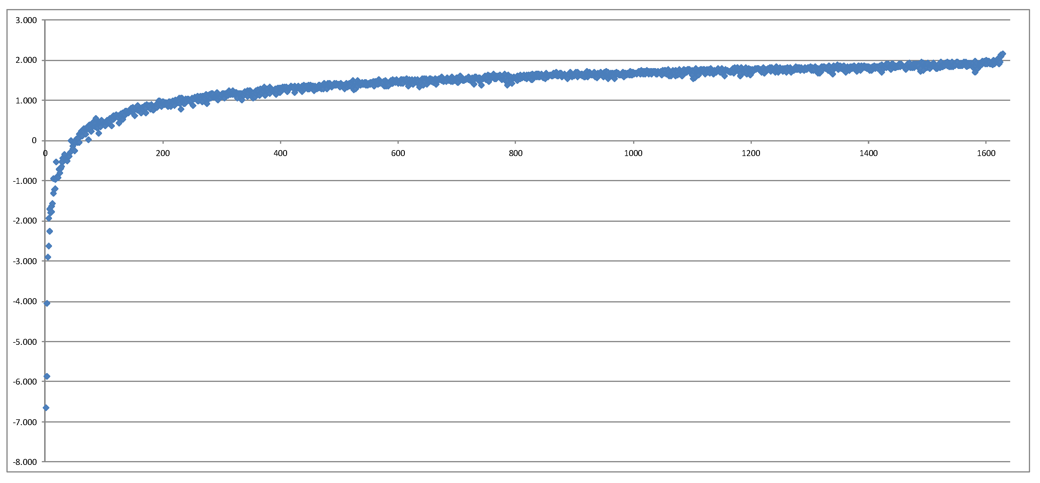
Table 1.
Risk factors in the CFP model.
| Component | Risk Factor Description |
|---|---|
| Risk-free interest rates movement | |
| Change in interest rate volatility | |
| Change in equity volatility | |
| Shock on volatility adjustment (if used by the company) | |
| Credit default | |
| Credit spread widening | |
| Currency exchange rate risk | |
| Shock on equity market value | |
| Shock on property market value | |
| Lapse stress on best estimate assumptions | |
| Mortality catastrophe stress with a one-off increase in mortality | |
| Mortality trend volatility stress | |
| Mortality level stress on best estimate assumptions | |
| Longevity trend volatility stress on best estimate assumptions | |
| Longevity level stress on best estimate assumptions | |
| Morbidity stress on best estimate assumptions | |
| Expenses stress on best estimate assumptions |
Table 2.
Construction sequence of the proxy function in the adaptive algorithm with the final coefficients. Furthermore, AIC and out-of-sample mean squared errors after each iteration.
Table 2.
Construction sequence of the proxy function in the adaptive algorithm with the final coefficients. Furthermore, AIC and out-of-sample mean squared errors after each iteration.
| Iteration | Exponents of Risk Factors | Regression Results | Out-of-Sample MSE | |||||||||||||||
|---|---|---|---|---|---|---|---|---|---|---|---|---|---|---|---|---|---|---|
| AIC | (1) | (2) | ||||||||||||||||
| 0 | 0 | 0 | 0 | 0 | 0 | 0 | 0 | 0 | 0 | 0 | 0 | 0 | 0 | 0 | 8048.89 | 405,919.54 | 279,972.87 | 41,918.48 |
| 1 | 0 | 0 | 0 | 0 | 0 | 0 | 0 | 1 | 0 | 0 | 0 | 0 | 0 | 0 | 5796.16 | 347,121.57 | 22,744.22 | 32,479.31 |
| 2 | 0 | 0 | 0 | 0 | 0 | 1 | 0 | 0 | 0 | 0 | 0 | 0 | 0 | 0 | 80.08 | 342,819.19 | 9863.42 | 5112.25 |
| 3 | 1 | 0 | 0 | 0 | 0 | 0 | 0 | 0 | 0 | 0 | 0 | 0 | 0 | 0 | −28.03 | 337,759.88 | 4048.53 | 4413.39 |
| 4 | 0 | 1 | 0 | 0 | 0 | 0 | 0 | 0 | 0 | 0 | 0 | 0 | 0 | 0 | 26.61 | 336,372.65 | 3003.24 | 4339.50 |
| 5 | 0 | 0 | 0 | 1 | 0 | 0 | 0 | 0 | 0 | 0 | 0 | 0 | 0 | 0 | 108.73 | 335,245.70 | 2534.24 | 4329.35 |
| 6 | 0 | 0 | 0 | 0 | 0 | 0 | 0 | 0 | 0 | 0 | 0 | 1 | 0 | 0 | 22.68 | 334,903.08 | 2334.00 | 4314.37 |
| 7 | 0 | 0 | 0 | 1 | 0 | 0 | 0 | 1 | 0 | 0 | 0 | 0 | 0 | 0 | −614.79 | 334,579.21 | 2257.41 | 4308.28 |
| 8 | 0 | 0 | 0 | 2 | 0 | 0 | 0 | 0 | 0 | 0 | 0 | 0 | 0 | 0 | 297.50 | 334,299.51 | 1341.89 | 1970.71 |
| 9 | 0 | 0 | 0 | 0 | 0 | 0 | 0 | 0 | 0 | 0 | 1 | 0 | 0 | 0 | 32.93 | 334,043.75 | 1376.76 | 1945.95 |
| 10 | 0 | 0 | 0 | 0 | 0 | 0 | 1 | 0 | 0 | 0 | 0 | 0 | 0 | 0 | 71.60 | 333,840.00 | 1084.23 | 1501.77 |
| 11 | 1 | 0 | 0 | 0 | 0 | 0 | 0 | 1 | 0 | 0 | 0 | 0 | 0 | 0 | 57.32 | 333,769.40 | 1134.52 | 1843.88 |
| 12 | 0 | 0 | 0 | 0 | 0 | 0 | 0 | 2 | 0 | 0 | 0 | 0 | 0 | 0 | 1636.91 | 333,523.57 | 638.87 | 748.50 |
| 13 | 0 | 1 | 0 | 0 | 0 | 0 | 0 | 1 | 0 | 0 | 0 | 0 | 0 | 0 | −58.12 | 333,420.22 | 637.63 | 700.10 |
| 14 | 0 | 1 | 0 | 1 | 0 | 0 | 0 | 0 | 0 | 0 | 0 | 0 | 0 | 0 | 15.67 | 333,367.94 | 645.54 | 699.57 |
| 15 | 0 | 0 | 0 | 0 | 0 | 0 | 0 | 0 | 0 | 1 | 0 | 0 | 0 | 0 | 29.69 | 333,316.80 | 327.84 | 172.71 |
| 16 | 0 | 0 | 0 | 1 | 0 | 0 | 0 | 0 | 0 | 0 | 0 | 1 | 0 | 0 | 42.48 | 333,265.87 | 313.90 | 172.91 |
| 17 | 0 | 0 | 0 | 0 | 0 | 0 | 0 | 0 | 0 | 0 | 0 | 0 | 1 | 0 | 13.64 | 333,222.65 | 321.78 | 169.47 |
| 18 | 0 | 0 | 0 | 0 | 0 | 0 | 0 | 0 | 0 | 0 | 0 | 0 | 0 | 1 | 6.81 | 333,182.38 | 280.15 | 167.30 |
| 19 | 1 | 0 | 0 | 1 | 0 | 0 | 0 | 0 | 0 | 0 | 0 | 0 | 0 | 0 | −5.66 | 333,144.02 | 292.49 | 166.74 |
| 20 | 0 | 0 | 1 | 0 | 0 | 0 | 0 | 0 | 0 | 0 | 0 | 0 | 0 | 0 | −9.91 | 333,118.13 | 285.39 | 167.79 |
| 21 | 0 | 0 | 0 | 2 | 0 | 0 | 0 | 1 | 0 | 0 | 0 | 0 | 0 | 0 | −440.05 | 333,093.91 | 259.30 | 178.81 |
| 22 | 0 | 0 | 0 | 0 | 0 | 1 | 0 | 1 | 0 | 0 | 0 | 0 | 0 | 0 | 36.14 | 333,083.85 | 268.45 | 169.96 |
| 23 | 1 | 0 | 0 | 1 | 0 | 0 | 0 | 1 | 0 | 0 | 0 | 0 | 0 | 0 | −35.76 | 333,074.41 | 256.88 | 166.85 |
| 24 | 1 | 0 | 0 | 0 | 0 | 1 | 0 | 0 | 0 | 0 | 0 | 0 | 0 | 0 | 0.85 | 333,066.67 | 270.83 | 163.39 |
| 25 | 0 | 0 | 0 | 0 | 0 | 0 | 0 | 1 | 0 | 0 | 1 | 0 | 0 | 0 | −82.22 | 333,059.15 | 264.46 | 163.59 |
| 26 | 1 | 0 | 0 | 0 | 0 | 0 | 0 | 0 | 0 | 0 | 1 | 0 | 0 | 0 | −2.32 | 333,047.07 | 248.44 | 163.48 |
| 27 | 1 | 0 | 0 | 0 | 0 | 0 | 0 | 0 | 0 | 0 | 0 | 1 | 0 | 0 | −2.21 | 333,039.92 | 254.61 | 163.62 |
| 28 | 0 | 1 | 0 | 0 | 0 | 0 | 0 | 0 | 0 | 0 | 1 | 0 | 0 | 0 | 3.69 | 333,033.27 | 251.67 | 163.51 |
| 29 | 0 | 1 | 0 | 1 | 0 | 0 | 0 | 1 | 0 | 0 | 0 | 0 | 0 | 0 | −48.47 | 333,026.83 | 259.06 | 163.76 |
| 30 | 0 | 1 | 0 | 0 | 0 | 0 | 0 | 2 | 0 | 0 | 0 | 0 | 0 | 0 | 126.06 | 333,020.64 | 255.68 | 162.53 |
| 31 | 0 | 0 | 0 | 1 | 0 | 1 | 0 | 0 | 0 | 0 | 0 | 0 | 0 | 0 | −20.94 | 333,015.48 | 247.72 | 169.26 |
| 32 | 2 | 0 | 0 | 0 | 0 | 0 | 0 | 0 | 0 | 0 | 0 | 0 | 0 | 0 | −0.30 | 333,010.56 | 282.84 | 264.54 |
| 33 | 2 | 0 | 0 | 1 | 0 | 0 | 0 | 0 | 0 | 0 | 0 | 0 | 0 | 0 | −0.98 | 333,001.42 | 290.84 | 273.88 |
| 34 | 0 | 0 | 0 | 2 | 0 | 0 | 0 | 0 | 0 | 0 | 0 | 1 | 0 | 0 | 51.52 | 332,996.57 | 285.59 | 270.99 |
| 35 | 1 | 0 | 0 | 0 | 0 | 0 | 0 | 2 | 0 | 0 | 0 | 0 | 0 | 0 | −93.15 | 332,991.83 | 299.74 | 269.59 |
| 36 | 0 | 0 | 0 | 1 | 0 | 0 | 0 | 0 | 0 | 0 | 0 | 0 | 0 | 1 | −3.99 | 332,987.49 | 294.01 | 269.92 |
| 37 | 0 | 0 | 0 | 0 | 0 | 0 | 0 | 0 | 0 | 0 | 0 | 2 | 0 | 0 | 9.48 | 332,983.89 | 244.46 | 193.39 |
| 38 | 0 | 0 | 0 | 0 | 0 | 0 | 0 | 0 | 0 | 0 | 0 | 3 | 0 | 0 | 17.52 | 332,981.05 | 246.77 | 193.69 |
| 39 | 0 | 0 | 0 | 0 | 0 | 0 | 0 | 1 | 0 | 0 | 0 | 1 | 0 | 0 | −42.29 | 332,978.40 | 252.84 | 193.19 |
| 40 | 0 | 0 | 0 | 3 | 0 | 0 | 0 | 0 | 0 | 0 | 0 | 0 | 0 | 0 | 76.70 | 332,975.77 | 239.20 | 186.54 |
| 41 | 0 | 0 | 0 | 4 | 0 | 0 | 0 | 0 | 0 | 0 | 0 | 0 | 0 | 0 | −279.08 | 332,971.77 | 203.89 | 133.62 |
| 42 | 0 | 1 | 0 | 0 | 0 | 0 | 0 | 0 | 0 | 0 | 0 | 1 | 0 | 0 | 2.57 | 332,969.67 | 208.28 | 133.57 |
| 43 | 0 | 0 | 0 | 0 | 0 | 2 | 0 | 0 | 0 | 0 | 0 | 0 | 0 | 0 | −0.62 | 332,967.85 | 218.11 | 146.76 |
| 44 | 0 | 0 | 0 | 1 | 0 | 2 | 0 | 0 | 0 | 0 | 0 | 0 | 0 | 0 | 4.71 | 332,965.46 | 210.39 | 148.32 |
| 45 | 0 | 0 | 0 | 0 | 0 | 0 | 0 | 0 | 0 | 1 | 0 | 0 | 0 | 1 | 13.36 | 332,963.97 | 208.86 | 148.27 |
| 46 | 0 | 0 | 0 | 1 | 0 | 0 | 0 | 0 | 0 | 0 | 1 | 0 | 0 | 0 | 11.10 | 332,962.49 | 198.29 | 148.32 |
| 47 | 0 | 0 | 2 | 0 | 0 | 0 | 0 | 0 | 0 | 0 | 0 | 0 | 0 | 0 | −5.85 | 332,961.35 | 226.05 | 193.90 |
| 48 | 0 | 0 | 1 | 0 | 0 | 0 | 0 | 0 | 0 | 0 | 0 | 0 | 0 | 1 | 5.69 | 332,960.33 | 222.46 | 193.81 |
| 49 | 0 | 0 | 0 | 0 | 0 | 0 | 0 | 1 | 0 | 1 | 0 | 0 | 0 | 0 | −56.01 | 332,959.53 | 207.33 | 198.33 |
| 50 | 0 | 0 | 0 | 0 | 0 | 0 | 1 | 1 | 0 | 0 | 0 | 0 | 0 | 0 | 70.44 | 332,958.77 | 209.11 | 197.42 |
| 51 | 0 | 0 | 0 | 0 | 0 | 0 | 0 | 3 | 0 | 0 | 0 | 0 | 0 | 0 | 1390.37 | 332,958.18 | 217.77 | 203.07 |
| 52 | 1 | 0 | 0 | 1 | 0 | 1 | 0 | 0 | 0 | 0 | 0 | 0 | 0 | 0 | −1.06 | 332,957.82 | 219.21 | 203.00 |
| 53 | 0 | 0 | 0 | 2 | 0 | 1 | 0 | 0 | 0 | 0 | 0 | 0 | 0 | 0 | −64.50 | 332,957.51 | 192.10 | 159.88 |
| 54 | 0 | 0 | 0 | 2 | 0 | 2 | 0 | 0 | 0 | 0 | 0 | 0 | 0 | 0 | 17.64 | 332,953.46 | 165.97 | 143.94 |
| 55 | 0 | 0 | 0 | 1 | 0 | 0 | 0 | 0 | 0 | 1 | 0 | 0 | 0 | 0 | 17.25 | 332,953.31 | 169.81 | 137.14 |
| 56 | 0 | 0 | 0 | 1 | 0 | 0 | 0 | 0 | 0 | 1 | 0 | 0 | 0 | 1 | 37.24 | 332,951.99 | 172.65 | 137.00 |
| 57 | 0 | 1 | 0 | 0 | 0 | 0 | 0 | 0 | 0 | 0 | 0 | 0 | 1 | 0 | 2.00 | 332,951.87 | 172.90 | 137.59 |
| 58 | 0 | 0 | 0 | 0 | 0 | 0 | 0 | 1 | 0 | 0 | 0 | 0 | 1 | 0 | −26.38 | 332,951.38 | 171.80 | 137.55 |
| 59 | 0 | 0 | 0 | 0 | 0 | 1 | 1 | 0 | 0 | 0 | 0 | 0 | 0 | 0 | 6.21 | 332,951.14 | 182.94 | 149.27 |
| 60 | 0 | 0 | 0 | 1 | 0 | 0 | 0 | 1 | 0 | 0 | 0 | 1 | 0 | 0 | −66.58 | 332,951.14 | 182.17 | 148.10 |
© 2018 by the authors. Licensee MDPI, Basel, Switzerland. This article is an open access article distributed under the terms and conditions of the Creative Commons Attribution (CC BY) license (http://creativecommons.org/licenses/by/4.0/).
Share and Cite
MDPI and ACS Style
Krah, A.-S.; Nikolić, Z.; Korn, R. A Least-Squares Monte Carlo Framework in Proxy Modeling of Life Insurance Companies. Risks 2018, 6, 62. https://doi.org/10.3390/risks6020062
AMA Style
Krah A-S, Nikolić Z, Korn R. A Least-Squares Monte Carlo Framework in Proxy Modeling of Life Insurance Companies. Risks. 2018; 6(2):62. https://doi.org/10.3390/risks6020062
Chicago/Turabian StyleKrah, Anne-Sophie, Zoran Nikolić, and Ralf Korn. 2018. "A Least-Squares Monte Carlo Framework in Proxy Modeling of Life Insurance Companies" Risks 6, no. 2: 62. https://doi.org/10.3390/risks6020062
Note that from the first issue of 2016, this journal uses article numbers instead of page numbers. See further details here.