Hedging and Cash Flows in the Presence of Taxes and Expenses in Life and Pension Insurance

Abstract

In investment and insurance contracts, certain stipulated payments may depend on the hedging strategy. We study the problem of calculation, hedging and valuation of such cash flows, by considering a payment process in a setup with taxes and investment costs that are functions of the investment returns or the current value of the hedging strategy. We determine the market value of the combined liability and decompose the value into the tax part, the investment cost part and the benefit part, and we determine the associated hedging strategies. Moreover, we identify the expected future tax payments and investment cost cash flows. Our results show that the current Danish insurance accounting practice for taxes is in general conservative, when considered in an idealized setting with symmetric and continuously-paid taxes. Finally, we consider the special case of affine interest rates, where explicit results can be obtained, and study some numerical results.

1. Introduction

Under the Solvency 2 regulations, insurance companies should take into consideration all payments related to an insurance contract, when determining the so-called technical provisions, including taxes and expenses; see, e.g., the Solvency 2 regulation EIOPA (2015) and the Solvency 2 directive EIOPA (2009). Thus, when facing the problem of market consistent valuation of an insurance contract under Solvency 2, the insurance company needs to include explicit modeling of the future expenses and taxes. However, under some tax regimes, the taxes are linked to the returns on the underlying investment strategy, which then needs to be included for the valuation of the total liabilities. If the expenses are also linked to the value of the investment strategy, then this also enters in the valuation in a non-trivial manner.

In this paper, we study the problem of the valuation and hedging of insurance and investment payment processes in a framework that takes explicitly into consideration payments that depend on the associated hedging strategy, through the investment returns and the current value of the investment strategy. Examples are investment expenses and taxes on investment returns. This situation differs from the traditional problem of valuating and hedging a payment process that depends on the financial market and perhaps some additional risk, but where the choice of hedging strategy does not affect the payment process itself.

Our results are related to, and shed new light on, current Danish insurance accounting practice. Under the Danish insurance regulation, the insurance companies pay taxes yearly, which are essentially determined as a fraction $\gamma$ (=15.3%) of the returns on the investments. In practice, Danish companies typically account for this tax by calculating the market value of their liabilities using a tax-reduced forward rate curve, where the forward rate is reduced by the tax rate of 15.3%. We show in the paper that this is a conservative upper bound for the true value of the liability including the future tax payments in an idealized setting, where (positive and negative) tax is paid continuously. In models with stochastic interest, the theoretical value will be strictly smaller than this upper bound typically used in practice.

We consider a traditional complete and arbitrage-free dynamic financial market in a continuous time setting, where all payment processes can be hedged and priced uniquely; see, e.g., Björk (2004) for an introduction to financial mathematics and Møller (2001) and Møller and Steffensen (2007) for applications in insurance. Thus, for each payment process, there exists a self-financing hedging strategy that replicates the payment process, and the unique no-arbitrage price can be determined as the expected value of the discounted payments, calculated under a so-called equivalent martingale measure.

We then extend the model by introducing two additional types of payments that are closely related to the choice of hedging strategy and the current value of the investment strategy associated with an insurance payment process. We are focusing on an insurance company that is interested in hedging an insurance liability as given by an insurance payment process. The company allocates a portfolio and a certain investment strategy for the purpose of hedging this liability. This hedging scheme leads to two additional liabilities, the investments costs and taxes on the returns generated by the investment strategy.

The investment costs are assumed to incur continuously at a rate, which is proportional to the current value of the current investment portfolio. Hence, the size of the current expenses is directly linked to the current value of the investment portfolio. The taxes are also assumed to be incurred continuously and are calculated as a fixed fraction of the current investment returns. In this setting, we study the problem of valuation and hedging of the combined liability consisting of the original insurance payment process, the future investment costs and the future taxes. We show that if the original market (without taxes and expenses) is complete and arbitrage free, we are able to price and hedge payment processes that depend on the hedging strategy via taxes and expenses. Moreover, we decompose the value of the replicating strategy into the value of the future insurance payments and the combined value of expenses and taxes. Whereas there exists a vast literature on the problem of hedging under transactions costs (see, e.g., Leland 1985; Soner et al. 1995; Damgaard 2003; Damgaard 2006), the recent literature on tax-adjustment of yield curves seems more limited; older literature includes McCulloch (1975) and the references therein.

The paper is organized as follows. In Section 2, we introduce the underlying financial market without taxes and expenses. In Section 3, the traditional setting is extended by allowing for continuously-paid taxes and expenses that are directly linked to current returns from the underlying investment strategy and to its current value. In Section 4, we study the celebrated case of the one-dimensional affine term structure model driven by a Brownian motion, which encompasses both the Vasicek and the Cox–Ingersoll–Ross (CIR) models; see, e.g., Filipovic (2009) and Björk (2004). Within this model with two investment possibilities, a zero coupon bond expiring at T and the savings account, we study a simple insurance payment process, which includes a fixed payment of one unit at a fixed time T. For this simple insurance payment process, we derive explicit formulas for the replicating strategy in the presence of taxes and expenses. For the Vasicek model, the optimal strategy consists of investing in the underlying zero-coupon bond with maturity T only and adjusting this amount continuously to finance taxes and expenses; for the CIR-model, the optimal strategy is a dynamic strategy in the zero-coupon bond with a negative position in the savings account. A numerical example is included in Section 5.

2. The Complete Financial Market: A Review

This section contains a review of some classic results from the literature on financial mathematics on pricing and hedging in complete markets without taxes and expenses; for unexplained terminology, see, e.g., Møller and Steffensen (2007); Björk (2004) and the references therein. The presentation focuses on well-known concepts that are essential for the introduction of taxes and expenses in Section 3. For example, we recall how the discounted and the undiscounted price processes are related, and we recall the definition of self-financing strategies and attainability in the presence of a payment process.

Consider a general and complete financial market with a fixed finite time horizon T. All processes are assumed to be adapted and defined on a probability space $(\Omega ,\mathcal{F},P)$ equipped with a filtration ${\left(\mathcal{F}\left(t\right)\right)}_{t\in [0,T]}$.

2.1. Traded Assets

The financial market is assumed to consist of a savings account $S_0={\left(S_0\left(t\right)\right)}_{0\le t\le T}$ and d additional assets with price processes $(S_1,\dots ,S_d)$. Investments in the savings account are accumulated continuously with a (stochastic) short rate $r\left(t\right)$, such that the value at time t of a unit invested in the savings account at Time 0 is:

$$\begin{array}{c}{S}_0\left(t\right)=e^{{\int }_0^{t}r\left(u\right)\mathrm{d}u}.\hfill \end{array}$$

(1)

We introduce the discounted asset price processes $(S_0^{*},S_1^{*},\dots ,S_d^{*})$ by using the savings account $S_0$ as numeraire, i.e., $S_i^{*}\left(t\right)=S_i\left(t\right)/S_0\left(t\right)$. In particular, this means that $S_0^{*}\left(t\right)=1$ for all $t\in [0,T]$. We assume that there exists an equivalent measure Q, such that the discounted prices processes $S_i^{*}$ are Q-martingales. The measure Q is also called an equivalent martingale measure; see, e.g., Björk (2004).

By using that:

$$\begin{array}{c}\mathrm{d}{\left(S_0\left(t\right)\right)}^{-1}=-r\left(t\right){\left(S_0\left(t\right)\right)}^{-1}\mathrm{d}t,\hfill \end{array}$$

(2)

we see that the dynamics for the discounted price processes are given by:

$$\begin{array}{c}\mathrm{d}{S}_j^{*}\left(t\right)={\left(S_0\left(t\right)\right)}^{-1}\mathrm{d}{S}_j\left(t\right)-r\left(t\right)S_j^{*}\left(t\right)\mathrm{d}t,\hfill \end{array}$$

which implies that:

$$\begin{array}{c}{\left(S_0\left(t\right)\right)}^{-1}\mathrm{d}{S}_j\left(t\right)=\mathrm{d}{S}_j^{*}\left(t\right)+r\left(t\right)S_j^{*}\left(t\right)\mathrm{d}t.\hfill \end{array}$$

(3)

Thus, if we interpret $\mathrm{d}{S}_j\left(t\right)$ as the change in the price process in a small interval, we see from (3) that if we discount this amount using the short rate r, this discounted amount is equal to the change in the discounted price process, plus interest on the discounted price process.

For example, the financial market could be a so-called Black–Scholes market consisting of a savings account with a fixed, deterministic short rate r and one risky asset, a stock, with a price process that is defined as a geometric Brownian motion. Alternatively, we could consider a so-called bond market model with stochastic interest, which consists of a savings account and a zero coupon bond expiring at time T.

2.2. Payment Processes

Consider now a payment process A, which is an adapted càdlàg process stipulating the payments associated with a given contract. Here, $A\left(t\right)$ represents the accumulated payments during $[0,t]$, and $\mathrm{d}A\left(t\right)$ can be interpreted as the payments occurring during the time interval $(t,t+\mathrm{d}t)$. The payment process may specify a payment $A\left(0\right)$ at Time 0, and we take $A(0-)=0$. Similarly, we introduce the discounted payment process $A^{*}$ defined by $A^{*}(0-)=0$ and:

$$\begin{array}{c}\mathrm{d}{A}^{*}\left(t\right)={\left(S_0\left(t\right)\right)}^{-1}\mathrm{d}A\left(t\right)=e^{-{\int }_0^{t}r\left(u\right)\mathrm{d}u}\mathrm{d}A\left(t\right).\hfill \end{array}$$

(4)

Thus, $A^{*}\left(t\right)$ is the discounted payments during $[0,t]$, and it is given by:

$$\begin{array}{c}{A}^{*}\left(t\right)={\int }_{[0,t]}{e}^{-{\int }_0^{s}r\left(u\right)\mathrm{d}u}\mathrm{d}A\left(s\right).\hfill \end{array}$$

(5)

We view the payment process A as a liability, and we are interested in the problem of pricing and hedging the contract associated with this payment process. A fundamental and well-known result on complete (and arbitrage free) markets is that there exists a unique arbitrage-free price for any contract, which can be calculated as the expected value of the total discounted payments, where the expected value is calculated with respect to the equivalent martingale measure Q; see, e.g., Björk (2004). This unique price, which is also called the no-arbitrage price for the liability, is exactly the amount needed in order to generate the payments prescribed by the payment process. We include this result in Theorem 1 below.

2.3. Trading and the Value Process with Payment Processes

A trading strategy is an adapted and sufficiently integrable $(d+1)$-dimensional process $h=(h_0,h_1,\dots ,h_d)$, which prescribes the number of units invested in the savings account and in each of the additional d assets (more precisely, we require that $h_0$ is adapted and that $h_1,\dots ,h_d$ are predictable).

We define the (undiscounted) value process associated with the strategy h as:

$$\begin{array}{c}V(h,t)=\sum _{j=0}^d{h}_j\left(t\right)S_j\left(t\right).\hfill \end{array}$$

(6)

Thus, the value at time t is calculated by simply adding the values of the investments in each of the underlying assets, which are determined by multiplying the number $h_j\left(t\right)$ of units of each asset j by the value $S_j\left(t\right)$ of the asset.

We now address the problem of pricing and hedging the payment process A. The main idea is as follows: Can we find an initial amount (the price) to be invested at Time 0 and then design a so-called dynamic investment strategy that leads to total investment returns during the period $[0,t]$, which (together with the initial investment) is exactly equal to the payments $A\left(T\right)$ during $[0,T]$. The amount $V(h,0-)$ to be invested at Time 0 is given as:

$$\begin{array}{c}V(h,0-)=\sum _{j=0}^d{h}_j(0-)S_j\left(0\right),\hfill \end{array}$$

where we have assumed that $S_j(0-)=S_j\left(0\right)$, and we think of $V(h,t)$ as the value of the portfolio h at time t, after we have paid the liabilities $A\left(t\right)$ during $[0,t]$. We are focusing on so-called self-financing strategies, which are investment strategies, which only require a capital injection at Time 0 (before the potential payment $A\left(0\right)$); after this time point, we are neither adding nor withdrawing capital from our investments, but we reduce (or increase) the value with the current payments described by the payment process A. This means that all changes in the value process are either generated by trading gains or are a result of the payments associated with the payment process. This is made precise in the following definition.

Definition 1.

A strategy h is said to be self-financing for the payment process A if the value process defined by (6) satisfies:

$$\begin{array}{c}V(h,t)=V(h,0-)+\sum _{j=0}^d{\int }_{[0,t]}{h}_j\left(u\right)\mathrm{d}{S}_j\left(u\right)-A\left(t\right),\hfill \end{array}$$

(7)

for all $t\in [0,T]$. If, moreover, $V(h,T)=0$, then h is said to replicate A.

We can also write (7) on the differential form:

$$\begin{array}{c}\mathrm{d}V(h,t)=\sum _{j=0}^d{h}_j\left(t\right)\mathrm{d}{S}_j\left(t\right)-\mathrm{d}A\left(t\right).\hfill \end{array}$$

(8)

Here, the terms $h_j\left(t\right)\mathrm{d}{S}_j\left(t\right)$ are the trading gains from asset j, which are calculated as the number of units $h_j\left(t\right)$ multiplied by the change $\mathrm{d}{S}_j\left(t\right)$ in the value of one unit of asset j. Thus, (7) and, equivalently, (8) state that all changes in the value process of a self-financing strategy are generated by either trading gains $h_j\left(t\right)\mathrm{d}{S}_j\left(t\right)$ or payments $\mathrm{d}A\left(t\right)$.

We can identify the total trading gains associated with the strategy h during $[0,T]$ as:

$$\begin{array}{c}\sum _{j=0}^d{\int }_{[0,T]}{h}_j\left(u\right)\mathrm{d}{S}_j\left(u\right).\hfill \end{array}$$

(9)

The following definition introduces the concepts of attainability and completeness.

Definition 2.

A payment process A is said to be attainable if there exists a self-financing strategy h, such that $V(h,T)=0$ P-a.s., i.e.,

$$\begin{array}{c}A\left(T\right)=V(h,0-)+\sum _{j=0}^d{\int }_{[0,T]}{h}_j\left(u\right)\mathrm{d}{S}_j\left(u\right).\hfill \end{array}$$

(10)

The financial market is said to be complete if all payment processes are attainable.

In this paper, we assume that the financial market is complete, which means that all payment processes can be replicated in the sense of (10) by using a self-financing strategy h; see Møller (2001) for more details. The interpretation of (10) is that the total payments $A\left(T\right)$ during $[0,T]$ can in fact be represented as the initial value $V(h,0)$ of the investment strategy added to the trading gains represented by the stochastic integrals with respect to the traded price processes. We note that this equation is not generally valid, nor needed at other times $t<T$.

It is useful to work directly with the discounted value process defined by:

$$\begin{array}{c}{V}^{*}(h,t)={\left(S_0\left(t\right)\right)}^{-1}V(h,t).\hfill \end{array}$$

(11)

By using the definition (7) of a self-financing strategy and the relation (3) between the undiscounted and discounted price processes, we see that:

$$\begin{array}{cc}\mathrm{d}{V}^{*}(h,t)\hfill & ={\left(S_0\left(t\right)\right)}^{-1}\mathrm{d}V(h,t)+V(h,t)\mathrm{d}\left({\left(S_0\left(t\right)\right)}^{-1}\right)\hfill \\ & ={\left(S_0\left(t\right)\right)}^{-1}\left(\sum _{j=0}^d{h}_j\left(t\right)\mathrm{d}{S}_j\left(t\right)-\mathrm{d}A\left(t\right)\right)-r\left(t\right)V^{*}(h,t)\mathrm{d}t\hfill \\ & =\sum _{j=0}^d{h}_j\left(t\right)\left(\mathrm{d}{S}_j^{*}\left(t\right)+r\left(t\right)S_j^{*}\left(t\right)\mathrm{d}t\right)-\mathrm{d}{A}^{*}\left(t\right)-r\left(t\right)V^{*}(h,t)\mathrm{d}t\hfill \\ & =\sum _{j=1}^d{h}_j\left(t\right)\mathrm{d}{S}_j^{*}\left(t\right)-\mathrm{d}{A}^{*}\left(t\right).\hfill \end{array}$$

Here, the first equality follows by (11); the second equality follows from (2) and (8); and the third equality is obtained by using (3) and the definition of the discounted payment process. Finally, in the last equality, we have used that $S_0^{*}\left(t\right)=1$, such that $\mathrm{d}{S}_0^{*}\left(t\right)=0$, and the definition (6) for $V(h,t)$.

Thus, we can rewrite the definition of a self-financing strategy in terms of the discounted quantities. It follows that the discounted version of (7) is given by:

$$\begin{array}{c}{V}^{*}(h,t)=V^{*}(h,0-)+\sum _{j=1}^d{\int }_{[0,t]}{h}_j\left(u\right)\mathrm{d}{S}_j^{*}\left(u\right)-A^{*}\left(t\right),\hfill \end{array}$$

(12)

for any self-financing strategy h.

It is not difficult to see that a self-financing strategy h for A is easily constructed if we do not require that the strategy replicates A. Indeed, for any choice of processes $h_1,\dots ,h_d$, we can choose $h_0$ such that the strategy $h=(h_0,h_1,\dots ,h_d)$ is self-financing for A. Since the discounted value process is defined by (11), the condition (12) directly shows how $h_0\left(t\right)$ must be defined. This is formulated as a lemma below.

Lemma 1.

For any $(h_1,\dots ,h_d)$ define a strategy h via $h=(h_0,h_1,\dots ,h_d)$, where:

$$\begin{array}{c}{h}_0\left(t\right)=V^{*}(h,0-)+\sum _{j=1}^d{\int }_{[0,t]}{h}_j\left(u\right)\mathrm{d}{S}_j^{*}\left(u\right)-A^{*}\left(t\right)-\sum _{j=1}^d{h}_j\left(t\right)S_j^{*}\left(t\right).\hfill \end{array}$$

(13)

Then, h is self-financing for A.

For example, one self-financing strategy for A can be constructed as $h_j\left(t\right)=0$, $j=1,\dots ,d$, and:

$$\begin{array}{c}{h}_0\left(t\right)=V^{*}(h,0-)-A^{*}\left(t\right).\hfill \end{array}$$

In this case, the insurer only invests in the savings account and finances all payments by reducing the deposit in the savings account. Such a strategy will rarely replicate A.

If A is attainable, then there exists a self-financing strategy h that replicates A, such that $V(h,T)=0$ and, equivalently, $V^{*}(h,T)=0$. For this particular choice of strategy h, (12) implies that:

$$\begin{array}{c}{A}^{*}\left(T\right)=V^{*}(h,0-)+\sum _{j=1}^d{\int }_{[0,T]}{h}_j\left(u\right)\mathrm{d}{S}_j^{*}\left(u\right).\hfill \end{array}$$

(14)

Now, define a Q-martingale ${\mathcal{V}}^{A^{*}}\left(t\right)$ by:

$$\begin{array}{c}{\mathcal{V}}^{A^{*}}\left(t\right)=E^Q\left[\left.A^{*}\left(T\right)\right|\mathcal{F}\left(t\right)\right]=E^Q\left[\left.{\int }_{[0,T]}{e}^{-{\int }_0^{s}r\left(u\right)\mathrm{d}u}\mathrm{d}A\left(s\right)\right|\mathcal{F}\left(t\right)\right].\hfill \end{array}$$

(15)

In particular, ${\mathcal{V}}^{A^{*}}(0-)=E^Q\left[A^{*}\left(T\right)\right]$. In the literature, the process (15) is also called the intrinsic value process; see, e.g., Møller (2001). Since the discounted price processes are Q-martingales, it follows from (14) that:

$$\begin{array}{c}{\mathcal{V}}^{A^{*}}\left(t\right)=V^{*}(h,0-)+\sum _{j=1}^d{\int }_{[0,t]}{h}_j\left(u\right)\mathrm{d}{S}_j^{*}\left(u\right),\hfill \end{array}$$

(16)

where we use that h and $S_j^{*}$ are adapted. If we combine this result with (12), we see that we have in fact shown that the discounted value $V^{*}(h,t)$ of the replicating and self-financing strategy at time t is given by:

$$\begin{array}{c}{V}^{*}(h,t)={\mathcal{V}}^{A^{*}}\left(t\right)-A^{*}\left(t\right)=E^Q\left[\left.A^{*}\left(T\right)-A^{*}\left(t\right)\right|\mathcal{F}\left(t\right)\right],\hfill \end{array}$$

(17)

where the second equality follows from the definition of ${\mathcal{V}}^{A^{*}}$ and the $\mathcal{F}\left(t\right)$-measurability of $A^{*}\left(t\right)$. Thus, the value $V^{*}(h,t)$ at time t is exactly given by the conditional expected value of the future discounted payments $A^{*}\left(T\right)-A^{*}\left(t\right)$; see (17). In (15), we have inserted the definition (5) of the discounted payment process in the second equality. This equation underlines that the intrinsic value process is the conditional expected value of all discounted (future and past) payments, where all payments are discounted to Time 0. Hence, the intrinsic value process decomposes into two parts, one part with the past payments and one part with the conditional expected value of all future discounted payments. The second part resembles a traditional discounted prospective reserve in life and pension insurance.

One can use these results to construct a self-financing strategy, which replicates a payment process A by combining (13) and (17). Lemma 1 shows via (13) how one can determine the discounted deposit $h_0$ in the savings account, given the other components of the strategy $h_1,\dots ,h_d$, in order to ensure that the strategy is self-financing. Note, however, that this will not in general lead to a strategy that replicates A in the sense of Definition 1. The strategy will only replicate the payment process A, if $h_1,\dots ,h_d$ are chosen in accordance with (16) or, equivalently, if (14) is satisfied. To see this, we note that if we can determine processes $h_j$, $j=1,\dots ,d$, such that (14) is satisfied, the liability defined by the payment process A can indeed be replicated by following a self-financing investment strategy with a discounted value process given by (12). This is obtained by choosing $h_0\left(t\right)$ according to (13) in Lemma 1, and using (16), we can rewrite this as,

$$\begin{array}{cc}{h}_0\left(t\right)\hfill & =V^{*}(h,0-)+\sum _{j=1}^d{\int }_{[0,t]}{h}_j\left(u\right)\mathrm{d}{S}_j^{*}\left(u\right)-A^{*}\left(t\right)-\sum _{j=1}^d{h}_j\left(t\right)S_j^{*}\left(t\right)\hfill \\ & ={\mathcal{V}}^{A^{*}}\left(t\right)-A^{*}\left(t\right)-\sum _{j=1}^d{h}_j\left(t\right)S_j^{*}\left(t\right).\hfill \end{array}$$

We have now shown the following result.

Theorem 1.

Consider an attainable payment process A. The unique arbitrage-free price for A is given by $E^Q\left[A^{*}\left(T\right)\right]$.

The payment process can be replicated by a self-financing strategy h, where the components $(h_1\left(t\right),\dots ,h_d\left(t\right))$ are determined from (14) and where $h_0\left(t\right)$ is given by:

$$\begin{array}{c}{h}_0\left(t\right)={\mathcal{V}}^{A^{*}}\left(t\right)-A^{*}\left(t\right)-\sum _{j=1}^d{h}_j\left(t\right)S_j^{*}\left(t\right).\hfill \end{array}$$

(18)

Note that Equation (18) in Theorem 1 and Equation (13) in Lemma 1 both provide characterizations of the discounted amount deposited in the savings account. The difference between the two equations is that Lemma 1 does not assume that the strategy replicates the payment process.

2.4. A Short Overview of the Review on Complete Financial Markets

In Section 2, we have studied payment processes, which are not affected by the choice of investment strategy. For this situation, we have reviewed some fundamental results on the valuation and hedging of payment processes in a complete market, where all payment processes can be perfectly hedged via a self-financing strategy. In particular, we introduced the so-called intrinsic value process defined by (15) and demonstrated how this process can be used in the complete case for determining a self-financing strategy, which replicates a given payment process.

3. Hedging with Taxes and Expenses

We extend the setting from the previous section by allowing for continuously-paid expenses and continuously-paid taxes on returns. We study an insurance company facing a liability payment process $A^{\mathrm{b}}$; the superscript $\mathrm{b}$ is an abbreviation for benefits (possibly reduced by premiums). The insurance company invests in the assets in the financial market described in Section 2.1. We introduce the relevant payment processes describing the additional liabilities associated with the expenses and taxes and define self-financing strategies in this context.

Now, consider an investment strategy $\tilde{h}$ with value process $V(\tilde{h},t)$ defined by (6). In addition to the liability payment process $A^{\mathrm{b}}$, the company has two additional liabilities that are affected by the investments. The company is assumed to continuously pay taxes that are determined as a fraction $\gamma <1$ of all returns (positive and negative) from the investment strategy $\tilde{h}$ and expenses determined as a fraction, $\delta$, of the value of the strategy. Thus, the taxes are defined by the tax payment process $A^{\mathrm{t}}(\tilde{h})$ with:

$$\begin{array}{c}\mathrm{d}{A}^{\mathrm{t}}(\tilde{h},t)=\sum _{j=0}^d\gamma {\tilde{h}}_j\left(t\right)\mathrm{d}{S}_j\left(t\right),\hfill \end{array}$$

(19)

and the expenses are defined by the expense payment process $A^{\mathrm{e}}(\tilde{h})$ with:

$$\begin{array}{c}\mathrm{d}{A}^{\mathrm{e}}(\tilde{h},t)=\delta V(\tilde{h},t)\mathrm{d}t.\hfill \end{array}$$

(20)

Note that these two payment processes depend on the choice of investment strategy $\tilde{h}$ via the returns on the investments and the current value of the investment strategy. This is a crucial difference from the setting in the previous sections, where the liability payment process was unaffected by the choice of investment strategy. When we determine a self-financing strategy for the insurance payment process $A^{\mathrm{b}}$, we need to take into consideration the fact that the strategy also affects the additional payment processes $A^{\mathrm{t}}$ and $A^{\mathrm{e}}$.

It is natural to extend the definition of a self-financing strategy from the previous section to the following definition.

Definition 3.

A strategy $\tilde{h}$ is said to be self-financing for the insurance payment process $A^{\mathrm{b}}$ in the presence of taxes and expenses if the value process $V(\tilde{h},t)$ is given by:

$$\begin{array}{c}V(\tilde{h},t)=V(\tilde{h},0-)+\sum _{j=0}^d{\int }_{[0,t]}{\tilde{h}}_j\left(u\right)\mathrm{d}{S}_j\left(u\right)-A^{\mathrm{b}}\left(t\right)-A^{\mathrm{t}}(\tilde{h},t)-A^{\mathrm{e}}(\tilde{h},t).\hfill \end{array}$$

(21)

If, moreover $V(\tilde{h},T)=0$, then the strategy $\tilde{h}$ is said to replicate the insurance liability process $A^{\mathrm{b}}$ in the presence of taxes and expenses.

The interpretation of (21) is as follows: If $\tilde{h}$ is self-financing, the value of the portfolio at time t is defined as the initial value $V(\tilde{h},0-)$ before any payments have taken place, added trading gains and reduced by payments prescribed by $A^{\mathrm{b}}$, taxes and expenses.

By inserting the dynamics for the tax and expense payment processes in (21), we see that this definition can alternatively be written in the form:

$$\begin{array}{c}V(\tilde{h},t)=V(\tilde{h},0-)+\sum _{j=0}^d{\int }_{[0,t]}(1-\gamma ){\tilde{h}}_j(u)\mathrm{d}{S}_j(u)-A^{\mathrm{b}}(t)-{\int }_{[0,t]}\delta V(\tilde{h},u)\mathrm{d}u.\hfill \end{array}$$

(22)

We are interested in finding an investment strategy $\tilde{h}$ that replicates the three liability payment processes in order to obtain an investment strategy and in finding the value of the initial investment $V(\tilde{h},0-)$ needed in order to replicate the liability, i.e., the price of the liability. According to this definition, we need to determine $\tilde{h}$ such that $V(\tilde{h},T)=0$, i.e.,

$$\begin{array}{c}{A}^{\mathrm{b}}(T)+A^{\mathrm{e}}(\tilde{h},T)=V(\tilde{h},0-)+\sum _{j=0}^d{\int }_{[0,T]}(1-\gamma ){\tilde{h}}_j(u)\mathrm{d}{S}_j(u).\hfill \end{array}$$

(23)

This seems more complicated than the situation (10) without taxes and expenses, since $A^{\mathrm{e}}(\tilde{h},T)$ depends on $\tilde{h}$ such that $\tilde{h}$ appears on both sides of the equation (23).

The following result for the discounted value process is useful.

Lemma 2.

Consider a strategy $\tilde{h}$. Then, $\tilde{h}$ is a self-financing strategy for the insurance payment process $A^{\mathrm{b}}$ in the presence of taxes and expenses if and only if the discounted value process $V^{*}(\tilde{h},t)$ is given by:

$$\begin{array}{ccc}{V}^{*}(\tilde{h},t)& =& e^{-{\int }_0^t(\gamma r\left(u\right)+\delta )\mathrm{d}u}\left(V^{*}(\tilde{h},0-)+{\int }_{[0,t]}{e}^{{\int }_0^u(\gamma r\left(\tau \right)+\delta )\mathrm{d}\tau }\sum _{j=1}^d{\tilde{h}}_j\left(u\right)(1-\gamma )\mathrm{d}{S}_j^{*}\left(u\right)\right.\hfill \\ -\left.{\int }_{[0,t]}{e}^{-{\int }_0^u((1-\gamma )r\left(\tau \right)-\delta )\mathrm{d}\tau }\mathrm{d}{A}^{\mathrm{b}}\left(u\right)\frac{{}^{}}{{}^{}}\right),\hfill \end{array}$$

(24)

or, equivalently:

$$\begin{array}{cc}\mathrm{d}{V}^{*}(\tilde{h},t)=\hfill & \sum _{j=1}^d(1-\gamma ){\tilde{h}}_j\left(t\right)\mathrm{d}{S}_j^{*}\left(t\right)-(\gamma r\left(t\right)+\delta )V^{*}(\tilde{h},t)\mathrm{d}t-\mathrm{d}{A}^{\mathrm{b},*}\left(t\right).\hfill \end{array}$$

(25)

Proof. 

By differentiating (24), we first see that this coincides with (25). The result now follows directly from the definition of a self-financing strategy and the definition of the discounted value process. By using (3) and the definition of the value process, we see that:

$$\begin{array}{ccc}\mathrm{d}{V}^{*}(\tilde{h},t)\hfill & =& {\left(S_0\left(t\right)\right)}^{-1}\mathrm{d}V(\tilde{h},t)+V(\tilde{h},t)\mathrm{d}\left(S_0{\left(t\right)}^{-1}\right)\hfill \\ & =\hfill & {\left(S_0\left(t\right)\right)}^{-1}\left(\sum _{j=0}^d(1-\gamma ){\tilde{h}}_j\left(t\right)\mathrm{d}{S}_j\left(t\right)-\mathrm{d}{A}^{\mathrm{b}}\left(t\right)-\delta V(\tilde{h},t)\mathrm{d}t\right)-r\left(t\right)V^{*}(\tilde{h},t)\mathrm{d}t\hfill \\ & =\hfill & \sum _{j=1}^d(1-\gamma ){\tilde{h}}_j\left(t\right)\mathrm{d}{S}_j^{*}\left(t\right)-(\gamma r\left(t\right)+\delta )V^{*}(\tilde{h},t)\mathrm{d}t-\mathrm{d}{A}^{\mathrm{b},*}\left(t\right).\hfill \end{array}$$

(26)

In the second equality, we have used (22), since $\tilde{h}$ is assumed to be self-financing for $A^{\mathrm{b}}$ in the presence of expenses and taxes. This completes the proof. ☐

We observe that the expression (24) for the discounted value process in the presence of expenses and taxes is considerably more complicated than the similar expression (12) without taxes and expenses.

Define the tax and expense-adjusted discounted insurance payment process ${\tilde{A}}^{\mathrm{b}}$ by:

$$\begin{array}{c}{\tilde{A}}^{\mathrm{b}}\left(t\right)={\int }_{[0,t]}{e}^{{\int }_0^u(\gamma r\left(s\right)+\delta )\mathrm{d}s}\mathrm{d}{A}^{\mathrm{b},*}\left(u\right)={\int }_{[0,t]}{e}^{-{\int }_0^u((1-\gamma )r\left(s\right)-\delta )\mathrm{d}s}\mathrm{d}{A}^{\mathrm{b}}\left(u\right).\hfill \end{array}$$

(27)

This term appears in (24) and can be interpreted as the total discounted payments during $[0,t]$, appropriately modified for taxes and expenses. Thus, payments occurring at time t are adjusted for taxes $\gamma$ and expenses $\delta$ via the factor $exp\left({\int }_0^t(\gamma r\left(s\right)+\delta )\mathrm{d}s\right)$, as well as interest by the factor $exp(-{\int }_0^{t}r\left(s\right)\mathrm{d}s)$. We note that $\widetilde{A^{\mathrm{b}}}\left(T\right)$ does not depend on the choice of investment strategy.

Note that if ${\tilde{h}}^A$ is self-financing for $A^{\mathrm{b}}$ in the presence of taxes and expenses and replicates $A^{\mathrm{b}}$, such that $V({\tilde{h}}^A,T)=0$, then $V^{*}({\tilde{h}}^A,T)=0$, and Lemma 2 implies that:

$$\begin{array}{c}{\tilde{A}}^{\mathrm{b}}\left(T\right)=V^{*}({\tilde{h}}^A,0-)+{\int }_{[0,T]}\sum _{j=1}^d\left({\tilde{h}}_j^A\left(u\right)(1-\gamma )e^{{\int }_0^u(\gamma r\left(\tau \right)+\delta )\mathrm{d}\tau }\right)\mathrm{d}{S}_j^{*}\left(u\right).\hfill \end{array}$$

(28)

Define a Q-martingale ${\mathcal{V}}^{\tilde{A}}\left(t\right)$ via:

$$\begin{array}{cc}{\mathcal{V}}^{{\tilde{A}}^{\mathrm{b}}}\left(t\right)\hfill & =E^Q\left[\left.{\tilde{A}}^{\mathrm{b}}\left(T\right)\right|\mathcal{F}\left(t\right)\right]\hfill \\ & =V^{*}(h^A,0-)+{\int }_{[0,t]}\sum _{j=1}^d\left({\tilde{h}}_j^A\left(u\right)(1-\gamma )e^{{\int }_0^u(\gamma r\left(\tau \right)+\delta )\mathrm{d}\tau }\right)\mathrm{d}{S}_j^{*}\left(u\right),\hfill \end{array}$$

where we have used (28) in the second equality. We can now use Lemma 2 to conclude that if ${\tilde{h}}^A$ is self-financing and replicates $A^{\mathrm{b}}$ in the presence of taxes and expenses, then (24) implies that:

$$\begin{array}{c}{V}^{*}(h^A,t)=e^{-{\int }_0^t(\gamma r\left(u\right)+\delta )\mathrm{d}u}\left({\mathcal{V}}^{{\tilde{A}}^{\mathrm{b}}}\left(t\right)-{\tilde{A}}^{\mathrm{b}}\left(t\right)\right).\hfill \end{array}$$

(29)

This value can be interpreted as the Q-expectation of the future tax- and expense-adjusted payments $E^Q\left[\left.{\tilde{A}}^{\mathrm{b}}\left(T\right)-{\tilde{A}}^{\mathrm{b}}\left(t\right)\right|\mathcal{F}\left(t\right)\right]$, where the tax and expense adjustment is only for the time period $[t,T]$.

We are now ready to present the following result.

Theorem 2.

Assume that there exists $h^{\circ }$ such that ${\tilde{A}}^{\mathrm{b}}\left(T\right)$ has the representation:

$$\begin{array}{c}{\tilde{A}}^{\mathrm{b}}\left(T\right)=V^{*}(h^{\circ },0-)+{\int }_{[0,T]}\sum _{j=1}^d{h}_j^{\circ }\left(u\right)\mathrm{d}{S}_j^{*}\left(u\right).\hfill \end{array}$$

(30)

Then, $A^{\mathrm{b}}$ is attainable in the presence of taxes and expenses.

Define a strategy ${\tilde{h}}^{A^{\mathrm{b}}}$ via:

$$\begin{array}{c}{\tilde{h}}_j^{A^{\mathrm{b}}}\left(t\right)=\frac{1}{1-\gamma }{e}^{-{\int }_0^t(\gamma r\left(\tau \right)+\delta )\mathrm{d}\tau }{h}_j^{\circ }\left(t\right),\hfill \end{array}$$

(31)

for $j=1,\dots ,d$, and:

$$\begin{array}{c}{\tilde{h}}_0^{A^{\mathrm{b}}}\left(t\right)=e^{-{\int }_0^t(\gamma r\left(\tau \right)+\delta )\mathrm{d}\tau }\left({\mathcal{V}}^{{\tilde{A}}^{\mathrm{b}}}\left(t\right)-{\tilde{A}}^{\mathrm{b}}\left(t\right)\right)-\sum _{j=1}^d{\tilde{h}}_j^{A^{\mathrm{b}}}\left(t\right)S_j^{*}\left(t\right).\hfill \end{array}$$

(32)

Then, ${\tilde{h}}^{A^{\mathrm{b}}}$ is self-financing for $A^{\mathrm{b}}$ in the presence of tax and expenses and ${\tilde{h}}^{A^{\mathrm{b}}}$ replicates $A^{\mathrm{b}}$, i.e., $V^{*}(T,{\tilde{h}}^{A^{\mathrm{b}}})=0$.

Proof. 

We need to show that the strategy defined by (31) and (32) is self-financing and that $V^{*}({\tilde{h}}^{A^{\mathrm{b}}},T)=0$.

To see that ${\tilde{h}}^{A^{\mathrm{b}}}$ is self-financing, we use the definition of ${\tilde{h}}_0^{A^{\mathrm{b}}}\left(t\right)$ to conclude that:

$$\begin{array}{c}{V}^{*}({\tilde{h}}^{A^{\mathrm{b}}},t)=e^{-{\int }_0^t(\gamma r\left(\tau \right)+\delta )\mathrm{d}\tau }\left({\mathcal{V}}^{{\tilde{A}}^{\mathrm{b}}}\left(t\right)-{\tilde{A}}^{\mathrm{b}}\left(t\right)\right).\hfill \end{array}$$

(33)

Next, we differentiate $V^{*}({\tilde{h}}^{A^{\mathrm{b}}},t)$ to obtain that:

$$\begin{array}{cc}\mathrm{d}{V}^{*}({\tilde{h}}^{A^{\mathrm{b}}},t)\hfill & =-\left(\gamma r\left(t\right)+\delta \right)V^{*}({\tilde{h}}^{A^{\mathrm{b}}},t)\mathrm{d}t+e^{-{\int }_0^t(\gamma r\left(\tau \right)+\delta )\mathrm{d}\tau }\left(\sum _{j=1}^d{h}_j^{\circ }\left(t\right)\mathrm{d}{S}_j^{*}\left(t\right)-\mathrm{d}{\tilde{A}}^{\mathrm{b}}\left(t\right)\right)\hfill \\ & =-\left(\gamma r\left(t\right)+\delta \right)V^{*}({\tilde{h}}^{A^{\mathrm{b}}},t)\mathrm{d}t+\sum _{j=1}^d(1-\gamma ){\tilde{h}}_j^{A^{\mathrm{b}}}\left(t\right)\mathrm{d}{S}_j^{*}\left(t\right)-\mathrm{d}{A}^{\mathrm{b},*}\left(t\right).\hfill \end{array}$$

Thus, the dynamics of the strategy are of the form (26). This shows that ${\tilde{h}}^{A^{\mathrm{b}}}$ is indeed self-financing.

To see that $V^{*}({\tilde{h}}^{A^{\mathrm{b}}},T)=0$, note that:

$$\begin{array}{cc}{V}^{*}({\tilde{h}}^{A^{\mathrm{b}}},T)\hfill & =e^{-{\int }_0^T(\gamma r\left(\tau \right)+\delta )\mathrm{d}\tau }\left({\mathcal{V}}^{{\tilde{A}}^{\mathrm{b}}}\left(T\right)-{\tilde{A}}^{\mathrm{b}}\left(T\right)\right)=0,\hfill \end{array}$$

where we have used (32) for $t=T$ and the definition of the value process. This completes the proof. ☐

It follows from Theorem 2 that if $\tilde{h}$ is self-financing for $A^{\mathrm{b}}$ in the presence of taxes and expenses and h replicates $A^{\mathrm{b}}$, then:

$$\begin{array}{ccc}{V}^{*}(\tilde{h},t)& =& e^{-{\int }_0^t(\gamma r\left(s\right)+\delta )\mathrm{d}s}{E}^Q\left[\left.{\int }_{(t,T]}{e}^{{\int }_0^u(\gamma r\left(s\right)+\delta )\mathrm{d}s}\mathrm{d}{A}^{\mathrm{b},*}\left(u\right)\right|\mathcal{F}\left(t\right)\right]\hfill \\ & =& e^{-{\int }_0^{t}r\left(u\right)\mathrm{d}u}{E}^Q\left[\left.{\int }_{(t,T]}{e}^{-{\int }_t^u((1-\gamma )r\left(s\right)-\delta )\mathrm{d}s}\mathrm{d}{A}^{\mathrm{b}}\left(u\right)\right|\mathcal{F}\left(t\right)\right].\hfill \end{array}$$

(34)

The theorem may be interpreted in the following manner: If we are interested in hedging an insurance payment process $A^{\mathrm{b}}$ in the presence of taxes and expenses, we can study the modified payment process ${\tilde{A}}^{\mathrm{b}}$. We should then look for a process $h^{\circ }$ that satisfies (30). This condition is in fact similar to Equation (14) for the original process $A^{\mathrm{b}}$. Thus, the condition (30) actually amounts to saying that $h^{\circ }$ replicates the modified process ${\tilde{A}}^{\mathrm{b}}$ in the sense discussed in Section 2.3 without taxes and expenses. The result (34) states that the discounted value process associated with the replicating strategy can be obtained by discounting the payments from the payment process $A^{\mathrm{b}}$ by the rate $\left(\right(1-\gamma \left)r\right(t)-\delta )$ instead of the actual short rate $r\left(t\right)$. We formulate this in a separate corollary.

Corollary 1.

Consider a payment process $A^{\mathrm{b}}$ that allows for a decomposition in the form (30). The unique arbitrage-free price for $A^{\mathrm{b}}$ in the presence of taxes and expenses is given by:

$$\begin{array}{c}{E}^Q\left[{\tilde{A}}^{\mathrm{b}}\left(T\right)\right].\hfill \end{array}$$

The payment process can be replicated by a self-financing strategy ${\tilde{h}}^{A^{\mathrm{b}}}$ determined by (31) and (32). The discounted value at time t of the replicating strategy is given by:

$$\begin{array}{cc}{V}^{*}({\tilde{h}}^{A^{\mathrm{b}}},t)\hfill & =e^{-{\int }_0^{t}r\left(u\right)\mathrm{d}u}{E}^Q\left[\left.{\int }_{(t,T]}{e}^{-{\int }_t^u((1-\gamma )r\left(s\right)-\delta )\mathrm{d}s}\mathrm{d}{A}^{\mathrm{b}}\left(u\right)\right|\mathcal{F}\left(t\right)\right].\hfill \end{array}$$

(35)

We note that if the financial market without taxes and expenses is complete (see Definition 2), then any payment process can also be replicated perfectly in the presence of taxes and expenses. In this sense, completeness of the financial market without taxes and expenses implies completeness in the presence of taxes and expenses. To see this, note that the discounted payment process ${\tilde{A}}^{\mathrm{b}}$ defined by (27) has dynamics:

$$\begin{array}{c}\mathrm{d}{\tilde{A}}^{\mathrm{b}}\left(t\right)=e^{-{\int }_0^t((1-\gamma )r\left(s\right)-\delta )\mathrm{d}s}\mathrm{d}{A}^{\mathrm{b}}\left(t\right).\hfill \end{array}$$

This process can be viewed as the discounted payment process for the (modified) undiscounted payment process:

$$\begin{array}{c}\mathrm{d}{\widehat{A}}^{\mathrm{b}}\left(t\right)=e^{{\int }_0^t(\gamma r\left(s\right)+\delta )\mathrm{d}s}\mathrm{d}{A}^{\mathrm{b}}\left(t\right),\hfill \end{array}$$

(36)

which can be interpreted as a standard payment process as introduced in Section 2.2. Now, if the financial market (without taxes and expenses) is complete (see Definition 2), then the (modified) payment process (36) and its discounted version ${\tilde{A}}^{\mathrm{b}}$ admit decompositions of the form (10) and (14), and this guarantees the existence of the process $h^{\circ }$ in Theorem 2 and the existence of a self-financing strategy for $A^{\mathrm{b}}$ in the presence of taxes and expenses.

3.1. Decomposition of Prices and Replicating Strategies

The result in Corollary 1 determines the price (process) and the hedging strategy for the payment process $A^{\mathrm{b}}$ in the presence of expenses and taxes. In this section, we study the problem of decomposing the price into the various parts, the insurance payments, expenses and taxes.

The discounted payment process for the tax payments is given by:

$$\begin{array}{ccc}\mathrm{d}{A}^{\mathrm{t},*}(\tilde{h},t)& =& {\left(S_0\left(t\right)\right)}^{-1}\sum _{j=0}^d\gamma {\tilde{h}}_j\left(t\right)\mathrm{d}{S}_j\left(t\right)\hfill \\ & =& \sum _{j=1}^d\gamma {\tilde{h}}_j\left(t\right)\mathrm{d}{S}_j^{*}\left(t\right)+\gamma r\left(t\right)V^{*}(\tilde{h},t)\mathrm{d}t,\hfill \end{array}$$

(37)

where we have used (3) in the second equality. Similarly, the discounted payments associated with the expenses are given by:

$$\begin{array}{c}\mathrm{d}{A}^{\mathrm{e},*}(\tilde{h},t)=\delta V^{*}(\tilde{h},t)\mathrm{d}t.\hfill \end{array}$$

(38)

We are interested in the value of the payments associated with these payment processes and the original payment process $A^{\mathrm{b}}$, when the insurer uses the replicating strategy ${\tilde{h}}^{A^{\mathrm{b}}}$ from Corollary 1.

The following result provides a decomposition of the price process and replicating strategy determined in Corollary 1.

Proposition 1.

The discounted value process for $A^{\mathrm{b}}$ in the presence of taxes and expenses can be decomposed into the terms:

$$\begin{array}{c}{V}^{*}({\tilde{h}}^{A^{\mathrm{b}}},t)=V^{*}(h^{A^{\mathrm{b}}},t)+V^{*}(h^{A^{\mathrm{t}},\mathrm{e}},t),\hfill \end{array}$$

(39)

where $V^{*}(h^{A^{\mathrm{b}}},t)$ is the discounted value of the insurance payment process $A^{\mathrm{b}}$ without taxes and expenses, i.e.,

$$\begin{array}{c}{V}^{*}(h^{A^{\mathrm{b}}},t)=E^Q\left[\left.{\int }_{(t,T]}{e}^{-{\int }_0^{u}r\left(\tau \right)\mathrm{d}\tau }\mathrm{d}{A}^{\mathrm{b}}\left(u\right)\right|\mathcal{F}\left(t\right)\right],\hfill \end{array}$$

(40)

and where $V^{*}(h^{A^{\mathrm{t}},\mathrm{e}},t)$ is the value of the taxes and expenses, i.e.,

$$\begin{array}{c}{V}^{*}(h^{A^{\mathrm{t},\mathrm{e}}},t)=E^Q\left[\left.{\int }_{(t,T]}{e}^{-{\int }_0^{u}r\left(\tau \right)\mathrm{d}\tau }\mathrm{d}(A^{\mathrm{t}}(u))+A^{\mathrm{e}}(u))\right|\mathcal{F}(t)\right]\hfill \end{array}$$

(41)

$$\begin{array}{c}=E^Q\left[\left.{\int }_{(t,T]}{e}^{-{\int }_0^{u}r\left(\tau \right)\mathrm{d}\tau }\left(e^{{\int }_t^u(\gamma r\left(\tau \right)+\delta )\mathrm{d}\tau }-1\right)\mathrm{d}{A}^{\mathrm{b}}\left(u\right)\right|\mathcal{F}\left(t\right)\right].\hfill \end{array}$$

(42)

The replicating strategy for the taxes and expenses can be determined via:

$$\begin{array}{c}{h}^{A^{\mathrm{t},\mathrm{e}}}={\tilde{h}}^{A^{\mathrm{b}}}-h^{A^{\mathrm{b}}},\hfill \end{array}$$

where ${\tilde{h}}^{A^{\mathrm{b}}}$ is the strategy determined in Theorem 2 and $h^{A^{\mathrm{b}}}$ is the strategy determined in Theorem 1.

Proof. 

The decomposition for the discounted value processes associated with the replicating strategies follows directly by comparing Theorem 1 without taxes and expenses and Corollary 1 in the presence of taxes and expenses.

According to Theorem 1, the value process for the liability process $A^{\mathrm{b}}$ without taxes and expenses is given by:

$$\begin{array}{c}{V}^{*}(h^{A^{\mathrm{b}}},t)={\mathcal{V}}^{A^{*}}\left(t\right)-A^{*}\left(t\right)=E^Q\left[\left.{\int }_{(t,T]}{e}^{-{\int }_0^{s}r\left(u\right)\mathrm{d}u}\mathrm{d}{A}^{\mathrm{b}}\left(s\right)\right|\mathcal{F}\left(t\right)\right],\hfill \end{array}$$

which shows that (40) is valid. Similarly, Equation (35) in Corollary 1 provides the value for the liability process in the presence of taxes and expenses. According to this result, the value is given by:

$$\begin{array}{cc}{V}^{*}({\tilde{h}}^{A^{\mathrm{b}}},t)\hfill & =e^{-{\int }_0^{t}r\left(u\right)\mathrm{d}u}{E}^Q\left[\left.{\int }_{(t,T]}{e}^{-{\int }_t^u((1-\gamma )r\left(s\right)-\delta )\mathrm{d}s}\mathrm{d}{A}^{\mathrm{b}}\left(u\right)\right|\mathcal{F}\left(t\right)\right].\hfill \end{array}$$

This verifies (41) and (42).

The decomposition for the replicating strategies follows similarly. ☐

The above proposition shows how the total value including taxes and expenses may be decomposed, but it does not provide a full decomposition into a part for taxes and a part for expenses. One can attempt to obtain such a decomposition by a direct calculation of the value processes associated with the two payment processes for expenses and taxes, respectively. This can be done since we have already determined the replicating strategy ${\tilde{h}}^{A^{\mathrm{b}}}$, which can be inserted into the expense payment process. By using the explicit expression (38) for the expense payment process, inserting (35) and changing the order of integration, we see that:

$$\begin{array}{c}\begin{array}{c}{E}^Q\left[\left.{\int }_{(t,T]}{e}^{-{\int }_0^{u}r\left(s\right)\mathrm{d}s}\mathrm{d}{A}^{\mathrm{e}}({\tilde{h}}^{A^{\mathrm{b}}},u)\right|\mathcal{F}\left(t\right)\right]\hfill \\ =E^Q\left[\left.{\int }_{(t,T]}\delta V^{*}({\tilde{h}}^{A^{\mathrm{b}}},u)\mathrm{d}u\right|\mathcal{F}\left(t\right)\right]\hfill \\ =E^Q\left[\left.{\int }_{(t,T]}\delta e^{-{\int }_0^{u}r\left(s\right)\mathrm{d}s}{E}^Q\left[\left.{\int }_{(u,T]}{e}^{-{\int }_u^{\tau }((1-\gamma )r\left(v\right)-\delta )\mathrm{d}v}\mathrm{d}{A}^{\mathrm{b}}\left(\tau \right)\right|\mathcal{F}\left(u\right)\right]\mathrm{d}u\right|\mathcal{F}\left(t\right)\right]\hfill \\ =E^Q\left[\left.{\int }_{(t,T]}\delta e^{-{\int }_0^{u}r\left(s\right)\mathrm{d}s}{\int }_{(u,T]}{e}^{-{\int }_u^{\tau }((1-\gamma )r\left(v\right)-\delta )\mathrm{d}v}\mathrm{d}{A}^{\mathrm{b}}\left(\tau \right)\mathrm{d}u\right|\mathcal{F}\left(t\right)\right]\hfill \\ =E^Q\left[\left.{\int }_{(t,T]}{e}^{-{\int }_0^{\tau }r\left(s\right)\mathrm{d}s}\left({\int }_{(t,\tau ]}\delta e^{{\int }_u^{\tau }(\gamma r\left(v\right)+\delta )\mathrm{d}v}\mathrm{d}u\right)\mathrm{d}{A}^{\mathrm{b}}\left(\tau \right)\right|\mathcal{F}\left(t\right)\right].\hfill \end{array}\hfill \end{array}$$

(43)

Similarly, a direct calculation for the tax payment process yields:

$$\begin{array}{c}\begin{array}{c}{E}^Q\left[\left.{\int }_{(t,T]}{e}^{-{\int }_0^{u}r\left(s\right)\mathrm{d}s}\mathrm{d}{A}^{\mathrm{t}}({\tilde{h}}^{A^{\mathrm{b}}},u)\right|\mathcal{F}\left(t\right)\right]\hfill \\ =E^Q\left[\left.{\int }_{(t,T]}\left(\sum _{j=1}^d\gamma {\tilde{h}}_j\left(u\right)\mathrm{d}{S}_j^{*}\left(u\right)+\gamma r\left(u\right)V^{*}({\tilde{h}}^{A^{\mathrm{b}}},u)\mathrm{d}u\right)\right|\mathcal{F}\left(t\right)\right]\hfill \\ =E^Q\left[\left.{\int }_{(t,T]}{e}^{-{\int }_0^{\tau }r\left(s\right)\mathrm{d}s}\left({\int }_{(t,\tau ]}\gamma r\left(u\right)e^{{\int }_u^{\tau }(\gamma r\left(v\right)+\delta )\mathrm{d}v}\mathrm{d}u\right)\mathrm{d}{A}^{\mathrm{b}}\left(\tau \right)\right|\mathcal{F}\left(t\right)\right].\hfill \end{array}\hfill \end{array}$$

(44)

It does not seem possible to simplify these expressions further in the general case. We return to the problem of determining closed form expressions for these quantities within an affine setting in the subsequent sections.

3.2. Valuation with Forward Rates

Consider a model with stochastic interest rates and a deterministic payment process A that does not depend on the hedging strategy. In this situation, the intrinsic value process is:

$$\begin{array}{cc}{\mathcal{V}}^{A,*}\left(t\right)\hfill & =A^{*}\left(t\right)+e^{-{\int }_0^{t}r\left(u\right)\mathrm{d}u}{\int }_{(t,T]}{E}^Q\left[\left.e^{-{\int }_t^{s}r\left(u\right)\mathrm{d}u}\right|\mathcal{F}\left(t\right)\right]\mathrm{d}A\left(s\right).\hfill \\ & =A^{*}\left(t\right)+e^{-{\int }_0^{t}r\left(u\right)\mathrm{d}u}{\int }_{(t,T]}{e}^{-{\int }_t^{s}f(t,u)\mathrm{d}u}\mathrm{d}A\left(s\right),\hfill \end{array}$$

where $s\mapsto f(t,s)$ is the forward rate curve available at time t; see, e.g., Björk (2004).

For example, we can take $A\left(t\right)=1_{\{t\ge T\}}$, which means that A specifies the payment of one unit at time T. In this case, the discounted value at time t is simply given as:

$$\begin{array}{c}{\mathcal{V}}^{A,*}\left(t\right)=e^{-{\int }_0^{t}r\left(u\right)\mathrm{d}u}{E}^Q\left[\left.e^{-{\int }_t^{T}r\left(u\right)\mathrm{d}u}\right|\mathcal{F}\left(t\right)\right]=e^{-{\int }_0^{t}r\left(u\right)\mathrm{d}u}{e}^{-{\int }_t^{T}f(t,u)du},\hfill \end{array}$$

which is the discounted price process of a zero coupon bond expiring at time T.

Theorem 2 determines the discounted price process in the presence of taxes and expenses. It follows that:

$$\begin{array}{cc}V(h,t)\hfill & =E^Q\left[\left.e^{-{\int }_t^T((1-\gamma )r\left(u\right)-\delta )\mathrm{d}u}\right|\mathcal{F}\left(t\right)\right]\hfill \\ & =e^{\delta (T-t)}{E}^Q\left[\left.e^{-{\int }_t^T(1-\gamma )r\left(u\right)\mathrm{d}u}\right|\mathcal{F}\left(t\right)\right]\hfill \\ & \le e^{\delta (T-t)}{\left(E^Q\left[\left.e^{-{\int }_t^{T}r\left(u\right)\mathrm{d}u}\right|\mathcal{F}\left(t\right)\right]\right)}^{1-\gamma }\hfill \\ & =e^{\delta (T-t)}{\left(e^{-{\int }_t^{T}f(t,u)\mathrm{d}u}\right)}^{1-\gamma }\hfill \\ & =e^{-{\int }_t^T((1-\gamma )f(t,u)-\delta )\mathrm{d}u}.\hfill \end{array}$$

Here, the inequality in the third line follows from Jensen’s inequality. In the fourth line, we have used the definition of the forward rates $f(t,u)$.

In practice, tax is often handled by applying the adjusted forward rates $(1-\gamma )f(t,u)$, i.e., by multiplying the forward rates with the factor $(1-\gamma )$. Thus, the above calculations show that the method applied in practice is an upper bound for the theoretical value obtained in our idealized setting with continuously-paid (positive and negative) taxes.

3.3. A Short Overview of the Main Results on Taxes and Expenses

In Section 3, we have extended the setting from Section 2 to the situation where the payment processes may depend on the choice of investment strategy. More precisely, we have explicitly constructed two payment processes that describe the continuously-occurring taxes and expenses associated with the investment strategy. By exploiting the structure of these payments, we have shown in Theorem 2 how one can construct a self-financing strategy for $A^{\mathrm{b}}$ in the presence of taxes and expenses, which replicates $A^{\mathrm{b}}$ in the presence of taxes and expenses. It follows from this result that this self-financing and replicating strategy can be constructed by studying a certain modified process ${\tilde{A}}^{\mathrm{b}}$.

Corollary 1 shows that the unique no-arbitrage price at Time 0 for $A^{\mathrm{b}}$ in the presence of taxes and expenses can be interpreted as the unique no-arbitrage price of a certain modified payment process ${\widehat{A}}^{\mathrm{b}}$, obtained in a setting without taxes and expenses. Moreover, this corollary provides via (35) an alternative characterization of the value process associated with the replicating strategy. According to this result, the market value is equal to the conditional expected value of the future payments prescribed by $A^{\mathrm{b}}$, discounted by the modified short rate, $\left((1-\gamma )r\left(t\right)-\delta \right)$. Hence, for valuation purposes, the inclusion of the explicitly-constructed payment processes for taxes and expenses corresponds to a modification of the short rate process for taxes and expenses.

In Section 3.1, we have provided a decomposition for the price in the presence of taxes and expenses into three parts, the value of the underlying payment process, the value for the taxes and the value for the expenses. Finally, we have shown in Section 3.2 that the method currently applied in the Danish insurance accounting practice for taxes is conservative compared to our results.

4. An Affine Term Structure Model

In this section, we consider the results in a specific market model, where the interest rate is modeled as an affine process. In Theorem 2, the hedging strategy was presented in a quite general form, based on a certain decomposition of the payment function,

$$\begin{array}{c}{\tilde{A}}^{\mathrm{b}}\left(T\right)=V^{*}(\tilde{h},0-)+{\int }_{[0,T]}\sum _{j=1}^d{h}_j^{\circ }\left(u\right)\mathrm{d}{S}_j^{*}\left(u\right).\hfill \end{array}$$

Here, the $h_j^{\circ }$ are assumed to exist, and their form depends on the assets in the market, $S_j$, and the benefit payments, $A^{\mathrm{b}}$. In this section, we specify a concrete payment function and a simple bond market with an affine interest rate. With these assumptions, we exploit the affine property in order to obtain semi-explicit results, which yield an insight into the structure of the hedging strategies for the benefits, the taxes and the expenses.

Assume that the short rate $r\left(t\right)$ is affine, that is the Q-dynamics satisfy,

$$\begin{array}{cc}\mathrm{d}r\left(t\right)\hfill & =\left(b\left(t\right)+\beta \left(t\right)r\left(t\right)\right)\mathrm{d}t+\sqrt{a\left(t\right)+\alpha \left(t\right)r\left(t\right)}\mathrm{d}W\left(t\right),\hfill \end{array}$$

(45)

for some suitable functions $b,\beta ,a$ and $\alpha$, where W is a standard Brownian motion under Q. For more on affine processes and admissible choices of $b,\beta ,a$ and $\alpha$, see Buchardt (2016) and the references therein. The bank account is as assumed in (1), i.e.,

$$\begin{array}{c}{S}_0\left(t\right)=e^{{\int }_0^{t}r\left(u\right)\mathrm{d}u}.\hfill \end{array}$$

In addition to the bank account, the market is assumed to contain one single asset, which is a zero coupon bond, with expiry at time T. We specify this asset by the price process:

$$\begin{array}{cc}{S}_1\left(t\right)\hfill & =E^Q\left[\left.\frac{S_0\left(t\right)}{S_0\left(T\right)}\right|\mathcal{F}\left(t\right)\right]=E^Q\left[\left.e^{-{\int }_t^{T}r\left(s\right)\mathrm{d}s}\right|\mathcal{F}\left(t\right)\right].\hfill \end{array}$$

It is well known that the affine property of the interest rate yields a semi-explicit expression for the zero coupon bond price process, which is closely coupled to the definition of affine processes. We state a slightly more general version of this result in the following lemma, without a proof. For more details on such results, see Buchardt (2016).

Lemma 3.

Let $c\left(t\right)$ and $g\left(t\right)$ be piecewise continuous real functions, and assume that $r\left(t\right)$ is affine, satisfying (45). Then, it holds that:

$$\begin{array}{cc}{E}^Q\left[\left.e^{-{\int }_t^T\left(c\left(s\right)+g\left(s\right)r\left(s\right)\right)\mathrm{d}s}\right|\mathcal{F}\left(t\right)\right]\hfill & =exp\left({\varphi }^{c,g}(t,T)+{\psi }^{c,g}(t,T)r\left(t\right)\right),\hfill \end{array}$$

where ${\varphi }^{c,g}(t,T)$ and ${\psi }^{c,g}(t,T)$ solve the system of ordinary differential equations,

$$\begin{array}{c}\begin{array}{cc}\frac{\partial }{\partial t}{\varphi }^{c,g}(t,T)\hfill & =-\frac{1}{2}a\left(t\right){\psi }^{c,g}{(t,T)}^2-b\left(t\right){\psi }^{c,g}(t,T)+c\left(t\right),\hfill \\ \frac{\partial }{\partial t}{\psi }^{c,g}(t,T)\hfill & =-\frac{1}{2}\alpha \left(t\right){\psi }^{c,g}{(t,T)}^2-\beta \left(t\right){\psi }^{c,g}(t,T)+g\left(t\right),\hfill \end{array}\hfill \end{array}$$

(46)

with boundary conditions ${\varphi }^{c,g}(T,T)={\psi }^{c,g}(T,T)=0$.

We can use this lemma with $c\left(t\right)=0$ and $g\left(t\right)=1$, thereby obtaining an expression for the zero coupon bond price process,

$$\begin{array}{c}{S}_1\left(t\right)=e^{{\varphi }^{0,1}(t,T)+{\psi }^{0,1}(t,T)r\left(t\right)}.\hfill \end{array}$$

For the rest of the paper, we introduce the following notation, which is useful:

$$\begin{array}{c}{F}^{c,g}(t,r)=e^{{\varphi }^{c,g}(t,T)+{\psi }^{c,g}(t,T)r}.\hfill \end{array}$$

(47)

In this notation, we have suppressed the dependence on T, which is considered fixed. Thus, we simply write:

$$\begin{array}{c}{E}^Q\left[\left.e^{-{\int }_t^{T}r\left(u\right)\mathrm{d}u}\right|\mathcal{F}\left(t\right)\right]=S_1\left(t\right)=F^{0,1}(t,r\left(t\right)).\hfill \end{array}$$

4.1. The Payment Process

In this section, we consider the simple payment process consisting of one at time T, which we specify as $A^{\mathrm{b}}\left(t\right)=1_{\{t\ge T\}}$, such that:

$$\begin{array}{c}\mathrm{d}{A}^{\mathrm{b}}\left(t\right)=\mathrm{d}{\epsilon }_T\left(t\right),A^{\mathrm{b}}\left(0\right)=0,\hfill \end{array}$$

(48)

where $\mathrm{d}{\epsilon }_T$ is the single point measure at time T.

The corresponding tax- and expense-adjusted discounted payment process can then be written as:

$$\begin{array}{c}{\tilde{A}}^{\mathrm{b}}\left(t\right)=e^{-{\int }_0^T((1-\gamma )r\left(u\right)-\delta )\mathrm{d}u}{1}_{\{t\ge T\}}.\hfill \end{array}$$

(49)

4.2. The Price and Decomposition

The arbitrage-free price of the payment process (48) in the presence of taxes and expenses can be found using Corollary 1, and combining with Lemma 3, we get:

$$\begin{array}{cc}{V}^{*}({\tilde{h}}^{A^{\mathrm{b}}},0)\hfill & =E^Q\left[{\tilde{A}}^{\mathrm{b}}\left(T\right)\right]\hfill \\ & =E^Q\left[e^{-{\int }_0^T((1-\gamma )r\left(u\right)-\delta )\mathrm{d}u}\right]\hfill \\ & =e^{{\varphi }^{-\delta ,1-\gamma }(0,T)+{\psi }^{-\delta ,1-\gamma }(0,T)r\left(0\right)}\hfill \\ & =F^{-\delta ,1-\gamma }(0,r\left(0\right)).\hfill \end{array}$$

The price is valid if there exists a decomposition of the form (30), which we show below, and in that case, there exists a hedging strategy that hedges the payment process $A^{\mathrm{b}}$ in the presence of taxes and expenses, which we refer to as ${\tilde{h}}^{A^{\mathrm{b}}}$. At time $t\in [0,T)$, the Time 0 discounted price at time t is given by (35),

$$\begin{array}{c}\begin{array}{cc}{V}^{*}({\tilde{h}}^{A^{\mathrm{b}}},t)\hfill & =e^{-{\int }_0^{t}r\left(u\right)\mathrm{d}u}{E}^Q\left[\left.e^{-{\int }_t^T((1-\gamma )r\left(u\right)-\delta )\mathrm{d}u}\right|\mathcal{F}\left(t\right)\right]\hfill \\ & =e^{-{\int }_0^{t}r\left(u\right)\mathrm{d}u}{e}^{{\varphi }^{-\delta ,1-\gamma }(t,T)+{\psi }^{-\delta ,1-\gamma }(t,T)r\left(t\right)}\hfill \\ & =e^{-{\int }_0^{t}r\left(u\right)\mathrm{d}u}{F}^{-\delta ,1-\gamma }(t,r\left(t\right)).\hfill \end{array}\hfill \end{array}$$

(50)

From this, the corresponding undiscounted value at t, $V({\tilde{h}}^{A^{\mathrm{b}}},t)$, can be found, simply by accumulation of interest from Time 0 to t,

$$\begin{array}{c}\begin{array}{cc}V({\tilde{h}}^{A^{\mathrm{b}}},t)\hfill & =e^{{\int }_0^{t}r\left(u\right)\mathrm{d}u}{V}^{*}({\tilde{h}}^{A^{\mathrm{b}}},t)\hfill \\ & =E^Q\left[\left.e^{-{\int }_t^T((1-\gamma )r\left(u\right)-\delta )\mathrm{d}u}\right|\mathcal{F}\left(t\right)\right]\hfill \\ & =F^{-\delta ,1-\gamma }(t,r\left(t\right)).\hfill \end{array}\hfill \end{array}$$

(51)

In Section 3.1, the decomposition of the price in the benefit, tax and expense parts was found. From Proposition 1, we get the value of the benefit part at time t, discounted to Time 0, as:

$$\begin{array}{c}\begin{array}{cc}{V}^{*}(h^{A^{\mathrm{b}}},t)\hfill & =e^{-{\int }_0^{t}r\left(u\right)\mathrm{d}u}{E}^Q\left[\left.e^{-{\int }_t^{T}r\left(u\right)\mathrm{d}u}\right|\mathcal{F}\left(t\right)\right]\hfill \\ & =e^{-{\int }_0^{t}r\left(u\right)\mathrm{d}u}{F}^{0,1}(t,r\left(t\right))\hfill \\ & =S_1^{*}\left(t\right),\hfill \end{array}\hfill \end{array}$$

(52)

which is exactly the discounted price of the zero coupon bond with expiry at time T. From here, it follows that the discounted value of the extra payments, that is, the tax and expense payments combined, is:

$$\begin{array}{cc}{V}^{*}(h^{A^{\mathrm{t},\mathrm{e}}},t)\hfill & =e^{-{\int }_0^{t}r\left(u\right)\mathrm{d}u}\left(F^{-\delta ,1-\gamma }(t,r\left(t\right))-F^{0,1}(t,r\left(t\right))\right).\hfill \end{array}$$

(53)

From Section 2, we know that the expected discounted value at time t of the future expense payments can be found as:

$$\begin{array}{c}{E}^Q\left[\left.{\int }_{(t,T]}{e}^{-{\int }_0^{u}r\left(\tau \right)\mathrm{d}\tau }\mathrm{d}{A}^{\mathrm{e}}({\tilde{h}}^{A^{\mathrm{b}}},u)\right|\mathcal{F}\left(t\right)\right]\hfill \end{array}$$

We denote this value by $V^{*}(h^{A^{\mathrm{e}}},t)$, where $h^{A^{\mathrm{e}}}$ is the strategy that replicates the expenses. Following the calculations in (43), we obtain:

$$\begin{array}{c}\begin{array}{cc}{V}^{*}(h^{A^{\mathrm{e}}},t)\hfill & =E^Q\left[\left.{\int }_{(t,T]}{e}^{-{\int }_0^{\tau }r\left(s\right)\mathrm{d}s}\left({\int }_{(t,\tau ]}\delta e^{{\int }_u^{\tau }(\gamma r\left(v\right)+\delta )\mathrm{d}v}\mathrm{d}u\right)\mathrm{d}{A}^{\mathrm{b}}\left(\tau \right)\right|\mathcal{F}\left(t\right)\right]\hfill \\ & =E^Q\left[\left.e^{-{\int }_0^{T}r\left(s\right)\mathrm{d}s}{\int }_{(t,T]}\delta e^{{\int }_u^T(\gamma r\left(v\right)+\delta )\mathrm{d}v}\mathrm{d}u\right|\mathcal{F}\left(t\right)\right]\hfill \\ & =e^{-{\int }_0^{t}r\left(s\right)\mathrm{d}s}{E}^Q\left[\left.{\int }_{(t,T]}\delta e^{-{\int }_t^T\left((1-1_{(u,T]}\left(v\right)\gamma )r\left(v\right)-1_{(u,T]}\left(v\right)\delta \right)\mathrm{d}v}\mathrm{d}u\right|\mathcal{F}\left(t\right)\right]\hfill \\ & =e^{-{\int }_0^{t}r\left(s\right)\mathrm{d}s}{\int }_{(t,T]}\delta E^Q\left[\left.e^{-{\int }_t^T\left(g_u^{\mathrm{e}}\left(v\right)r\left(v\right)+c_u^{\mathrm{e}}\left(v\right)\right)\mathrm{d}v}\right|\mathcal{F}\left(t\right)\right]\mathrm{d}u\hfill \\ & =e^{-{\int }_0^{t}r\left(s\right)\mathrm{d}s}{\int }_{(t,T]}\delta exp\left({\varphi }^{c_u^{\mathrm{e}},g_u^{\mathrm{e}}}(t,T)+{\psi }^{c_u^{\mathrm{e}},g_u^{\mathrm{e}}}(t,T)r\left(t\right)\right)\mathrm{d}u\hfill \\ & =e^{-{\int }_0^{t}r\left(s\right)\mathrm{d}s}{\int }_{(t,T]}\delta F^{c_u^{\mathrm{e}},g_u^{\mathrm{e}}}(t,r\left(t\right))\mathrm{d}u,\hfill \end{array}\hfill \end{array}$$

(54)

where we implicitly defined:

$$\begin{array}{cc}{c}_u^{\mathrm{e}}\left(v\right)\hfill & =-1_{(u,T]}\left(v\right)\delta ,\hfill \\ g_u^{\mathrm{e}}\left(v\right)\hfill & =1-1_{(u,T]}\left(v\right)\gamma .\hfill \end{array}$$

Thus, the value can be calculated by solving the differential equations (46) and performing a subsequent (numerical) integration.

A similar calculation can be performed for the tax part; however, for this, a slightly more general version of Lemma 3 is needed, which is presented in, e.g., Buchardt (2016). In this paper, we omit this calculation and instead find the value of the tax part residually, as the value of the extra payments (53) less the value of the expenses (54):

$$\begin{array}{cc}{V}^{*}(h^{A^{\mathrm{t}}},t)\hfill & =V^{*}(h^{A^{\mathrm{t},\mathrm{e}}},t)-V^{*}(h^{A^{\mathrm{e}}},t)\hfill \\ & =e^{-{\int }_0^{t}r\left(u\right)\mathrm{d}u}\left(F^{-\delta ,1-\gamma }(t,r\left(t\right))-F^{0,1}(t,r\left(t\right))-{\int }_{(t,T]}\delta F^{c_u^{\mathrm{e}},g_u^{\mathrm{e}}}(t,r\left(t\right))\mathrm{d}u\right).\hfill \end{array}$$

4.3. Hedging of the Payments

We have determined the value of the single payment at time T in the presence of taxes and expenses and we have also decomposed the value in the value of the single benefit payment, the tax payments and the expense payments. A particularly interesting question is how to hedge these payments? It is simple to see that the single benefit payment is hedged perfectly by buying a zero coupon bond, and that leaves the question: how to hedge the expense and tax payments? A naive suggestion is to invest everything in the zero coupon bond, and in the section, we see that this is generally not true; however, in the Vasicek model, it is indeed true.

To find the hedging strategy, we first find the decomposition (30) and state this in a lemma.

Lemma 4.

The tax- and expense-discounted payment process (49) has the representation:

$$\begin{array}{c}{\tilde{A}}^{\mathrm{b}}\left(T\right)=E^Q\left[{\tilde{A}}^{\mathrm{b}}\left(T\right)\right]+{\int }_0^T{e}^{{\int }_0^t\left(\gamma r\left(\tau \right)+\delta \right)\mathrm{d}\tau }\frac{F^{-\delta ,1-\gamma }(t,r\left(t\right)){\psi }^{-\delta ,1-\gamma }(t,T)}{F^{0,1}(t,r\left(t\right)){\psi }^{0,1}(t,T)}\mathrm{d}{S}_1^{*}\left(t\right).\hfill \end{array}$$

Remark 1.

As a part of the proof, we find that for any (not necessarily affine) diffusion interest rate process $r\left(t\right)$, we have the following representation,

$$\begin{array}{c}{\tilde{A}}^{\mathrm{b}}\left(T\right)=E^Q\left[{\tilde{A}}^{\mathrm{b}}\left(T\right)\right]+{\int }_0^T{e}^{{\int }_0^t\left(\gamma r\left(\tau \right)+\delta \right)\mathrm{d}\tau }\frac{\frac{\partial }{\partial r}{F}^{-\delta ,1-\gamma }(t,r\left(t\right))}{\frac{\partial }{\partial r}{F}^{0,1}(t,r\left(t\right))}\mathrm{d}{S}_1^{*}\left(t\right),\hfill \end{array}$$

and the relation with Lemma 4 is that:

$$\begin{array}{cc}\frac{\partial }{\partial r}{F}^{c,g}(t,r)\hfill & =\frac{\partial }{\partial r}\left(e^{{\varphi }^{c,g}(t,T)+{\psi }^{c,g}(t,T)r}\right)=F^{c,g}(t,r){\psi }^{c,g}(t,T).\hfill \end{array}$$

(55)

Proof. 

(Proof of Lemma 4) Consider the martingale:

$$\begin{array}{cc}{\mathcal{V}}^{{\tilde{A}}^{\mathrm{b}}}\left(t\right)\hfill & =E^Q\left[\left.{\tilde{A}}^{\mathrm{b}}\left(T\right)\right|\mathcal{F}\left(t\right)\right].\hfill \end{array}$$

By insertion of (49),

$$\begin{array}{cc}{\mathcal{V}}^{{\tilde{A}}^{\mathrm{b}}}\left(t\right)\hfill & =e^{-{\int }_0^t\left((1-\gamma )r\left(\tau \right)-\delta \right)\mathrm{d}\tau }{E}^Q\left[\left.e^{-{\int }_t^T\left((1-\gamma )r\left(\tau \right)-\delta \right)\mathrm{d}\tau }\right|\mathcal{F}\left(t\right)\right]\hfill \\ & =e^{-{\int }_0^t\left((1-\gamma )r\left(\tau \right)-\delta \right)\mathrm{d}\tau }{F}^{-\delta ,1-\gamma }(t,r\left(t\right)).\hfill \end{array}$$

By an application of Itô’s lemma and using that ${\mathcal{V}}^{{\tilde{A}}^{\mathrm{b}}}\left(t\right)$ is a martingale, we obtain that:

$$\begin{array}{c}\mathrm{d}{\mathcal{V}}^{{\tilde{A}}^{\mathrm{b}}}\left(t\right)=e^{-{\int }_0^t((1-\gamma )r\left(\tau \right)-\delta )\mathrm{d}\tau }\frac{\partial }{\partial r}{F}^{-\delta ,1-\gamma }(t,r\left(t\right))\sqrt{a\left(t\right)+\alpha \left(t\right)r\left(t\right)}\mathrm{d}W\left(t\right).\hfill \end{array}$$

(56)

We know that:

$$\begin{array}{cc}{S}_1^{*}\left(t\right)\hfill & =e^{-{\int }_0^{t}r\left(\tau \right)\mathrm{d}\tau }{E}^Q\left[\left.e^{-{\int }_t^{T}r\left(\tau \right)\mathrm{d}\tau }\right|\mathcal{F}\left(t\right)\right]\hfill \\ & =e^{-{\int }_0^{t}r\left(\tau \right)\mathrm{d}\tau }{F}^{0,1}(t,r\left(t\right))\hfill \end{array}$$

is a martingale. Similarly to the above, we apply Itô’s lemma and use the martingale property to deduce that:

$$\begin{array}{c}\mathrm{d}{S}_1^{*}\left(t\right)=e^{-{\int }_0^{t}r\left(\tau \right)\mathrm{d}\tau }\frac{\partial }{\partial r}{F}^{0,1}(t,r\left(t\right))\sqrt{a\left(t\right)+\alpha \left(t\right)r\left(t\right)}\mathrm{d}W\left(t\right).\hfill \end{array}$$

(57)

Combining (56) and (57), we find that:

$$\begin{array}{c}\mathrm{d}{\mathcal{V}}^{{\tilde{A}}^{\mathrm{b}}}\left(t\right)=e^{{\int }_0^t(\gamma r\left(\tau \right)+\delta )\mathrm{d}\tau }\frac{\frac{\partial }{\partial r}{F}^{-\delta ,1-\gamma }(t,r\left(t\right))}{\frac{\partial }{\partial r}{F}^{0,1}(t,r\left(t\right))}\mathrm{d}{S}_1^{*}\left(t\right).\hfill \end{array}$$

Rewriting to integral form, using that ${\tilde{A}}^{\mathrm{b}}\left(T\right)={\mathcal{V}}^{{\tilde{A}}^{\mathrm{b}}}\left(T\right)$, we get:

$$\begin{array}{c}{\tilde{A}}^{\mathrm{b}}\left(T\right)={\mathcal{V}}^{{\tilde{A}}^{\mathrm{b}}}\left(0\right)+{\int }_0^T{e}^{{\int }_0^t(\gamma r\left(\tau \right)+\delta )\mathrm{d}\tau }\frac{\frac{\partial }{\partial r}{F}^{-\delta ,1-\gamma }(t,r\left(t\right))}{\frac{\partial }{\partial r}{F}^{0,1}(t,r\left(t\right))}\mathrm{d}{S}_1^{*}\left(t\right).\hfill \end{array}$$

Taking the expectation, we find that ${\mathcal{V}}^{{\tilde{A}}^{\mathrm{b}}}\left(0\right)=E^Q\left[{\tilde{A}}^{\mathrm{b}}\left(T\right)\right]$, and combining with (55), the lemma is proven. ☐

The hedging strategy can now be found. Using the decomposition in Lemma 4 and applying Theorem 2, we can state the following corollary.

Corollary 2.

The payment process (48) is, in the presence of tax and expenses, hedged by the investment strategy ${\tilde{h}}^{A^{\mathrm{b}}}$, where:

$$\begin{array}{cc}{\tilde{h}}_1^{A^{\mathrm{b}}}\left(t\right)\hfill & =\frac{1}{1-\gamma }\frac{F^{-\delta ,1-\gamma }(t,r\left(t\right)){\psi }^{-\delta ,1-\gamma }(t,T)}{F^{0,1}(t,r\left(t\right)){\psi }^{0,1}(t,T)},\hfill \\ {\tilde{h}}_0^{A^{\mathrm{b}}}\left(t\right)\hfill & =e^{-{\int }_0^{t}r\left(u\right)\mathrm{d}u}{F}^{-\delta ,1-\gamma }(t,r\left(t\right))-{\tilde{h}}_1^{A^{\mathrm{b}}}\left(t\right)S_1^{*}\left(t\right).\hfill \end{array}$$

Proof. 

The expression for ${\tilde{h}}_1^{A^{\mathrm{b}}}$ follows directly from Lemma 4 and Theorem 2. The quantity ${\tilde{h}}_0^{A^{\mathrm{b}}}$ is specified in Theorem 2 by (32). Using (33), we find that:

$$\begin{array}{cc}{e}^{-{\int }_0^t(\gamma r\left(\tau \right)+\delta )\mathrm{d}\tau }\left({\mathcal{V}}^{{\tilde{A}}^{\mathrm{b}}}\left(t\right)-{\tilde{A}}^{\mathrm{b}}\left(t\right)\right)\hfill & =V^{*}({\tilde{h}}^{A^{\mathrm{b}}},t)=e^{-{\int }_0^{t}r\left(u\right)\mathrm{d}u}{F}^{-\delta ,1-\gamma }(t,r\left(t\right)),\hfill \end{array}$$

where we have used (50) in the last equality. This yields the expression for ${\tilde{h}}_0^{A^{\mathrm{b}}}$. ☐

4.3.1. Decomposition of the Hedging Strategies

In the general case, Proposition 1 provides a decomposition for the replicating strategy ${\tilde{h}}^{A^{\mathrm{b}}}$ into a hedging part for the underlying insurance payment process (without taking into consideration expenses and taxes) and a replicating strategy for the combined expenses and taxes.

In the special case studied in this section, $A^{\mathrm{b}}\left(t\right)=1_{\{t\ge T\}}$, which is exactly the payment process associated with a zero coupon bond, the hedging strategy for the benefits alone is $h_1^{A^{\mathrm{b}}}\left(t\right)=1$ and $h_0^{A^{\mathrm{b}}}\left(t\right)=0$. Thus, we can identify from Proposition 1 the replicating strategies for the combined expenses and taxes as:

$$\begin{array}{cc}{h}_1^{A^{\mathrm{t},\mathrm{e}}}\left(t\right)\hfill & ={\tilde{h}}_1^{A^{\mathrm{b}}}\left(t\right)-1,\hfill \\ h_0^{A^{\mathrm{t},\mathrm{e}}}\left(t\right)\hfill & ={\tilde{h}}_0^{A^{\mathrm{b}}}\left(t\right),\hfill \end{array}$$

for $t\le T$.

4.3.2. Hedging in the Vasicek and CIR Model

The Vasicek model is obtained by setting $\alpha \left(t\right)=0$ and letting the other parameters be constant, and then, the interest rate (45) takes the form:

$$\begin{array}{cc}\mathrm{d}r\left(t\right)\hfill & =\left(b+\beta r\left(t\right)\right)\mathrm{d}t+\sqrt{a}\mathrm{d}W\left(t\right).\hfill \end{array}$$

In this model, it is well known that:

$$\begin{array}{cc}{\psi }^{c,g}(t,T)\hfill & =g\frac{1-e^{\beta (T-t)}}{\beta },\hfill \end{array}$$

and in particular, we see that ${\psi }^{c,g}$ is independent of c and that:

$$\begin{array}{cc}g{\psi }^{0,1}(t,T)\hfill & ={\psi }^{c,g}(t,T).\hfill \end{array}$$

Insertion of this yields that in the Vasicek model, the amount invested in the zero coupon bond is simply:

$$\begin{array}{cc}{\tilde{h}}_1^{A^{\mathrm{b}}}\left(t\right)\hfill & =\frac{1}{1-\gamma }\frac{F^{-\delta ,1-\gamma }(t,r\left(t\right)){\psi }^{-\delta ,1-\gamma }(t,T)}{F^{0,1}(t,r\left(t\right)){\psi }^{0,1}(t,T)}\hfill \\ & =\frac{F^{-\delta ,1-\gamma }(t,r\left(t\right))}{F^{0,1}(t,r\left(t\right))}\hfill \\ & =\frac{V({\tilde{h}}^{A^{\mathrm{b}}},t)}{V(h^{A^{\mathrm{b}}},t)}.\hfill \end{array}$$

The value of the zero coupon bond at time t equals the denominator $V(h^{A^{\mathrm{b}}},t)$; see (52). Thus, the value invested in the zero coupon bond equals the numerator $V({\tilde{h}}^{A^{\mathrm{b}}},t)$, which is the value at time t of the payment of one at time T, in the presence of taxes and expenses. In particular,

$$\begin{array}{cc}{\tilde{h}}_0^{A^{\mathrm{b}}}\left(t\right)\hfill & =e^{-{\int }_0^{t}r\left(u\right)\mathrm{d}u}{F}^{-\delta ,1-\gamma }(t,r\left(t\right))-{\tilde{h}}_1^{A^{\mathrm{b}}}\left(t\right)S_1^{*}\left(t\right)\hfill \\ & =F^{-\delta ,1-\gamma }(t,r\left(t\right))-{\tilde{h}}_1^{A^{\mathrm{b}}}\left(t\right)S_1\left(t\right)\hfill \\ & =0.\hfill \end{array}$$

In other words, in the Vasicek model, to hedge the benefit, tax and expense payments, one must simply invest an amount in zero coupon bonds, which is equal to the price of the benefit in the presence of taxes and expenses. Hence, the savings account is not needed for this hedging strategy.

The CIR model is obtained by letting $a\left(t\right)=0$ and letting the other parameters be constant, and the interest rate (45) takes the form:

$$\begin{array}{cc}\mathrm{d}r\left(t\right)\hfill & =\left(b+\beta r\left(t\right)\right)\mathrm{d}t+\sqrt{\alpha r\left(t\right)}\mathrm{d}W\left(t\right).\hfill \end{array}$$

In that case, it can be shown that there does not exist a simple relation similar to ${\psi }^{c,g}(t,T)=g{\psi }^{c,1}(t,T)$. In particular, we find that the value of the investment in the zero coupon bond does not equal the value of the benefit under the presence of tax and expenses. In the numerical example in the next section, we observe a leveraged investment in the zero coupon bond.

4.4. A Short Overview of the Main Results for the Affine Term Structure Model

In Section 4, we have specialized in the case of a time-inhomogeneous affine term structure model and demonstrated how the general results obtained in Section 3 can be applied in this situation. More precisely, we have studied the case where there are two traded assets, the savings account and a zero coupon bond, which expires at time T. The short rate process r is modeled directly under a measure Q and is driven by a one-dimensional Brownian motion W. For a simple payment process that specifies the payment of one unit at time T, we have expressed the intrinsic value process with tax and expenses and the replicating self-financing hedging strategies directly in terms of simple affine functionals; see Corollary 2.

Finally, we have examined the Vasicek model and the CIR model in Section 4.3.2 for this simple payment process. In the Vasicek model, we have shown that a liability of one at time T (in the presence of taxes and expenses) can be replicated by using the zero coupon bond only. With the self-financing replicating strategy, this investment in the zero coupon bond is adjusted continuously in order to account for the occurring taxes and expenses. With the CIR model, the replicating self-financing strategy uses both the zero coupon bond and the savings account.

5. Numerical Example

We give a numerical illustration of the example of Section 4, where we considered a simple market consisting of a bank account and a zero coupon bond and an insurance payment process stipulating a payment of one at time T. This numerical study is made with a Vasicek interest rate model and a CIR interest rate model.

Compared to (45), we have time-independent parameters, which are specified in

Table 1. Parameters for the two interest rate models: the Vasicek model ($\alpha =0$) and the CIR model ($a=0$).

Model	$\mathit{r}\left(0\right)$	b	$\mathit{\beta }$	$\sqrt{\mathit{a}}$	$\sqrt{\mathit{\alpha }}$
Vasicek	0.01	0.007006001	−0.162953	0.015384	-
CIR	0.01	0.003801358	−0.092540	-	0.06467

.

The interest rate is time-homogeneous and affine, following the general form:

$$\begin{array}{cc}\mathrm{d}r\left(t\right)\hfill & =\left(b+\beta r\left(t\right)\right)\mathrm{d}t+\sqrt{a+\alpha r\left(t\right)}\mathrm{d}W\left(t\right).\hfill \end{array}$$

The expiry of the zero coupon bond and the payment of one is at the same time, and in the numerical example here, we choose a time horizon of $T=10$ years. Thus, it is particularly simple to hedge the payment of one, which can be done by buying the zero coupon bond. The interesting question is how to hedge the future expense and tax payments, and as we discussed above, the answer is in general difficult. However, it is simple in the Vasicek model, where the hedging strategy amounts to investing in the zero coupon bond only and simply adjusting this amount for taxes and expenses.

The tax payments are determined as a fraction $\gamma$ of the returns and are specified in (19). The level in this example is inspired by the Danish tax level on pension savings and is fixed at 15.3%. Here, it is paid continuously, and $\gamma =0.153$.

The expense payments are paid continuously and are determined as a fraction of the value of the investments as specified in (20). The level in this example is 0.2%, i.e., $\delta =0.002$.

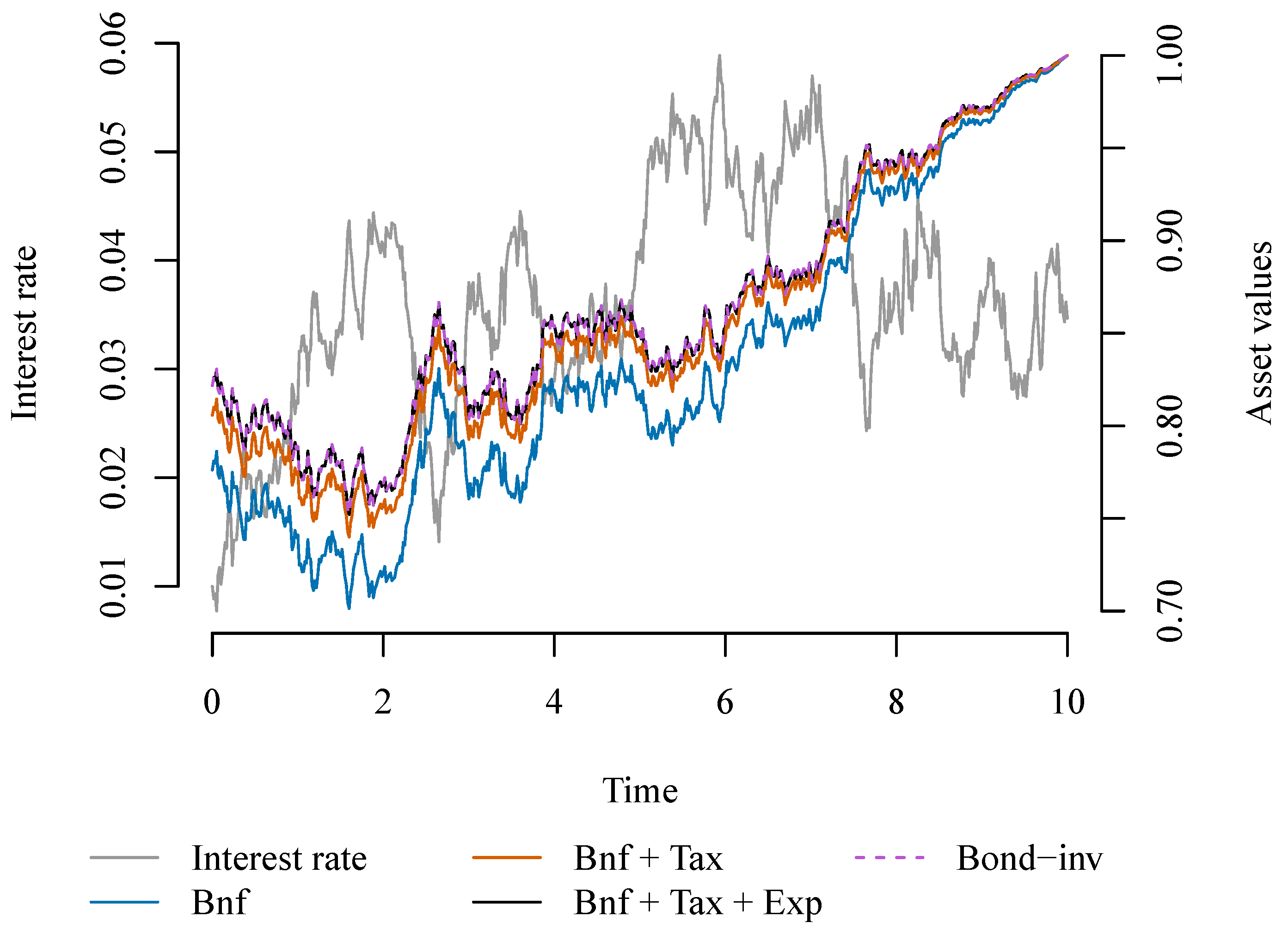
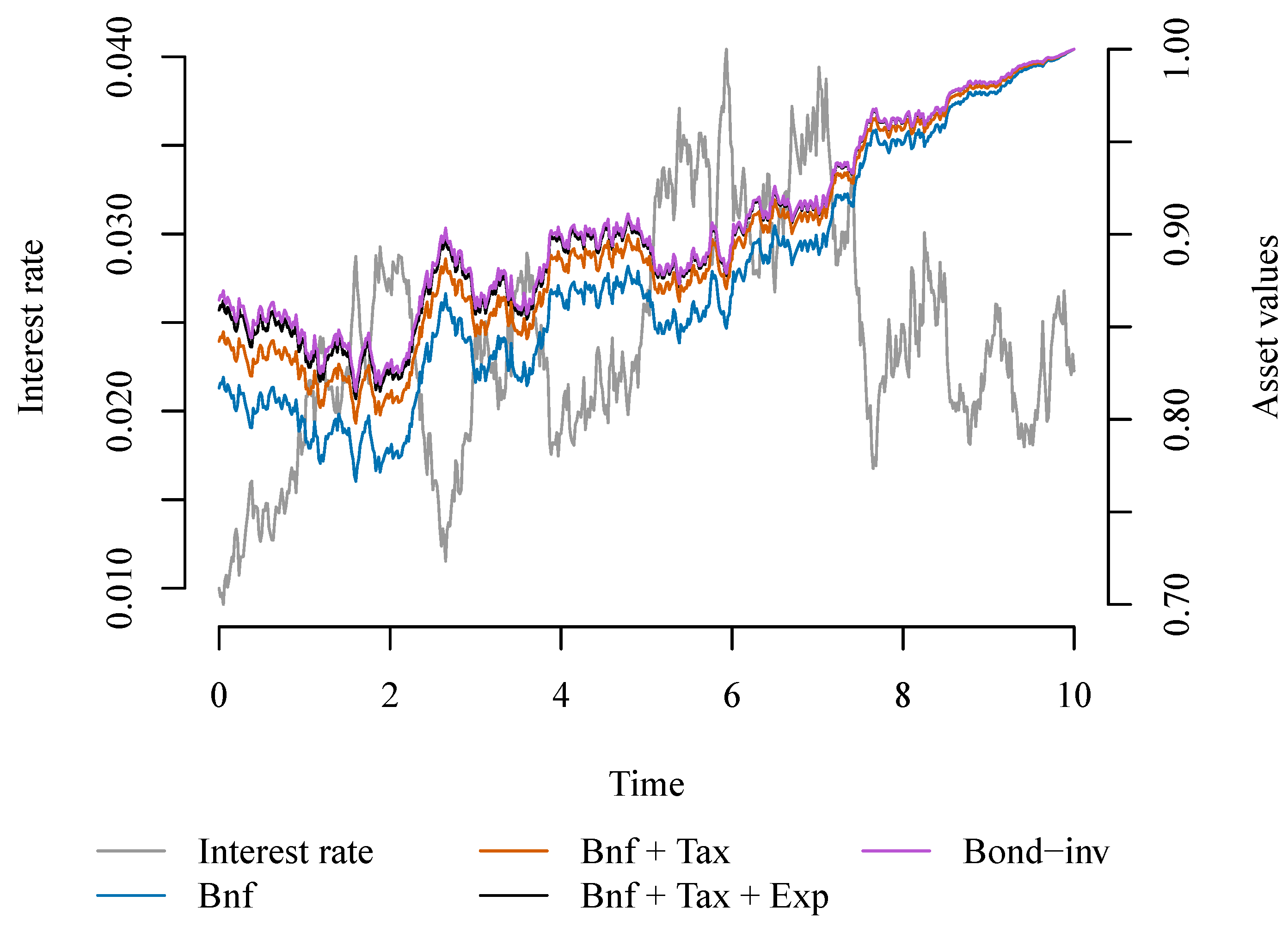
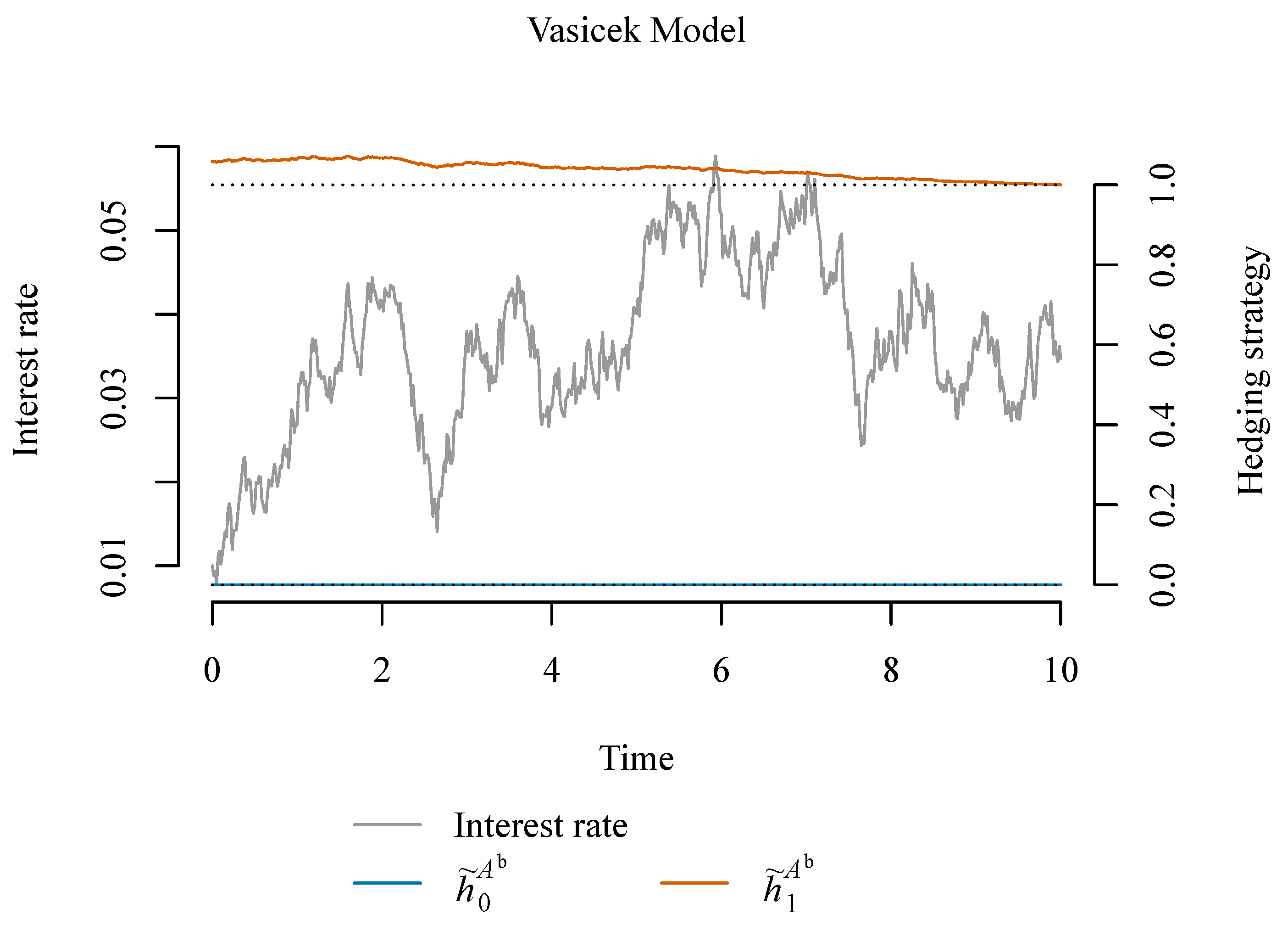
We illustrate the value of the benefit payment, the taxes and the expenses during a single sample path of the market; see Figure 1 for the Vasicek model and Figure 2 for the CIR model. The sample paths in the two figures are based on the same underlying sample path of W. The associated hedging strategies of the total investment ${\tilde{h}}^{A^{\mathrm{b}}}$ are illustrated in Figure 3 for the Vasicek model and Figure 4 for the CIR model.

From the illustrations, we see that in the Vasicek model, the total investment is in the zero coupon bond. We already knew that in order to hedge the benefit payment alone, one must buy a single bond. To additionally hedge the expense and tax payments, the hedging strategy is equally simple, albeit the bonds must be sold continuously during the time period in order to pay the continuously-incurred expenses and tax payments.

In the CIR model, there is a (small) negative investment in the bank account (see Figure 4), such that the investment in the bond is leveraged. The hedging of the expense and tax payments thus leads to a non-trivial investment in the bond and bank account.

5.1. Valuation with Forward Rates

In Section 3.2, we saw an inequality relation to a simple valuation based on the forward rates. The value of the payment at time t is given as (51), and in Section 3.2, we saw that:

$$\begin{array}{cc}V({\tilde{h}}^{A^{\mathrm{b}}},t)\hfill & =E^Q\left[\left.e^{-{\int }_t^T((1-\gamma )r\left(u\right)-\delta )\mathrm{d}u}\right|\mathcal{F}\left(t\right)\right]\hfill \\ & \le e^{-{\int }_t^T((1-\gamma )f(t,u)-\delta )\mathrm{d}u}.\hfill \end{array}$$

Thus, if one has access to a forward interest rate curve, we can obtain an upper bound for the value, which holds for any interest rate model. An interesting question is how big the difference is. The difference scales with the size of the volatility, and if the volatility is zero, corresponding to a deterministic interest rate curve, the forward rate-based approach is correct.

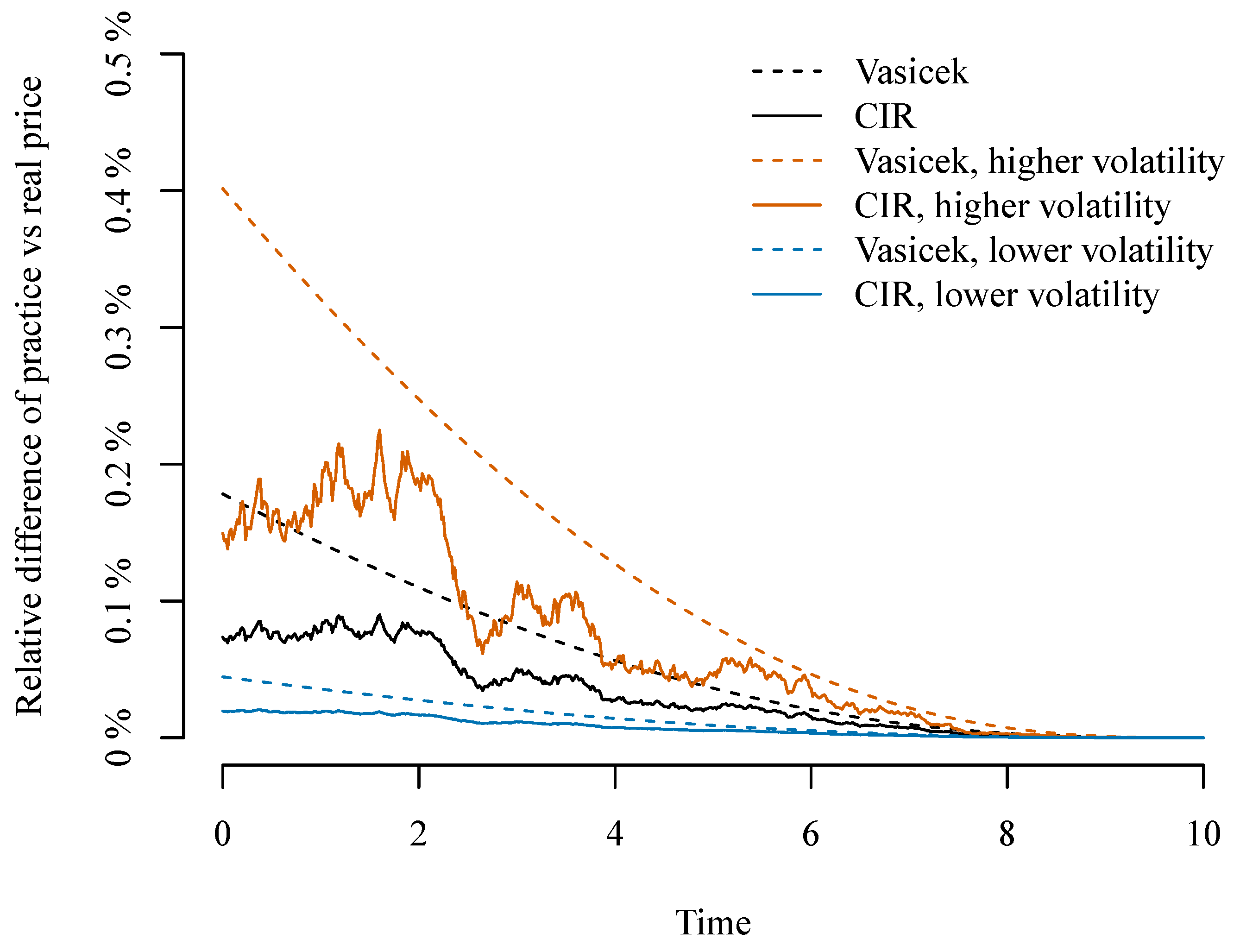
In Figure 5, we illustrate the difference between the theoretical prices in the presence of taxes and expenses and the approximation based on the forward interest rate,

$$\begin{array}{c}t\mapsto \frac{e^{-{\int }_t^T((1-\gamma )f(t,u)-\delta )\mathrm{d}u}}{E^Q\left[\left.e^{-{\int }_t^T((1-\gamma )r\left(u\right)-\delta )\mathrm{d}u}\right|\mathcal{F}\left(t\right)\right]}-1.\hfill \end{array}$$

The illustration is done as a function of time to maturity, using the simulated interest rate path. Different volatilities are illustrated. The difference scales with volatility, and an interesting observation is that the difference is smooth for the Vasicek model only. This can be interpreted as due to the fact that the volatility in the Vasicek model is independent of the interest rate level and that it therefore does not vary with the interest rate simulation. On the other hand, in the CIR model, the volatility scales with the interest rate, and therefore, the difference is dependent on the particular interest rate path.

5.2. A Short Overview of the Main Results in the Numerical Example

In Section 5, we have presented a numerical example, which allows for a comparison of the theoretical valuation formula obtained in Section 3 and the method typically applied in the Danish insurance accounting practice, where the forward rates are modified directly in order to account for the tax rate. We have compared these two methods for the Vasicek model and the CIR model and for various choices of the volatility parameter.

For the Vasicek model, the market values obtained with the method applied in practice are up to 0.2% larger than the theoretical value for reasonable choices of the volatility parameter and the time horizon; for the CIR model, the differences are smaller. With larger values of the volatility, the difference between the two methods increases. The numerical study confirms that the current market practice is conservative and can be viewed as a good approximation for the theoretical values obtained in a setting with continuously-payable expenses and symmetric taxes. Hence, our results can be viewed as a justification for the current market practice method.

References

- Björk, Tomas. 2004. Arbitrage Theory in Continuous Time, 2nd ed.Oxford University Press: Oxford. [Google Scholar]
- Buchardt, Kristian. 2016. Continuous affine processes: Transformations, Markov chains and life insurance. Advances in Applied Probability 48: 423–42. [Google Scholar] [CrossRef]
- Damgaard, Anders. 2003. Utility based option evaluation with proportional transaction costs. Journal of Economic Dynamics and Control 27: 667–700. [Google Scholar] [CrossRef]
- Damgaard, Anders. 2006. Computation of reservation prices for options with proportional transaction costs. Journal of Economic Dynamics and Control 30: 415–44. [Google Scholar] [CrossRef]
- European Insurance and Occupational Pensions Authority (EIOPA). 2009. Solvency II Directive (Directive 2009/138/EC). The European Parliament and the Council of the European Union. Frankfurt: EIOPA. [Google Scholar]
- European Insurance and Occupational Pensions Authority (EIOPA). 2015. Commission Delegated Regulation (EU) 2015/35 of 10 October 2014 Supplementing Directive 2009/138/EC of the European Parliament and of the Council on the Taking-Up and Pursuit of the Business of Insurance and Reinsurance (Solvency II). Frankfurt: EIOPA. [Google Scholar]
- Filipovic, Damir. 2009. Term Structure Models. Spring Finance. Berlin: Springer. [Google Scholar]
- Leland, Hayne E. 1985. Option pricing and replication with transactions costs. The Journal of Finance 40: 1281–301. [Google Scholar] [CrossRef]
- McCulloch, J. Huston. 1975. The tax-adjusted yield curve. The Journal of Finance 30: 811–30. [Google Scholar] [CrossRef]
- Møller, Thomas. 2001. Risk-minimizing hedging strategies for insurance payment processes. Finance and Stochastics 5: 419–46. [Google Scholar] [CrossRef]
- Møller, Thomas, and Mogens Steffensen. 2007. Market-Valuation Methods in Life and Pension Insurance. International Series on Actuarial Science. Cambridge: Cambridge University Press. [Google Scholar]
- Soner, Halil M., Steven E. Shreve, and Jaksa Cvitanic. 1995. There is no nontrivial hedging portfolio for option pricing with transaction costs. Annals of Applied Probability 5: 327–55. [Google Scholar] [CrossRef]
Figure 1.
A simulated path for the Vasicek interest rate model (left axis) and relevant associated value processes (right axis). The total value of the hedging portfolio is illustrated as the black line “Bnf + Tax + Exp”. The value of the benefits alone is illustrated as the blue line “Bnf”, and the value of the benefit and tax payments is illustrated as the red line “Bnf + Tax”. The value of the investment in the bond (the dashed purple line “Bond-inv”) is, here in the Vasicek case, identical to the value of the whole hedging portfolio and therefore coincides with the black line “Bnf + Tax + Exp”.
Figure 2.
A simulated path for the CIR interest rate model (left axis) and relevant associated value processes (right axis). The illustrated lines are similar to Figure 1. Here, in the CIR case, the value of the investment in the bond does not coincide with the total value of the hedging portfolio, and in particular, we see that the value of the bond investment (the purple line “Bond-inv”) is larger than the value of the portfolio, because the investment in the bond is leveraged.
Figure 3.
A simulated path for the Vasicek interest rate model (left axis) and the hedging strategy and in the presence of taxes and expenses (right axis). As we argued above, here in the Vasicek case, the investment in the bank is zero corresponding to . We see that we buy a bit more than one bond, and the difference in value is the value of the tax and expense payments combined.
Figure 4.
A simulated path for the CIR interest rate model (left axis) and the hedging strategy and in the presence of taxes and expenses (right axis). In this (the CIR) case, there is a small investment in the bank account.
Figure 5.
Difference between the approximation based on the forward interest rate curve and the correct theoretical prices in the Vasicek and CIR models. The Vasicek and CIR models with parameters from Table 1 are shown, as well as two variations, where the volatilities are scaled up respectively down by 50%. The approximated value overestimates the correct value by 0.01–0.4% in our numerical examples.