Extreme Portfolio Loss Correlations in Credit Risk

Abstract

The stability of the financial system is associated with systemic risk factors such as the concurrent default of numerous small obligors. Hence, it is of utmost importance to study the mutual dependence of losses for different creditors in the case of large, overlapping credit portfolios. We analytically calculate the multivariate joint loss distribution of several credit portfolios on a non-stationary market. To take fluctuating asset correlations into account, we use an random matrix approach which preserves, as a much appreciated side effect, analytical tractability and drastically reduces the number of parameters. We show that, for two disjoint credit portfolios, diversification does not work in a correlated market. Additionally, we find large concurrent portfolio losses to be rather likely. We show that significant correlations of the losses emerge not only for large portfolios with thousands of credit contracts, but also for small portfolios consisting of a few credit contracts only. Furthermore, we include subordination levels, which were established in collateralized debt obligations to protect the more senior tranches from high losses. We analytically corroborate the observation that an extreme loss of the subordinated creditor is likely to also yield a large loss of the senior creditor.

1. Introduction

The subprime crisis 2007–2009 had a drastic influence on the world economy, due to the almost concurrent default of many small debtors (Hull 2009). Most of the credit contracts where bundled into credit portfolios in the form of collateralized debt obligations (CDOs). Realistic estimates for credit risks and the possible losses, particularly of large portfolios are important not only for the creditors, also and maybe even more from a systemic viewpoint. There is a wealth of studies on credit risk (see (Bielecki and Rutkowski 2013; Bluhm et al. 2016; Chava et al. 2011; Crouhy et al. 2000; Duffie and Singleton 1999; Glasserman and Ruiz-Mata 2006; Heitfield et al. 2006; Lando 2009; Mainik and Embrechts 2013; McNeil et al. 2005; Schönbucher 2003) and references therein). For a review on credit contagion, see (Avkiran et al. 2018; Egloff et al. 2007; Giesecke and Weber 2004 2006; Hatchett and Kühn 2009), and, for studies on practical investment and Value-at-Risk applications of copula theory in evaluating systemic risk, see (Low et al. 2013; Low 2017).

In a credit portfolio, it is of utmost importance to consider the correlations of the asset values. It has been shown that in the presence of even little correlations the concept of diversification is deeply flawed (Glasserman 2004; Schäfer et al. 2007; Schmitt et al. 2014, 2015; Schönbucher 2001). Hence, it is not possible to lower the tail risk significantly by enlarging the number of credit contracts in a credit portfolio. In general, diversification is not always fruitful (Bardoscia et al. 2017; Corsi et al. 2016; Humphrey et al. 2015; Ibragimov and Walden 2007; Wagner 2010).

To obtain a comprehensive understanding of systemic credit risk, it is important to study and model the mutual dependence of losses of different portfolios. Here, we are interested in the joint probability distribution that contains all the information on the individual loss distributions as well as their dependence structure. We apply the Merton (1974) model to several credit portfolios simultaneously (Münnix et al. 2014). Additionally, we take fluctuating asset correlations into account. These emerge because of the intrinsic non-stationarity of financial markets, which leads to a change of the correlation and covariance matrix in time (Münnix et al. 2012; Sandoval and Franca 2012; Schmitt et al. 2013; Song et al. 2011). To describe this non-stationarity, we use an random matrix approach that was recently introduced (Chetalova et al. 2015); for a comprehensive review, see (Mühlbacher and Guhr 2018). It results in a multivariate asset return distribution averaged over the fluctuating correlation matrices. The validity of this approach has been confirmed by empirical data analysis (Schmitt et al. 2013, 2015). The random matrix approach leads to a drastic reduction of the number of parameters describing the distribution. Remarkably, only two parameters, the average correlation coefficient of the asset values and the strength of the fluctuations are sufficient. The standard method for the Merton model does merely incorporate stationary asset correlations, whereas our model takes non-stationary asset correlations into account. This is an important feature that has a significant influence on the tail of the loss distribution. Furthermore, the random matrix approach reduces the numbers of relevant parameters significantly. With only two parameters, we are able to approximate the formidable complexity of the return distribution of a financial market very well.

From the asset return distribution, we analytically derive a joint probability distribution of credit portfolio losses. In addition, we derive a limiting distribution for infinitely large credit portfolios (Lucas et al. 2001). We analyze in detail two non-overlapping credit portfolios that operate on the same market. Moreover, we include subordination levels (An et al. 2015; Black and Cox 1976; Gorton and Santomero 1990). At maturity time, the senior creditor is paid out first and the junior subordinated creditor is only paid out if the senior creditor regained the full promised payment. This is related to CDO tranches and gives further information on to multivariate credit risk (Benmelech and Dlugosz 2009; Duffie and Garleanu 2001; Longstaff and Rajan 2008).

Furthermore, we consider a single credit portfolio that operates on several markets which are on average uncorrelated. We are able to derive a limiting distribution for an infinitely large credit portfolio. Here, the tail risk is lower than in the case of one market with effective average correlation structure, but still diversification is limited.

The paper is organized as follows. In Section 2, we introduce the Merton model and derive the portfolio loss distributions for different debt structures. In Section 3, we present our results for empirical estimated parameters. We conclude our observations in Section 4.

2. Model

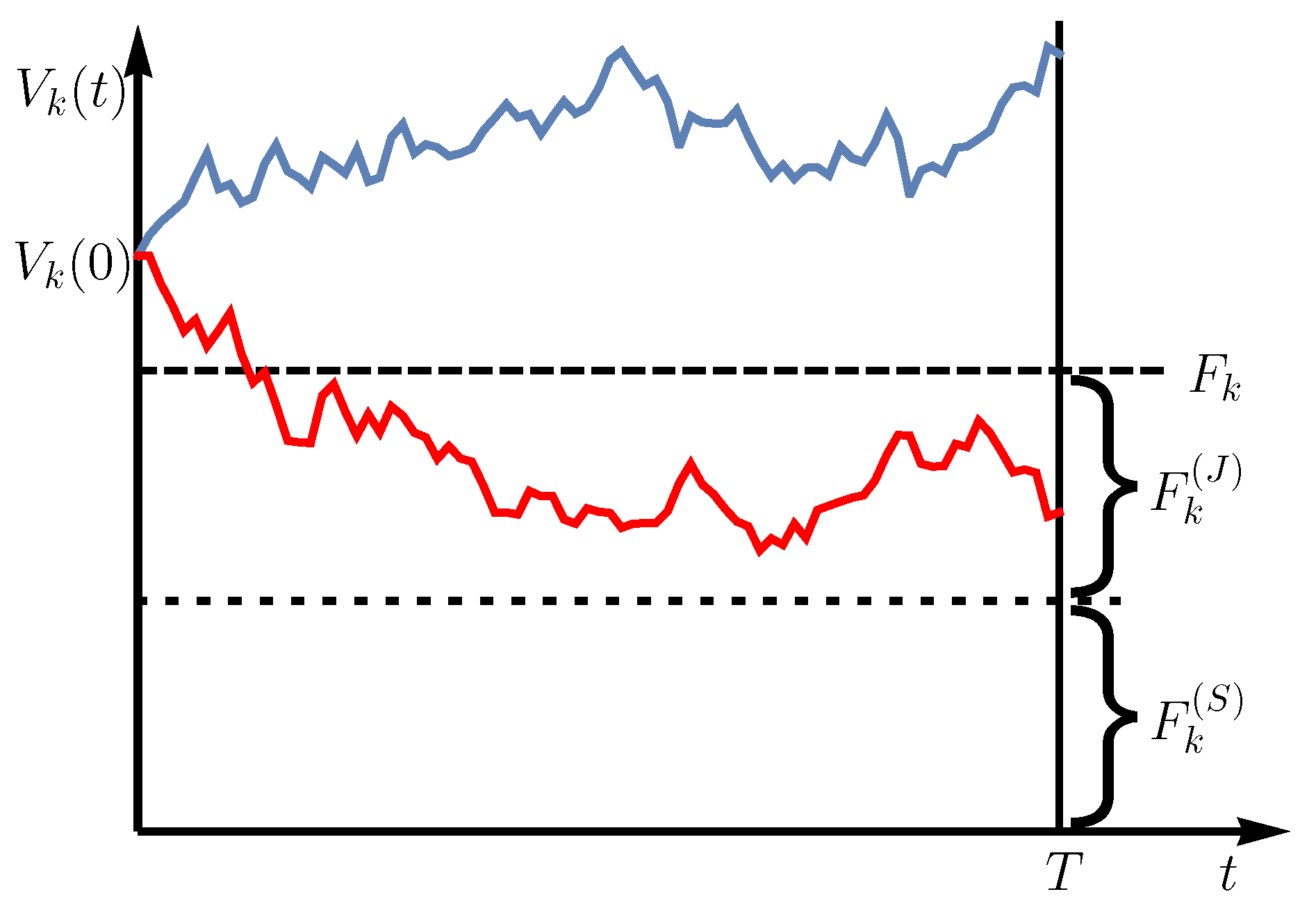
We extend the Merton model to a multivariate scenario with two creditors and K correlated obligors with asset values or economic states $V_k(t)$, $k=1,\dots ,K$ at time t. Each obligor may hold a credit contract from each creditor. In the Merton model, the asset values $V_k(t)$ are estimated by the stock prices of the corresponding obligors. Thus, we assume that all K obligors are companies that can be traded on a stock market. We claim that the asset values follow a geometric Brownian motion. Furthermore, we assume subordinated debt where at maturity time T the senior creditor is paid out first and the junior subordinated creditor is only paid out if the senior creditor regained the full promised payment. Suppose each obligor has to pay back the face value $F_k$ at maturity time T. We consider large time scales such as one year or one month. The face value of each obligor is composed of the face value of the senior creditor $F_k^{(S)}$ and the face value of the junior subordinated creditor $F_k^{(J)}$, which is $F_k=F_k^{(S)}+F_k^{(J)}$. A default occurs if the asset value drops below the face value i.e., $V_k(T)<F_k$ for at least one obligor. The severity of the loss depends on the value of the obligors $V(T)$ at time maturity. For $F_k>V_k(T)>F_k^{(S)}$, the default is completely defrayed by the junior subordinated creditor meaning that the senior creditor does not incur any loss. The senior creditor will incur a loss while the junior subordinated creditor will sustain a total loss only if $V_k(T)<F_k^{(S)}$ t. A visualization of the underlying process for a single asset is shown in Figure 1.

The colored lines show two time-dependent asset values $V_k(t)$. In the blue case, the asset value of the company at maturity is above the face value and the promised payment can be made. In the red case, the asset value at maturity is below the total face value $F_k$ but still above the face value of the senior creditor $F_k^{(S)}$, which results in a default of the junior creditor, while the senior creditor regains the full promised payment.

The normalized loss $L_k^{(S)}$ that a senior creditor and the normalized loss $L_k^{(J)}$ that a junior subordinated creditor is suffering can be expressed as

$$\begin{array}{ccc}\hfill L_k^{(S)}=& \left(1-\frac{V_k(T)}{F_k^{(S)}}\right)\mathsf{\Theta }\left(F_k^{(S)}-V_k(T)\right),\hfill & \hfill (1)\\ \hfill L_k^{(J)}=& \left(1-\frac{V_k(T)-F_k^{(S)}}{F_k^{(J)}}\mathsf{\Theta }\left(V_k(T)-F_k^{(S)}\right)\right)\mathsf{\Theta }\left(F_k-V_k(T)\right),\hfill & \hfill (2)\end{array}$$

respectively. The Heaviside step functions

$$\begin{array}{c}\hfill \mathsf{\Theta }(x)=\left\{\begin{array}{cc}0,\hfill & x<0,\hfill \\ \frac{1}{2},\hfill & x=0,\hfill \\ 1,\hfill & x>0,\hfill \end{array}\right.\end{array}$$

(3)

ensure that the losses are strictly positive. We introduce the fractional face values $f_k^{(S)}$ and $f_k^{(J)}$ for the senior and junior subordinated creditors

$$\begin{array}{c}\hfill f_k^{(S)}=\frac{F_k^{(S)}}{{\sum }_{l=1}^K{F}_l^{(S)}}\mathrm{and}{f}_k^{(J)}=\frac{F_k^{(J)}}{{\sum }_{l=1}^K{F}_l^{(J)}},\end{array}$$

(4)

respectively. This enables us to define the normalized portfolio losses $L^{(S)}$ and $L^{(J)}$ for the senior and junior subordinated creditors as weighted sums

$$\begin{array}{c}\hfill L^{(S)}=\sum _{k=1}^K{f}_k^{(S)}{L}_k^{(S)}\mathrm{and}{L}^{(J)}=\sum _{k=1}^K{f}_k^{(J)}{L}_k^{(J)},\end{array}$$

(5)

respectively. Our aim is to derive the bivariate distribution $p(L^{(S)},L^{(J)}|\mathsf{\Sigma })$ of the portfolio losses, which depends on the covariance matrix $\mathsf{\Sigma }$. This can be done by integrating over all portfolio values and filtering those that lead to a given bivariate total loss $(L^{(S)},L^{(J)})$

$$\begin{array}{c}\hfill p(L^{(S)},L^{(J)}|\mathsf{\Sigma })=\int d\left[V\right]g(V|\mathsf{\Sigma })\delta \left(L^{(S)}-\sum _{k=1}^K{f}_k^{(S)}{L}_k^{(S)}\right)\delta \left(L^{(J)}-\sum _{k=1}^K{f}_k^{(J)}{L}_k^{(J)}\right),\end{array}$$

(6)

where $g(V|\mathsf{\Sigma })$ is the multivariate distribution of the correlated asset values of the obligors at maturity, $\mathsf{\Sigma }$ is the covariance matrix of the asset values, which is in our model well estimated by that of the stock prices. $\delta (x)$ is the Dirac delta function and $V=(V_1(T),\dots ,V_K(T))$ is the K component vector of the asset values. The measure $d\left[V\right]$ is the product of all differentials $d{V}_k$ and the integration domain ranges from zero to infinity for every integral. Using the Fourier representation of the $\delta$ function (Lighthill 1958) as well as Equations (1) and (2), we find

$$\begin{array}{cc}\hfill p(L^{(S)},L^{(J)}|\mathsf{\Sigma })=& \frac{1}{{(2\pi )}^2}\underset{-\infty }{\overset{\infty }{\int }}d{\nu }^{(S)}{e}^{-i{\nu }^{(S)}{L}^{(S)}}\underset{-\infty }{\overset{\infty }{\int }}d{\nu }^{(J)}{e}^{-i{\nu }^{(J)}{L}^{(J)}}\hfill \\ & \times \prod _{k=1}^K\left[\underset{0}{\overset{F_k^{(S)}}{\int }}d{V}_{k}exp\left(i{\nu }^{(S)}{f}_k^{(S)}\left(1-\frac{V_k}{F_k^{(S)}}\right)+i{\nu }^{(J)}{f}_k^{(J)}\right)\right.\hfill \\ & +\left.\underset{F_k^{(S)}}{\overset{F_k}{\int }}d{V}_{k}exp\left(i{\nu }^{(J)}{f}_k^{(J)}\left(1-\frac{V_k-F_k^{(S)}}{F_k^{(J)}}\right)\right)+\underset{F_k}{\overset{\infty }{\int }}d{V}_k\right]g(V|\mathsf{\Sigma }),\hfill \end{array}$$

(7)

where we split the $V_k$ integrals in three parts. We will use this expression later on, but we first need to specify the multivariate distribution of the correlated asset values $g(V|\mathsf{\Sigma })$.

Our goal is to calculate average joint loss distributions that take the non-stationarity of the covariances into account

$$\begin{array}{c}\hfill \langle p\rangle (L^{(S)},L^{(J)}|\mathsf{\Sigma })=\int d\left[V\right]\langle g\rangle (V|\mathsf{\Sigma })\delta \left(L^{(S)}-\sum _{k=1}^K{f}_k^{(S)}{L}_k^{(S)}\right)\delta \left(L^{(J)}-\sum _{k=1}^K{f}_k^{(J)}{L}_k^{(J)}\right)\end{array}$$

(8)

and according to Equation (7). We will argue that this is achieved by properly averaging the multivariate distribution $g(V|\mathsf{\Sigma })$, resulting in $\langle g\rangle (V|\mathsf{\Sigma })$.

2.1. Average Distribution

Following (Schmitt et al. 2013, 2015) and (Münnix et al. 2014), we use a random matrix concept to capture the non-stationarity of the correlations between the asset values $V_k$. The covariances of the returns

$$\begin{array}{c}\hfill r_k(t)=\frac{V_k(t+\mathsf{\Delta }t)-V_k(t)}{V_k(t)},\end{array}$$

(9)

with the return interval $\mathsf{\Delta }t$ are ordered in the $K\times K$ covariance matrix $\mathsf{\Sigma }$. It can be expressed as $\mathsf{\Sigma }=\sigma C\sigma$ with the correlation matrix C and the diagonal matrix $\sigma =diag\left({\sigma }_1,\dots ,{\sigma }_K\right)$ containing the volatilities of the different return time series $r_k$.

In short time intervals where the covariance matrices can be viewed as stationary, the asset return distribution is a multivariate Gaussian $g_s(r|\mathsf{\Sigma })$ (Schmitt et al. 2013). Importantly, we are interested in longer time intervals where non-stationarity is present in the covariances. As the covariance matrices differ significantly for different times, we empirically obtain an existing ensemble of different covariance matrices. These covariance matrices can be modeled by means of $K\times N$ random matrices W, which contain as rows the model time series. Thus, $W{W}^{†}/N$ is the model random covariance matrix and we replace

$$\begin{array}{c}\hfill \mathsf{\Sigma }\to \frac{1}{N}W{W}^{†},\end{array}$$

(10)

where we are free to choose the length N of the model time series. The symbol † denotes the transpose of a vector or matrix. The larger N, the more terms contribute to the elements of the model covariance matrix $W{W}^{†}/N$. In (Münnix et al. 2014; Schmitt et al. 2013, 2015), it was demonstrated that the empirical data ensemble can be very efficiently modeled by such random matrices W distributed according to Wishart (1928)

$$\begin{array}{c}\hfill w(W|{\mathsf{\Sigma }}_0,N)=\frac{{\sqrt{N}}^{KN}}{{\sqrt{det(2\pi {\mathsf{\Sigma }}_0)}}^N}exp\left(-\frac{N}{2}tr{W}^{†}{\mathsf{\Sigma }}_0^{-1}W\right).\end{array}$$

(11)

This distribution defines an ensemble of random covariance matrices $W{W}^{†}/N$ which fluctuate around the average covariance matrix ${\mathsf{\Sigma }}_0$ that is empirically evaluated over the whole time interval. In the limit $N\to \infty$, the Wishart distribution fixes the random matrices $W{W}^{†}/N$ to the average covariance matrix ${\mathsf{\Sigma }}_0$, which is empirical input. Hence, we replace the covariance matrices $\mathsf{\Sigma }$ with the random matrices $W{W}^{†}/N$ according to (10) and average over the Wishart ensemble (11) to account for the non-stationarity. The ensemble average leads to the following general result for the average return distribution in the presence of fluctuating covariance matrices,

$$\begin{array}{c}\hfill 〈g〉\left(r|{\mathsf{\Sigma }}_0,N\right)=\frac{{\sqrt{N}}^K}{{\sqrt{2}}^{N-2}\mathsf{\Gamma }(N/2)\sqrt{det(2\pi {\mathsf{\Sigma }}_0)}}\frac{{\mathcal{K}}_{(K-N)/2}\left(\sqrt{N{r}^{†}{\mathsf{\Sigma }}_0^{-1}r}\right)}{{\sqrt{N{r}^{†}{\mathsf{\Sigma }}_0^{-1}r}}^{(K-N)/2}},\end{array}$$

(12)

where ${\mathcal{K}}_{(K-N)/2}$ is the Bessel function of second kind and of order $(K-N)/2$ (Schmitt et al. 2013). ${\mathsf{\Sigma }}_0$ is the covariance matrix averaged over the whole data interval considered and N controls the strength of the fluctuations around the average covariance matrix ${\mathsf{\Sigma }}_0$. The smaller N, the larger are the fluctuations. In this notation and all further notations, we omit the time dependences of r and V. Hence, the heavier the tails of the distribution (12), the smaller the N. The distribution is very non-Gaussian and differs considerably from $g_s(r|\mathsf{\Sigma })$. Since we assume all credit contracts to have the form of zero coupon bonds, we consider our return intervals to have the same length as the maturity time, i.e., $\mathsf{\Delta }t=T$.

Refs. (Schmitt et al. 2013, 2015) have shown that an effective average correlation matrix of the form

$$\begin{array}{c}\hfill C=(1-c){\mathrm{𝟙}}_K+c{e}_K{e}_K^{†}=\left[\begin{array}{cccc}1& c& c& \dots \\ c& 1& c& \dots \\ c& c& 1& \dots \\ ⋮& ⋮& ⋮& \ddots \end{array}\right],\end{array}$$

(13)

with ${\mathrm{𝟙}}_K$ being the $K\times K$ unit matrix and $e_K$ being a K component vector containing ones, yields a good description of empirical data in the present setting. If we studied non-averaged quantities depending on a specific correlation structure, this approach would be much less likely to give satisfactory results. The choice has two major advantages. First, we achieve analytical tractability, which can be seen later on in Section 2.2; second, we can describe the complexity of a correlated market with only two parameters. The first parameter c is an effective average correlation coefficient and the second parameter N describes the strength of the fluctuations around this average. Both parameters have to be estimated from empirical data.

Due to the fact that we need the asset values $V_k(T)$ in our loss distribution (6) while covariances are measured by means of returns, we have to perform a change of variables using Itô’s lemma (Itô 1944)

$$\begin{array}{c}\hfill r_k\to ln\frac{V_k(T)}{V_{k0}}-\left({\mu }_k-\frac{{\rho }_k^2}{2}\right)T,\end{array}$$

(14)

where $V_{k0}=V_k(0)$ is the initial asset value. This is a geometric Brownian motion with drift ${\mu }_k$ and volatility ${\rho }_k$ with ${\sigma }_k={\rho }_k\sqrt{T}$, where ${\sigma }_k$ is the sample standard deviation. Expression (12) can now be rewritten using Fourier integrals. After employing and adjusting the steps in (Schmitt et al. 2014), we arrive at the double integral

$$\begin{array}{cc}\hfill 〈g〉\left(V|c,N\right)=& \frac{1}{2^{N/2}\mathsf{\Gamma }(N/2)}\underset{0}{\overset{\infty }{\int }}dz{z}^{N/2-1}{e}^{-z/2}\sqrt{\frac{N}{2\pi z}}{\sqrt{\frac{N}{2\pi z(1-c)T}}}^K\underset{-\infty }{\overset{\infty }{\int }}duexp\left(-\frac{N}{2z}{u}^2\right)\hfill \\ & \times \prod _{k=1}^K\frac{1}{V_k{\rho }_k}exp\left[-\frac{N}{2z(1-c)T{\rho }_k^2}{\left(ln\frac{V_k}{V_{k0}}-\left({\mu }_k-\frac{{\rho }_k^2}{2}\right)T+\sqrt{cT}u{\rho }_k\right)}^2\right].\hfill \end{array}$$

(15)

The random matrix model of non-stationarity together with the effective average correlation matrix results in an expression for the joint multivariate distribution of the asset values in terms of a bivariate average of the product of geometric Brownian motions over a ${\chi }^2$ distribution in z and a Gaussian in u. We do not perform the u integration yet because we will factorize the $V_k$ integrals when computing the loss distribution (6) later on.

Several on Average Uncorrelated Markets

To be more realistic, we consider not just one market but several markets that are, on average, uncorrelated. This is an extension of unpublished work by (Nitschke 2014). We define the number of uncorrelated markets to be $\beta$. In this case, the correlation matrix $C=diag(C_1,\dots ,C_{\beta })$ is block diagonal where $C_l=(1-c_l){\mathrm{𝟙}}_{K_l}+c_l{e}_{K_l}{e}_{K_l}^{†}$ are matrices themselves with dimensions $K_l\times K_l$ for $l\in \{1,\dots ,\beta \}$. The correlation matrix C has dimension $K\times K$ and therefore ${\sum }_{l=1}^{\beta }{K}_l=K$ holds. This block structure in not reflected in the random correlation matrices fluctuating about C (see Equation (11)). Hence, there are correlations between the blocks, only their average is zero. The correlation structure allows us to study the impact when going from one market to several markets. Within one market, we again have an on average effectively correlation structure and, across the markets, we have an average correlation of zero. Importantly, this only means the absence of correlations on average. The correlations in our model and in reality fluctuate, implying that in any short instant of time, correlations can be present whose strength is governed by the parameter N. Furthermore, each market has its own standard deviation matrix ${\sigma }_l=diag({\sigma }_{l1},\dots ,{\sigma }_{l{K}_l})$ and drift vector ${\mu }_l={({\mu }_{l1},\dots ,{\mu }_{l{K}_l})}^{†}$ for $l\in \{1,\dots ,\beta \}$. We properly extend the calculations in (Schmitt et al. 2014) with the difference that we have to apply l Fourier integrals, yielding

$$\begin{array}{cc}\hfill 〈g〉\left(V|c,N\right)=& \frac{1}{2^{N/2}\mathsf{\Gamma }(N/2)}\underset{0}{\overset{\infty }{\int }}dz{z}^{N/2-1}{e}^{-z/2}{\sqrt{\frac{N}{2\pi z}}}^{\beta }{\sqrt{\frac{N}{2\pi zT}}}^K\left(\prod _{l=1}^{\beta }\prod _{k=1}^{K_l}\frac{1}{V_{lk}{\rho }_{lk}}\right)\hfill \\ & \times \prod _{l=1}^{\beta }\frac{1}{{\sqrt{1-c_l}}^{K_l}}\underset{-\infty }{\overset{\infty }{\int }}d{u}_{l}exp\left(-\frac{N}{2z}{u}_l^2\right)\hfill \\ & \times exp\left[-\frac{N}{2zT}\sum _k\frac{{\left(ln\frac{V_{lk}}{V_{lk0}}-\left({\mu }_{lk}-\frac{{\rho }_{lk}^2}{2}\right)T+\sqrt{c_{l}T}{u}_l{\rho }_{lk}\right)}^2}{(1-c_l){\rho }_{lk}^2}\right].\hfill \end{array}$$

(16)

This multiple integral depends on the number of markets $\beta$. The index l indicates each market, the index k indicates the asset in a specified market l. In general, the index pair $(l,k)$ denotes the kth asset on the lth market.

2.2. Average Loss Distribution

We work out the average loss distribution (8) using the above results for the average distribution $〈g〉(V|c,N)$. After inserting Equation (15) into Equation (7), we obtain

$$\begin{array}{cc}\hfill 〈p〉(L^{(S)},L^{(J)}|c,N)=& \frac{1}{{(2\pi )}^2{2}^{N/2}\mathsf{\Gamma }(N/2)}\underset{0}{\overset{\infty }{\int }}dz{z}^{N/2-1}{e}^{-z/2}\sqrt{\frac{N}{2\pi z}}\underset{-\infty }{\overset{\infty }{\int }}duexp\left(-\frac{N}{2z}{u}^2\right)\hfill \\ & \times \underset{-\infty }{\overset{\infty }{\int }}d{\nu }^{(S)}{e}^{-i{\nu }^{(S)}{L}^{(S)}}\underset{-\infty }{\overset{\infty }{\int }}d{\nu }^{(J)}{e}^{-i{\nu }^{(J)}{L}^{(J)}}\mathcal{I}\left({\nu }^{(S)},{\nu }^{(J)},z,u\right),\hfill \end{array}$$

(17)

with the term

$$\begin{array}{c}\hfill \mathcal{I}\left({\nu }^{(S)},{\nu }^{(J)},z,u\right)=\prod _{k=1}^K\left\{1+\sum _{j=1}^{\infty }\frac{i^j}{j!}{m}_{j,k}^{(SD)}\left({\nu }^{(S)},{\nu }^{(J)},z,u\right)+\sum _{j=1}^{\infty }\frac{{\left(i{\nu }^{(J)}{f}_k^{(J)}\right)}^j}{j!}{m}_{j,k}^{(J)}\left(z,u\right)\right\}\end{array}$$

(18)

and

$$\begin{array}{c}\hfill m_{a,k}^{(SD)}\left({\nu }^{(S)},{\nu }^{(J)},z,u\right)=\sum _{j=0}^a\left(\genfrac{}{}{0pt}{}{a}{j}\right){\left({\nu }^{(S)}{f}_k^{(S)}\right)}^j{\left({\nu }^{(J)}{f}_k^{(J)}\right)}^{a-j}{m}_{j,k}^{(S)}(z,u)\end{array}$$

(19)

and the moments

$$\begin{array}{cc}\hfill m_{j,k}^{(S)}(z,u)=& \underset{-\infty }{\overset{{\widehat{F}}_k^{(S)}}{\int }}d{\widehat{V}}_k{\left(1-\frac{V_{k0}}{F_k^{(S)}}exp\left(\sqrt{z}{\widehat{V}}_k+\left({\mu }_k-\frac{{\rho }_k^2}{2}\right)T\right)\right)}^j\hfill \\ & \times \sqrt{\frac{N}{2\pi (1-c)T{\rho }_k^2}}exp\left[\frac{N}{2(1-c)T{\rho }_k^2}{\left({\widehat{V}}_k+\sqrt{cT}u{\rho }_k\right)}^2\right]\hfill \end{array}$$

(20)

$$\begin{array}{cc}\hfill m_{j,k}^{(J)}(z,u)& =\underset{{\widehat{F}}_k^{(S)}}{\overset{{\widehat{F}}_k}{\int }}d{\widehat{V}}_k{\left(1+\frac{F_k^{(S)}}{F_k^{(J)}}-\frac{V_{k0}}{F_k^{(J)}}exp\left(\sqrt{z}{\widehat{V}}_k+\left({\mu }_k-\frac{{\rho }_k^2}{2}\right)T\right)\right)}^j\hfill \\ & \times \sqrt{\frac{N}{2\pi (1-c)T{\rho }_k^2}}exp\left[\frac{N}{2(1-c)T{\rho }_k^2}{\left({\widehat{V}}_k+\sqrt{cT}u{\rho }_k\right)}^2\right],\hfill \end{array}$$

(21)

where we use the change of variables ${\widehat{V}}_k=(ln{V}_k/V_{k0}-({\mu }_k-{\rho }_k^2/2)T)/\sqrt{z}$ with proper adjustment of the integration bounds ${\widehat{F}}_k$ and ${\widehat{F}}_k^{(S)}$. The moments $m_{j,k}^{(S)}(z,u)$ and $m_{j,k}^{(J)}(z,u)$ are given in Appendix A for $j=0,1,2$. The term $m_{j,k}^{(SD)}\left({\nu }^{(S)},{\nu }^{(J)},z,u\right)$ formally corresponds to those events that lead to a loss large enough that the senior creditor is affected. We use a binomial sum for the decoupling of the ${\nu }^{(S)}$ and ${\nu }^{(J)}$ integrals later on.

Now, we assume large portfolios where all face values are of the same order, to carry out an approximation to the second order in $f_k^{(S)}$ and $f_k^{(J)}$ by performing steps generalizing the one in (Schmitt et al. 2014). This is justified when we consider all face values are of the same order, so all fractional face values are of order $1/K$. We finally arrive at

$$\begin{array}{cc}\hfill 〈p〉(L^{(S)},L^{(J)}|c,N)=& \frac{1}{2^{N/2}\mathsf{\Gamma }(N/2)}\underset{0}{\overset{\infty }{\int }}dz{z}^{N/2-1}{e}^{-z/2}\sqrt{\frac{N}{2\pi }}\underset{-\infty }{\overset{\infty }{\int }}duexp\left(-\frac{N}{2}{u}^2\right)\hfill \\ & \times \frac{1}{\sqrt{2\pi M_2^{(S)}(z,u)}}exp\left(-\frac{{\left(L^{(S)}-M_1^{(S)}(z,u)\right)}^2}{2M_2^{(S)}(z,u)}\right)\hfill \\ & \times \frac{1}{\sqrt{2\pi M_2(z,u)}}exp\left(-\frac{{\left(L^{(J)}-M_1(L^{(S)},z,u)\right)}^2}{2M_2(z,u)}\right)\hfill \end{array}$$

(22)

for the average distribution with

$$\begin{array}{ccc}\hfill M_1(L^{(S)},z,u)& =M_1^{(J)}(z,u)+\sum _{k=1}^K{f}_k^{(J)}{f}_k^{(S)}{N}_k^{(S)}(z,u)\frac{L^{(S)}-M_1^{(S)}(z,u)}{M_2^{(S)}(z,u)},\hfill & \hfill (23)\\ \hfill M_2(z,u)& =M_2^{(J)}(z,u)-\frac{1}{M_2^{(S)}(z,u)}{\left(\sum _{k=1}^K{f}_k^{(J)}{f}_k^{(S)}{N}_k^{(S)}(z,u)\right)}^2,\hfill & \hfill (24)\\ \hfill M_1^{(S)}(z,u)& =\sum _{k=1}^K{f}_k^{(S)}{m}_{1,k}^{(S)},\hfill & \hfill (25)\\ \hfill M_2^{(S)}(z,u)& =\sum _{k=1}^K{f_k^{(S)}}^2\left(m_{2,k}^{(S)}-{m_{1,k}^{(S)}}^2\right),\hfill & \hfill (26)\\ \hfill M_1^{(J)}(z,u)& =\sum _{k=1}^K{f}_k^{(J)}\left(m_{0,k}^{(S)}+m_{1,k}^{(J)}\right),\hfill & \hfill (27)\\ \hfill M_2^{(J)}(z,u)& =\sum _{k=1}^K{f_k^{(J)}}^2\left(m_{0,k}^{(S)}+m_{2,k}^{(J)}-{m_{0,k}^{(S)}}^2-{m_{1,k}^{(J)}}^2-2m_{0,k}^{(S)}{m}_{1,k}^{(J)}\right),\hfill & \hfill (28)\\ \hfill N_k^{(S)}(z,u)& =m_{1,k}^{(S)}\left(1-m_{0,k}^{(S)}-m_{1,k}^{(J)}\right).\hfill & \hfill (29)\end{array}$$

Thus, we expressed the average loss distribution as double average of Gaussians with mean values $M_1(L^{(S)},z,u)$ and $M_1^{(S)}(z,u)$ and variances $M_2(z,u)$ and $M_2^{(S)}(z,u)$ that non-trivially depend on the integration variables. To keep the notation transparent, we dropped the arguments of the functions $m_{j,k}^{(S)}(z,u)$ and $m_{j,k}^{(J)}(z,u)$. Due to the complexity of the last two expressions in Equation (22), the z and u integrals have to be evaluated numerically. We notice that the normalization of the average distribution is, for $L_k^{(S)},L_k^{(J)}\in [0,1],$ only valid up to the order of our approximation. Later on, we will concentrate on the contributions of no default.

2.3. Homogeneous Portfolio

Apart from the large K approximation, all results above are valid in general and apply to all portfolios for which the individual fractional face values are of order $1/K$. To further evaluate our results and to obtain a visualization, it is instructive to consider homogeneous portfolios, in which the senior and junior face values are equal:

$$\begin{array}{c}\hfill F_k^{(S)}=F_0^{(S)}\mathrm{and}{F}_k^{(J)}=F_0^{(J)},\end{array}$$

(30)

such that

$$\begin{array}{c}\hfill f_k^{(S)}=f_k^{(J)}=\frac{1}{K}.\end{array}$$

(31)

Furthermore, we assume that the stochastic processes have the same initial values, drifts and volatilities,

$$\begin{array}{c}\hfill V_{k0}=V_0,{\mu }_k={\mu }_0,{\rho }_k={\rho }_0.\end{array}$$

(32)

Of course, this does not mean that the realized stochastic processes are the same. By dropping the dependence of k, the moments $m_{a,k}^{(S)}(z,u)=m_{a,0}^{(S)}(z,u)$ and $m_{j,k}^{(J)}(z,u)=m_{j,0}^{(J)}(z,u)$ and thus the average distribution $〈p〉(L^{(S)},L^{(J)})$ can be computed much faster.

2.4. Distribution of the Loss Given Default

Only the full dynamics of our model without any approximations give us information on the contribution of the non-analytic part of the average loss distribution. In particular, absence of losses is reflected in non-analytic $\delta$ functions at zero. To examine this, we start from the averaged version of Equation (7) by inserting the distribution of asset values for a homogeneous portfolio with an effective average correlation matrix

$$\begin{array}{cc}\hfill {〈g〉}_{\mathrm{h}}\left(V|c,N\right)& =\frac{1}{2^{N/2}\mathsf{\Gamma }(N/2)}\underset{0}{\overset{\infty }{\int }}dz{z}^{N/2-1}{e}^{-z/2}\sqrt{\frac{N}{2\pi z}}\underset{-\infty }{\overset{\infty }{\int }}duexp\left(-\frac{N}{2z}{u}^2\right)\hfill \\ & \times {\left(\sqrt{\frac{N}{2\pi z(1-c)T}}\frac{1}{V{\rho }_0}exp\left[-\frac{N}{2z(1-c)T{\rho }_0^2}{\left(ln\frac{V}{V_0}-\left({\mu }_0-\frac{{\rho }_0^2}{2}\right)T+\sqrt{cT}u{\rho }_0\right)}^2\right]\right)}^K\hfill \\ & =\underset{0}{\overset{\infty }{\int }}dz\underset{-\infty }{\overset{\infty }{\int }}duf(z,u){\tilde{\omega }}^K(V,z,u),\hfill \end{array}$$

(33)

with

$$\begin{array}{ccc}\hfill f(z,u)& =\frac{1}{2^{N/2}\mathsf{\Gamma }(N/2)}{z}^{N/2-1}{e}^{-z/2}\sqrt{\frac{N}{2\pi z}}exp\left(-\frac{N}{2z}{u}^2\right)\hfill & \hfill (34)\\ \hfill \tilde{\omega }(V,z,u)& =\sqrt{\frac{N}{2\pi z(1-c)T}}\frac{1}{V{\rho }_0}exp\left[-\frac{N}{2z(1-c)T{\rho }_0^2}{\left(ln\frac{V}{V_0}-\left({\mu }_0-\frac{{\rho }_0^2}{2}\right)T+\sqrt{cT}u{\rho }_0\right)}^2\right].\hfill & \hfill (35)\end{array}$$

Due to the homogeneity, the product in Equation (7) also becomes a K-th power, to which we apply the multinomial theorem. We thus arrive at

$$\begin{array}{cc}\hfill 〈p〉(L^{(S)},L^{(J)}|c,N)=& \underset{0}{\overset{\infty }{\int }}dz\underset{-\infty }{\overset{\infty }{\int }}duf(z,u)\frac{1}{{(2\pi )}^2}\underset{-\infty }{\overset{\infty }{\int }}d{\nu }^{(S)}{e}^{-i{\nu }^{(S)}{L}^{(S)}}\underset{-\infty }{\overset{\infty }{\int }}d{\nu }^{(J)}{e}^{-i{\nu }^{(J)}{L}^{(J)}}\hfill \\ & \times \sum _{k_1+k_2+k_3=K}\left(\genfrac{}{}{0pt}{}{K}{k_1,k_2,k_3}\right){\left(e^{i{\nu }^{(J)}/K}\underset{0}{\overset{F_0^{(S)}}{\int }}dVexp\left(\frac{i{\nu }^{(S)}}{K}\left(1-\frac{V}{F_0^{(S)}}\right)\right)\tilde{\omega }(V,z,u)\right)}^{k_1}\hfill \\ & \times {\left(\underset{F_0^{(S)}}{\overset{F_0}{\int }}dVexp\left(\frac{i{\nu }^{(J)}}{K}\left(1-\frac{V-F_0^{(S)}}{F_0^{(J)}}\right)\right)\tilde{\omega }(V,z,u)\right)}^{k_2}{\left(\underset{F_0}{\overset{\infty }{\int }}dV\tilde{\omega }(V,z,u)\right)}^{k_3}\hfill \end{array}$$

(36)

with the multinomial coefficient

$$\begin{array}{c}\hfill \left(\genfrac{}{}{0pt}{}{K}{k_1,k_2,k_3}\right)=\frac{K!}{k_1!k_2!k_3!}.\end{array}$$

(37)

From Equation (36), we see that $\delta$ functions only appear under the condition $k_1·k_2=0$. For $k_1=k_2=0$, we have no default at all. The only contribution to the distribution stems from the last integral in Equation (36), leading to a $\delta$ peak $\delta (L_k^{(S)})\delta (L_k^{(J)})$ at the origin. This $\delta$ peak is associated with the absence of default neither on the junior nor on the senior level. The probability therefore is

$$\begin{array}{cc}\hfill P^{(\mathrm{ND})}=& \frac{1}{2^{N/2}\mathsf{\Gamma }(N/2)}\underset{0}{\overset{\infty }{\int }}dz{z}^{N/2-1}{e}^{-z/2}\sqrt{\frac{N}{2\pi z}}\underset{-\infty }{\overset{\infty }{\int }}duexp\left(-\frac{N}{2z}{u}^2\right)\hfill \\ & \times {\left(\frac{1}{2}-\frac{1}{2}erf\left[\sqrt{\frac{N}{2z(1-c)T{\rho }_0^2}}\left(ln\frac{F_0}{V_0}-\left({\mu }_0-\frac{{\rho }_0^2}{2}\right)T+\sqrt{cT}u{\rho }_0\right)\right]\right)}^K,\hfill \end{array}$$

(38)

which obviously decreases with increasing K.

For $k_1=0,k_2\ne 0$, we find the contribution of the events that lead to a total junior default but not to a senior default. In this case, we have a single $\delta$ function $\delta (L_k^{(S)})$ that represents a moderate loss such that the senior subordinated creditor will not sustain a loss. The special case $k_1\ne 0,k_2=0$ leads to a sum of $\delta$ functions $\delta (L_k^{(J)}-k_1/K)$ where $k_1$ runs from 1 to K. This is due to the sum in Equation (36). These $\delta$ functions belong to the events where there is either no default at all or $k_1$ severe defaults such that, for $k_1=1,\dots ,K$ obligors, the junior subordinated creditor has a complete failure i.e., $L_k^{(J)}=1$ and the senior subordinated creditor may sustain a loss i.e., $L_k^{(S)}\ge 0$. All of these $\delta$ functions are not unmated but weighted with some integral prefactors to preserve the normalization of the distribution $〈p〉(L^{(S)},L^{(J)})$. Furthermore, the $\delta$ functions disappear when we only consider the loss given default, which in our model means $L^{(J)}>0$ and also $L^{(S)}>0$. The non-analytic parts cannot be obtained in the second order approximation we used to derive the average loss distribution (22).

2.5. Infinitely Large Portfolios

We now consider the case $K\to \infty$ for the homogeneous portfolio to analyze whether diversification works or not in the discussed multivariate scenarios. It has been shown that diversification does not work in a correlated univariate model with only one bank (see (Schmitt et al. 2014)).

The homogeneous versions of Equations (24) and (26)

$$\begin{array}{ccc}\hfill M_2(z,u)& ={\displaystyle \frac{1}{K}}\left(m_{0,0}^{(S)}+m_{2,0}^{(J)}-{m_{0,0}^{(S)}}^2-{m_{1,0}^{(J)}}^2-2m_{0,0}^{(S)}{m}_{1,0}^{(J)}-\frac{{m_{1,0}^{(S)}}^2{\left(1-m_{0,0}^{(S)}-m_{1,0}^{(J)}\right)}^2}{m_{2,0}^{(S)}-{m_{1,0}^{(S)}}^2}\right),\hfill & \hfill (39)\\ \hfill M_2^{(S)}(z,u)& ={\displaystyle \frac{1}{K}}\left(m_{2,0}^{(S)}-{m_{1,0}^{(S)}}^2\right),\hfill & \hfill (40)\end{array}$$

imply that $M_2(z,u)\to 0$ as well as $M_2^{(S)}(z,u)\to 0$ for $K\to \infty$. This means that both Gaussians

$$\begin{array}{c}\hfill \frac{1}{\sqrt{2\pi M_2^{(S)}(z,u)}}exp\left(-\frac{{\left(L^{(S)}-M_1^{(S)}(z,u)\right)}^2}{M_2^{(S)}(z,u)}\right)\mathrm{and}\frac{1}{\sqrt{2\pi M_2(z,u)}}exp\left(-\frac{{\left(L^{(J)}-M_1(L^{(S)},z,u)\right)}^2}{M_2(z,u)}\right)\end{array}$$

in Equation (22) become $\delta$ functions. Thus, we arrive at

$$\begin{array}{ccc}\hfill 〈p〉(L^{(S)},L^{(J)}|c,N){|}_{K\to \infty }& =& \frac{1}{2^{N/2}\mathsf{\Gamma }(N/2)}\underset{0}{\overset{\infty }{\int }}dz{z}^{N/2-1}{e}^{-z/2}\sqrt{\frac{N}{2\pi }}\underset{-\infty }{\overset{\infty }{\int }}duexp\left(-\frac{N}{2}{u}^2\right)\hfill \\ & & \times \delta \left(L^{(S)}-M_1^{(S)}(z,u)\right)\delta \left(L^{(J)}-M_1(L^{(S)},z,u)\right)\hfill \\ & =& \frac{1}{2^{N/2}\mathsf{\Gamma }(N/2)}\underset{0}{\overset{\infty }{\int }}dz{z}^{N/2-1}{e}^{-z/2}\sqrt{\frac{N}{2\pi }}\underset{-\infty }{\overset{\infty }{\int }}duexp\left(-\frac{N}{2}{u}^2\right)\hfill \\ & & \times \delta \left(L^{(S)}-m_{1,0}^{(S)}\right)\delta \left(L^{(J)}-m_{0,0}^{(S)}-m_{1,0}^{(J)}\right).\hfill \end{array}$$

(41)

To make this equation numerically manageable, we use the identity

$$\begin{array}{c}\hfill \delta \left(f(u)\right)=\sum _i\frac{\delta (u-u_i)}{|f^{\prime }(u_i)|},\end{array}$$

(42)

where $u_i$ are the roots of the function $f(u)$, with $f^{\prime }(u_i)\ne 0$. This result is a direct consequence of the elementary theory of distributions (Lighthill 1958). Using this identity three times allows us to solve the remaining two integrals and we finally obtain the limiting loss distribution

$$\begin{array}{cc}\hfill 〈p〉(L^{(S)},L^{(J)}|c,N){|}_{K\to \infty }=& \frac{1}{2^{N/2}\mathsf{\Gamma }(N/2)}\sqrt{\frac{N}{2\pi }}{z}_0^{N/2-1}exp\left(-\frac{z_0}{2}\right)exp\left(-\frac{N}{2}{u^{(S)}}^2(L^{(S)},z_0)\right)\hfill \\ & \times \frac{1}{\left|\frac{\partial }{\partial u}{\left.m_{1,0}^{(S)}(z_0,u)\right|}_{u=u^{(S)}(L^{(S)},z_0)}\right|·\left|\frac{\partial }{\partial u}{\left[m_{0,0}^{(S)}(z_0,u)+m_{1,0}^{(J)}(z_0,u)\right]}_{u=u^{(S)}(L^{(S)},z_0)}\right|}\hfill \\ & \times \frac{1}{\left|\frac{\partial }{\partial z}{\left[u^{(S)}(L^{(S)},z)-u^{(J)}(L^{(J)},z)\right]}_{z=z_0}\right|}.\hfill \end{array}$$

(43)

Here, the implicit functions

$$\begin{array}{ccccc}\hfill u^{(S)}& =u^{(S)}(L^{(S)},z)\hfill & \hfill \mathrm{with}& 0=L^{(S)}-m_{1,0}^{(S)}(z,u^{(S)}),\hfill & \hfill (44)\\ \hfill u^{(J)}& =u^{(J)}(L^{(J)},z)\hfill & \hfill \mathrm{with}& 0=L^{(J)}-m_{0,0}^{(S)}(z,u^{(J)})-m_{1,0}^{(J)}(z,u^{(J)}),\hfill & \hfill (45)\\ \hfill z_0& =z_0(L^{(S)},L^{(J)})\hfill & \hfill \mathrm{with}& u^{(S)}(L^{(S)},z_0)=u^{(J)}(L^{(J)},z_0),\hfill & \hfill (46)\end{array}$$

are unique and have to be calculated numerically. The dependence on $L^{(S)}$ and $L^{(J)}$ is now implicit in the functions $u^{(S)},u^{(J)}$ and $z_0$. The very last derivatives in Equation (43) can be done by using the implicit function theorem. They can be traced back to derivatives of $m_{0,0}^{(S)},m_{1,0}^{(S)}$ and $m_{1,0}^{(J)}$. The functions $m_{1,0}^{(S)}$ and $m_{0,0}^{(S)}+m_{1,0}^{(J)}$ are strictly monotonically increasing in u and z for fixed z and u, respectively. Thus, we can solve Equations (44) and (45) locally to u, where we obtain $u^{(S)}$ and $u^{(J)}$. These equations can be derived by z using

$$\begin{array}{c}\frac{\partial u^{(S)}}{\partial z}(L^{(S)},z_0)=-{\left.\frac{\frac{\partial }{\partial z}{m}_{1,0}^{(S)}(z,u)}{\frac{\partial }{\partial u}{m}_{1,0}^{(S)}(z,u)}\right|}_{u=u^{(S)}(L^{(S)},z_0)}\hfill \end{array}$$

(47)

and

$$\begin{array}{c}\frac{\partial u^{(J)}}{\partial z}(L^{(J)},z_0)=-{\left.\frac{\frac{\partial }{\partial z}\left(m_{0,0}^{(S)}(z,u)+m_{1,0}^{(J)}(z,u)\right)}{\frac{\partial }{\partial u}\left(m_{0,0}^{(S)}(z,u)+m_{1,0}^{(J)}(z,u)\right)}\right|}_{u=u^{(J)}(L^{(J)},z_0)}.\hfill \end{array}$$

(48)

2.6. Absence of Subordination

Now, we consider the same model as discussed before, but without taking subordination into account. This means that a loss is evenly distributed among the creditors. This model is closely related to that in (Sicking et al. 2018). Here, we have $B\ge 2$ creditors with the face value $F_k^{(b)},b=1,\dots ,B,$ $k=1,\dots ,K$ of obligor k within creditor b and the normalized loss according to obligor k

$$\begin{array}{c}\hfill L_k^{(b)}=\left\{\begin{array}{cc}\left(1-\frac{V_k(T)}{F_k}\right)\mathsf{\Theta }\left(F_k-V_k(T)\right)\hfill & \mathrm{if}{F}_k^{(b)}>0,\hfill \\ 0\hfill & \mathrm{else},\hfill \end{array}\right.\end{array}$$

(49)

with the total face value $F_k={\sum }_{b=1}^B{F}_k^{(b)}$ of obligor k and asset value $V_k(t)$. In Equation (49) for $F_k^{(b)}>0$, the losses do not have any dependence on the obligors. In case of default, the creditors are not distinguished and suffer the same normalized loss. Hence, we write $L_k$ instead of $L_k^{(b)}$. Again, we define the normalized portfolio losses $L^{(b)}$ and the fractional face values $f_k^{(b)}$,

$$\begin{array}{c}\hfill L^{(b)}=\sum _{k=1}^K{f}_k^{(b)}{L}_k\mathrm{and}{f}_k^{(b)}=\frac{F_k^{(b)}}{{\displaystyle \sum _{k=1}^K}{F}_k^{(b)}},\end{array}$$

(50)

corresponding to creditor b, respectively. The multivariate distribution of the total average loss is

$$\begin{array}{c}\hfill 〈p〉(L|\mathsf{\Sigma })=\int d\left[V\right]〈g〉(V|\mathsf{\Sigma })\delta \left(L-\sum _{k=1}^K{f}_k{L}_k\right),\end{array}$$

(51)

with $L={(L^{(1)},\dots ,L^{(B)})}^{†}$ and $f_k={(f_k^{(1)},\dots ,f_k^{(B)})}^{†}$. Adjusting our calculations in the subordinated case above and also applying a second order approximation for $f_k^{(b)}$, we arrive at the final result

$$\begin{array}{cc}\hfill 〈p〉(L|c,N)=& \frac{1}{2^{N/2}\mathsf{\Gamma }(N/2)}\underset{0}{\overset{\infty }{\int }}dz{z}^{N/2-1}{e}^{-z/2}\sqrt{\frac{N}{2\pi }}\underset{-\infty }{\overset{\infty }{\int }}duexp\left(-\frac{N}{2}{u}^2\right)\hfill \\ & \times \frac{1}{\sqrt{det\left(2\pi M_2(z,u)\right)}}exp\left(-\frac{1}{2}{\left(L-M_1(z,u)\right)}^{†}{M}_2^{-1}(z,u)\left(L-M_1(z,u)\right)\right),\hfill \end{array}$$

(52)

where

$$\begin{array}{ccc}\hfill M_1(z,u)& =\sum _{k=1}^K{f}_k{m}_{1,k}(z,u),\hfill & \hfill (53)\\ \hfill M_2(z,u)& =\sum _{k=1}^K{D}_k\left(m_{2,k}(z,u)-m_{1,k}^2(z,u)\right),\hfill & \hfill (54)\end{array}$$

with the dyadic matrices

$$\begin{array}{c}\hfill D_k=f_k{f}_k^{†}\end{array}$$

(55)

and with

$$\begin{array}{cc}\hfill m_{j,k}(z,u)=& \underset{-\infty }{\overset{{\widehat{F}}_k}{\int }}d{\widehat{V}}_k{\left(1-\frac{V_{k0}}{F_k}exp\left(\sqrt{z}{\widehat{V}}_k+\left({\mu }_k-\frac{{\rho }_k^2}{2}\right)T\right)\right)}^j\hfill \\ & \times \sqrt{\frac{N}{2\pi (1-c)T{\rho }_k^2}}exp\left[\frac{N}{2(1-c)T{\rho }_k^2}{\left({\widehat{V}}_k+\sqrt{cT}u{\rho }_k\right)}^2\right],\hfill \end{array}$$

(56)

$$\begin{array}{cc}\hfill {\widehat{F}}_k& =\frac{1}{\sqrt{z}}\left(ln\frac{F_k}{V_{k0}}-\left({\mu }_k-\frac{{\rho }_k^2}{2}\right)T\right).\hfill \end{array}$$

(57)

The moments $m_{j,k}(z,u)$ are the same as in Equation (20). For this model, we only consider heterogeneous portfolios for the whole market as homogeneous portfolios would lead to singular matrices $D_k$ as defined in Equation (55), and the losses would be exactly the same for all creditors. Instead, we consider cases where the volume of credit differs among the creditors or we consider cases where the portfolios are non-overlapping or may only partially overlap.

Although our results are general, we now only consider $B=2$ creditors to feasibly render a visualization. We denote them as creditor one and creditor two, respectively. Moreover, we address the most general set-up where two credit portfolios may partially overlap. Again, we consider K obligors in total. Let $R_1$ be the number of obligors with only one credit contract, say from creditor one. Let $R_{12}$ be the number of creditors that raise credits from both creditors. The proportions correspond to the fractions $r_1=R_1/K$ and $r_{12}=R_{12}/K$. Creditor one deals in $R_1+R_{12}$ credits and creditor two deals in $K-R_1$ credits. This model, for example, also includes two disjoint portfolios, and we just have to set $r_{12}=0$. The face value of the $R_{12}$ obligors consist of the sum of two face values $F_k=F_k^{(1)}+F_k^{(2)}$ that do not necessarily have the same size. For later convenience, we consider homogeneous portfolios $F_k=F_0$ and we assume that the face values in the overlapping part of the portfolios are equal within a portfolio but can differ across the portfolios. That means we introduce a parameter $\gamma \in [0,1]$ with $F_k^{(1)}=\gamma F_0$ and $F_k^{(2)}=(1-\gamma )F_0$.

For a market with homogeneous parameters, we find the result (52) with

$$\begin{array}{ccc}\hfill M_1(z,u)& =m_{1,0}(z,u)\left[\begin{array}{c}1\\ 1\end{array}\right],\hfill & \hfill (58)\\ \hfill M_2(z,u)& =\left(m_{2,0}(z,u)-m_{1,0}^2(z,u)\right)\frac{1}{K}\left[\begin{array}{cc}{\alpha }_1& {\alpha }_{12}\\ {\alpha }_{12}& {\alpha }_2\end{array}\right],\hfill & \hfill (59)\end{array}$$

where

$$\begin{array}{ccc}\hfill {\alpha }_1& =\frac{r_1+{\gamma }^2{r}_{12}}{{(r_1+\gamma r_{12})}^2},\hfill & \hfill (60)\\ \hfill {\alpha }_{12}& =\frac{\gamma (1-\gamma )r_{12}}{(r_1+\gamma r_{12})(1-r_1-\gamma r_{12})},\hfill & \hfill (61)\\ \hfill {\alpha }_2& =\frac{1-r_1-\gamma (2-\gamma )r_{12}}{{(1-r_1-\gamma r_{12})}^2}.\hfill & \hfill (62)\end{array}$$

We notice ${\alpha }_{12}=0$ for $\gamma =0$ or $\gamma =1$.

Absence of Subordination on Several Markets

To treat several uncorrelated markets, we perform the same calculations as in the previous section. We insert the average asset value distribution (16) into Equation (51) with the slight difference that we have to replace the sum over k by two sums over l and k. We arrive at the final result, which is up to a factor formally identical to Equation (52)

$$\begin{array}{cc}\hfill 〈p〉(L|c,N)=& \frac{1}{2^{N/2}\mathsf{\Gamma }(N/2)}\underset{0}{\overset{\infty }{\int }}dz{z}^{N/2-1}{e}^{-z/2}{\sqrt{\frac{N}{2\pi }}}^{\beta }\int d\left[u\right]exp\left(-\frac{N}{2}{u}^2\right)\hfill \\ & \times \frac{1}{\sqrt{det\left(2\pi M_2(z,u)\right)}}exp\left(-\frac{1}{2}{\left(L-M_1(z,u)\right)}^{†}{M}_2^{-1}(z,u)\left(L-M_1(z,u)\right)\right),\hfill \end{array}$$

(63)

with

$$\begin{array}{ccc}\hfill M_1(z,u)& =\sum _{l=1}^{\beta }\sum _{k=1}^{K_l}{f}_{lk}{m}_{1,l,k}(z,u_l),\hfill & \hfill (64)\\ \hfill M_2(z,u)& =\sum _{l=1}^{\beta }\sum _{k=1}^{K_l}{D}_{lk}\left(m_{2,l,k}(z,u_l)-m_{1,l,k}^2(z,u_l)\right)\mathrm{with}{D}_{lk}=f_{lk}{f}_{lk}^{†},\hfill & \hfill (65)\end{array}$$

and $u=(u_1,\dots ,u_{\beta })$. Here, $d\left[u\right]$ denotes the product of all differentials $d{u}_l$. The moments $m_{1,l,k}(z,u_l)$ and $m_{2,l,k}(z,u_l)$ are the same as in Equation (57) including an additional index for each market $l\in \{1,\dots \beta \}$. In this way, we are able to vary the parameters like drift and volatility across the markets. We found it useful depending on the size of $\beta$, to use polar or spherical coordinates for the evaluation of the multivariate u integral.

2.7. Absence of Subordination and Infinitely Large Portfolios

We now consider two infinitely large portfolios, taking the limit $K\to \infty$. We point out that $r_1$ and $r_{12}$ do not scale with K in the case of two infinitely large portfolios. We will consider the case of one infinitely large portfolio and one portfolio of finite size later on. Now, the matrix $M_2(z,u)$ converges to a zero matrix. This implies that the exponential term and its prefactor converge to $\delta$ functions and we find the final result

$$\begin{array}{cc}\hfill 〈p〉(L^{(1)},L^{(2)}|c,N){|}_{K\to \infty }=& \frac{1}{2^{N/2}\mathsf{\Gamma }(N/2)}\underset{0}{\overset{\infty }{\int }}dz{z}^{N/2-1}{e}^{-z/2}\sqrt{\frac{N}{2\pi }}\underset{-\infty }{\overset{\infty }{\int }}duexp\left(-\frac{N}{2}{u}^2\right)\hfill \\ & \times \delta \left(L^{(1)}-m_{1,0}(z,u)\right)\delta \left(L^{(2)}-L^{(1)}\right).\hfill \end{array}$$

(66)

This result is quite remarkable. We first point out that there is no dependence on the structure of the portfolios anymore as the distribution (66) is independent of the parameters ${\alpha }_1,{\alpha }_{12}$ and ${\alpha }_2$. Second, in the limiting case, the losses of both portfolios will always be equal to each other so that they are perfectly correlated. In other words, the loss of one large creditor can be used as a forecast for the loss of another large creditor on the same market. This holds even if the creditors have disjoint portfolios and it also does not depend on the strength of the correlations across the asset values.

A different situation appears when we consider a portfolio of finite size and another infinitely large one. Due to the high asymmetry of the market shares of the portfolios, we solely examine two disjoint portfolios. Say, portfolio one is the finite one with $R_1$ companies. Then, the matrix element ${\alpha }_1$ in Equation (59) scales with K and ${\alpha }_2$ converges to one. By calculating the limit $K\to \infty$, only one $\delta$ function emerges, and, by using property (42) of the $\delta$ function, we find

$$\begin{array}{cc}\hfill 〈p〉(L^{(1)},L^{(2)}|c,N){|}_{K\to \infty }=& \frac{1}{2^{N/2}\mathsf{\Gamma }(N/2)}\underset{0}{\overset{\infty }{\int }}dz{z}^{N/2-1}{e}^{-z/2}\sqrt{\frac{N}{2\pi }}exp\left(-\frac{N}{2}{u}_0^2\right)\hfill \\ & \times \sqrt{\frac{R_1}{2\pi (m_{2,0}(z,u_0)-m_{1,0}^2(z,u_0))}}exp\left(-\frac{R_1{(L^{(1)}-m_{1,0}(z,u_0))}^2}{2(m_{2,0}(z,u_0)-m_{1,0}^2(z,u_0))}\right)\hfill \\ & \times \frac{1}{{\left|\partial m_{1,0}(z,u)/\partial u\right|}_{z,u_0}},\hfill \end{array}$$

(67)

where $u_0(L^{(2)},z)$ is an implicit function defined by

$$\begin{array}{c}\hfill 0=L^{(2)}-m_{1,0}(z,u_0).\end{array}$$

(68)

We note that the dependence on $L^{(2)}$ in the limit distribution is encoded in $u_0(L^{(2)},z)$. Moreover, the above result is in line with the second order approximation even though one of the matrix elements does not scale with K.

Finally, we analyze two disjoint infinitely large portfolios, where each portfolio invests in a separate market. We start from distribution (63) and perform the limit $K\to \infty$. Again, we find two $\delta$ functions and, by applying Equation (42) twice, we obtain

$$\begin{array}{cc}\hfill 〈p〉(L^{(1)},L^{(2)}|c,N){|}_{K\to \infty }=& \frac{1}{2^{N/2}\mathsf{\Gamma }(N/2)}\underset{0}{\overset{\infty }{\int }}dz{z}^{N/2-1}{e}^{-z/2}\frac{N}{2\pi }exp\left(-\frac{N}{2}{u}_{10}^2\right)exp\left(-\frac{N}{2}{u}_{20}^2\right)\hfill \\ & \times \frac{1}{{\left|\partial m_{1,1,0}(z,u)/\partial u\right|}_{z,u_{10}}}\frac{1}{{\left|\partial m_{1,2,0}(z,u)/\partial u\right|}_{z,u_{20}}},\hfill \end{array}$$

(69)

where

$$\begin{array}{c}\hfill 0=L^{(1)}-m_{1,1,0}(z,u_{10})\mathrm{and}0=L^{(2)}-m_{1,2,0}(z,u_{20})\end{array}$$

(70)

define the implicit functions $u_{10}(L^{(1)},z)$ and $u_{20}(L^{(2)},z)$.

3. Model Calibration and Visualization of the Results

We always employ the approximation (13) to the mean correlation matrix, which yields, as already emphasized, very good fits to empirical data due to the very nature of the ensemble average. Furthermore, we restrict our analysis to homogeneous portfolios.

3.1. Adjustability to Different Market Situations

There are four parameters in our model, the average drift $\mu$, the average volatility $\rho$, the average correlation coefficient c and the parameter N, which controls the strength of the fluctuations around the mean correlation coefficient. The values of the parameters are directly estimated from empirical stock price data. The parameter N is determined by a fit of distribution (12) to the data. These consists of stocks that are taken from the S&P500 index traded continuously in the given time interval (Yahoo n.d.).

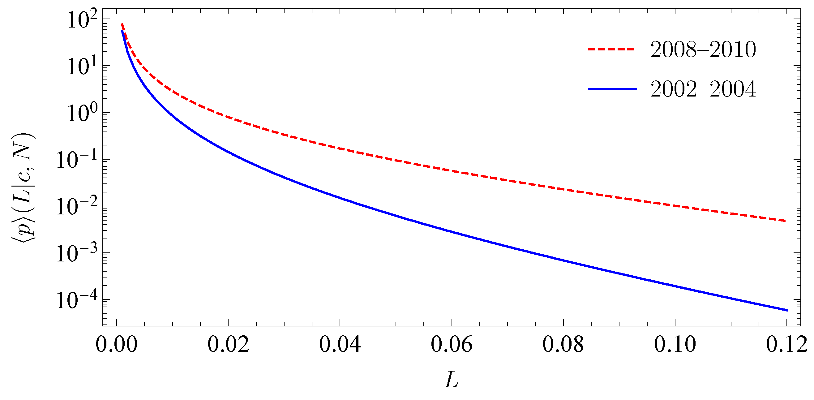
Importantly, we are able to adjust the parameters to different periods, i.e., different market situations. This is a significant feature of the model as the tail of the loss distribution changes for different market situations. The stronger correlations during crises lead to more pronounced tails of the loss distribution. Our model fully grasps this effect. To demonstrate this, we consider two market periods. The first period 2002–2004 is rather calm, whereas the second period 2008–2010 contains the global financial crisis. For simplicity, we solely consider one creditor on one homogeneous market. The empirical results for the period 2002–2004 are $\mu =$ 0.015 month${}^{-1}$, $\rho =$ 0.1 month${}^{-1/2}$, $c=$ 0.3 and for the period 2008–2010 $\mu =$ 0.01 month${}^{-1}$, $\rho =$ 0.12 month${}^{-1/2}$ and $c=$ 0.46. For both periods, we find $N=$ 5, see (Schmitt et al. 2015). In Figure 2, we show the corresponding loss distributions. As anticipated, we find a significantly higher tail in times of crisis.

We estimate the value of the correlations by empirical data. However, the multivariate return distribution (12) that we construct is strongly non-Gaussian and describes the empirical data well. Thus, in the present context copulas, which capture the lower tail dependence, are not needed. However, a comparison with copulas can be found in (Wollschläger and Schäfer 2016).

Moreover, by adjusting the parameter N, we are able to control the strength of the fluctuations around the mean correlation coefficient. The larger the N, the smaller the fluctuations are. In the case $N\to \infty$, the fluctuations are suppressed and the correlation matrix becomes stationary. Hence, the average return distribution (12) becomes a multivariate Gaussian and the benefits of the random matrix approach are not given anymore. The results for the multivariate average portfolio loss distribution in the absence of subordination are

$$\begin{array}{cc}\hfill \underset{N\to \infty }{lim}〈p〉(L|c,N)=& \frac{1}{\sqrt{2\pi }}\underset{-\infty }{\overset{\infty }{\int }}duexp\left(-\frac{u^2}{2}\right)\hfill \\ & \times \frac{1}{\sqrt{det\left(2\pi M_2(u)\right)}}exp\left(-\frac{1}{2}{\left(L-M_1(u)\right)}^{†}{M}_2^{-1}(u)\left(L-M_1(u)\right)\right),\hfill \end{array}$$

(71)

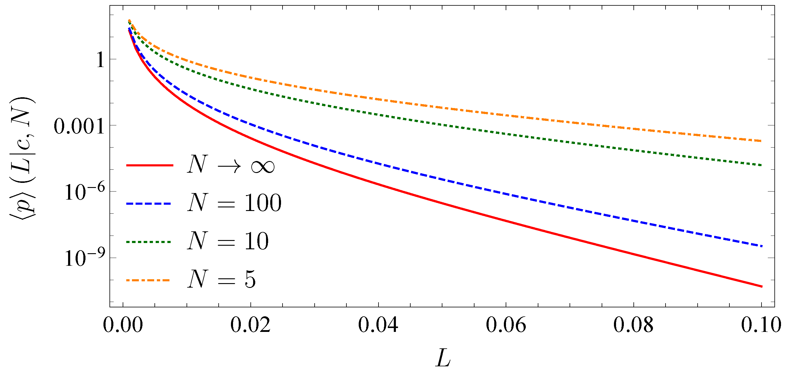
with $M_1(u)=M_1(1,u)$ from (53) and $M_2(u)=M_2(1,u)$ from (54). In Figure 3, we compare the univariate portfolio loss distribution for one creditor on a single homogeneous market and a fixed correlation coefficient of $c=$ 0.3 for different values of N.

The tail of the loss distribution clearly decreases with increasing N. The larger N becomes, the smaller are the outliers of the random correlations around the mean correlation coefficient. This shows the benefit of our random matrix approach compared to standard methods using stationary asset correlations and a multivariate Gaussian for the asset return distribution. Due to the asymmetry of credit risk, outliers that exceed the average correlation coefficient by far have a much stronger impact on the loss distribution than outliers which remain below the average correlation coefficient. This effect is more pronounced for smaller N and leads to an increasing tail.

3.2. One Portfolio, Two Markets

In the following, we use parameters determined by data consisting of 307 stocks that are taken from the S&P500 index traded in the period from 1992 to 2012 (Yahoo n.d.). We find the following empirical results for $T=$ 1 year: $\mu =$ 0.17 year${}^{-1}$, $\rho =$ 0.35 year${}^{-1/2}$, $N=$ 6 and $c=$ 0.28.

We study the impact of investing into two uncorrelated markets. We thus assume two identical uncorrelated markets with the same average correlation coefficient. Furthermore, we assume the empirical parameters to be the same for both markets. The results are shown in Figure 4.

For a comparison, we also show the limiting distribution for only one market $\beta =1$ with the same parameters as in the case of two markets. This distribution is the univariate version of the distribution (66) (see also (Schmitt et al. 2015)). As expected, we see that the diversification, i.e., the separation of the correlation matrix into two blocks leads to a reduction of large portfolio losses. Hence, reducing the risk of large losses can be achieved more effectively by splitting the portfolio onto different uncorrelated markets than by solely increasing the number of credit contracts on one single market. Obviously, this is due to the on-average zero correlations in the off-diagonal blocks. A further reduction of the risk can only be achieved by either splitting the portfolio in more than two markets or investing into markets where the average correlation coefficient is low with little fluctuations. Nevertheless, by increasing the number of uncorrelated markets $\beta$, we obtain for $\beta \to \infty$ the same scenario as in the case of one market with average correlation zero. Here, the diversification effect is limited to the strength of the fluctuations N, where the tail of the loss distribution would only vanish for large N.

This effect has been discussed before, for example, in (Goetzmann et al. 2005), in an empirical setting. We emphasize that we with our results are able to quantitatively model the effect of diversification. According to the adjustability of our model, the benefits of diversification can be modeled for different markets and different market situations.

3.3. Absence of Subordination and Disjoint Portfolios of Equal Size

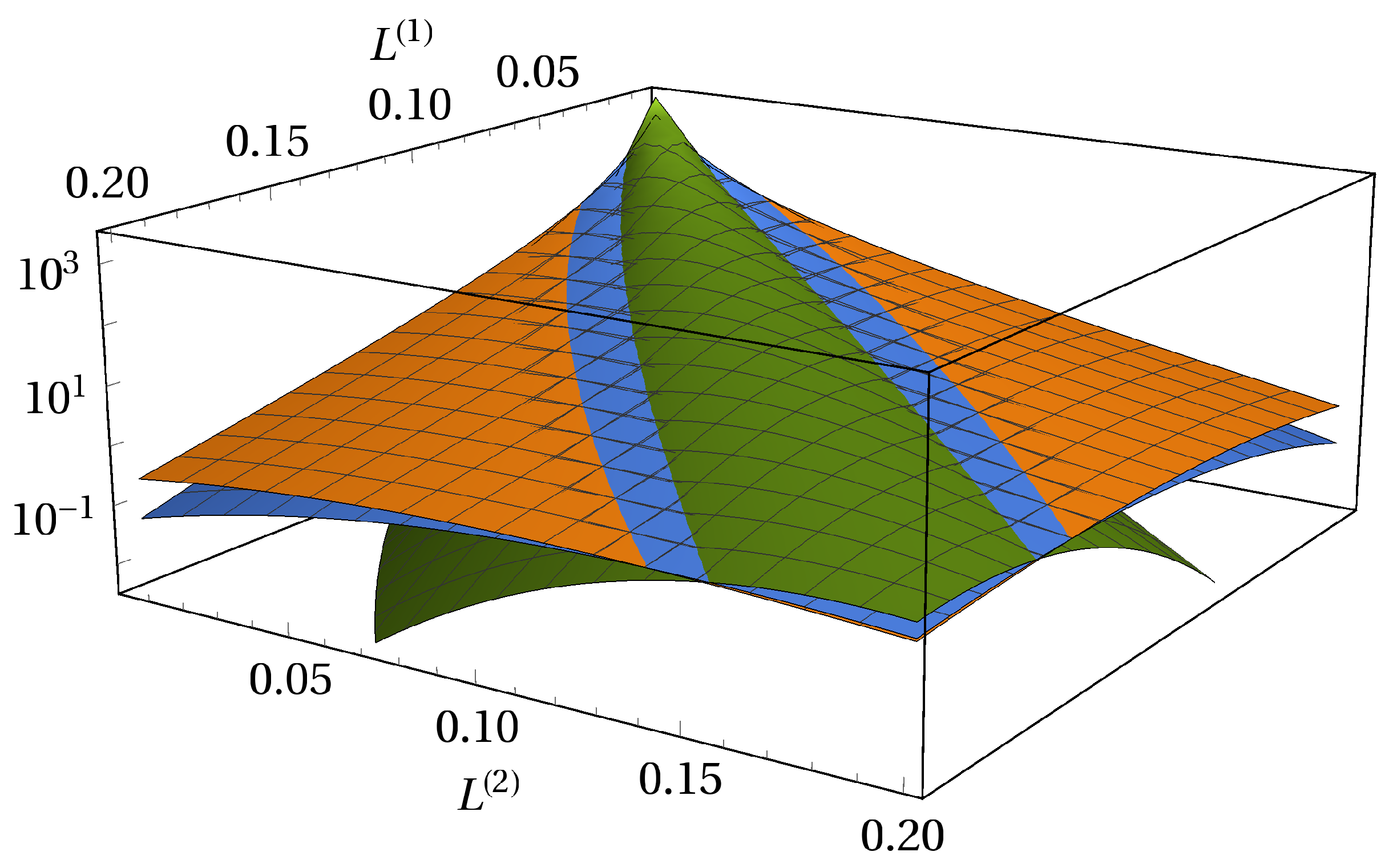
We begin with varying the number of companies K and study the impact on the multivariate loss distribution as well as on the default correlation and the default probabilities. Figure 5 shows the average loss distribution (52) with effective average correlation matrix and homogeneous parameters for two disjoint portfolios of equal size, for different numbers of companies $K=10,20,100$ and empirical values for the parameters.

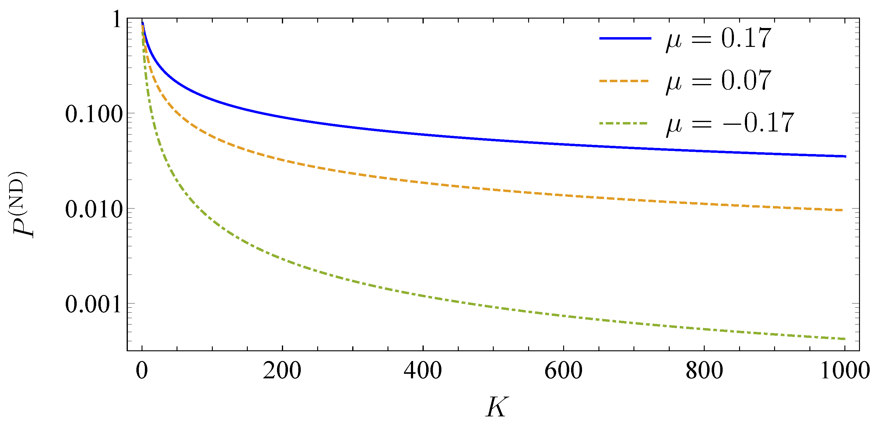
We choose the face value $F_0=75$ and the initial asset value $V_0=100$. The distribution is symmetric. It converges to the limiting distribution (66) as K increases. We thus infer a high correlation of the portfolio losses even for a small number of obligors. The striking peak around the origin $L^{(1)}=L^{(2)}=0$ corresponds to those events that lead to little portfolio loss. This peak arises because of the large drift. Due to the positive drift, the overall number of companies that do not default is larger than the number of companies that default at maturity. Still, this peak does not represent the $\delta$ peak at the origin, which stands for the probability of total survival of all companies. This becomes clear when we calculate the survival probability for all companies. This probability does not depend on whether we have subordinated debt or not and it also does not depend on the composition of our portfolios (see Equation (38)). The effect of different drift parameters $\mu$ is shown in Figure 6.

For every value of $\mu$, the probability of having zero total portfolio loss decreases with an increasing number of companies K. Hence, the weight of the $\delta$ peak on the portfolio loss distribution at $L^{(1)}=L^{(2)}=0$ becomes smaller. This is quite intuitive; the larger the K, the more likely is the default of at least one company.

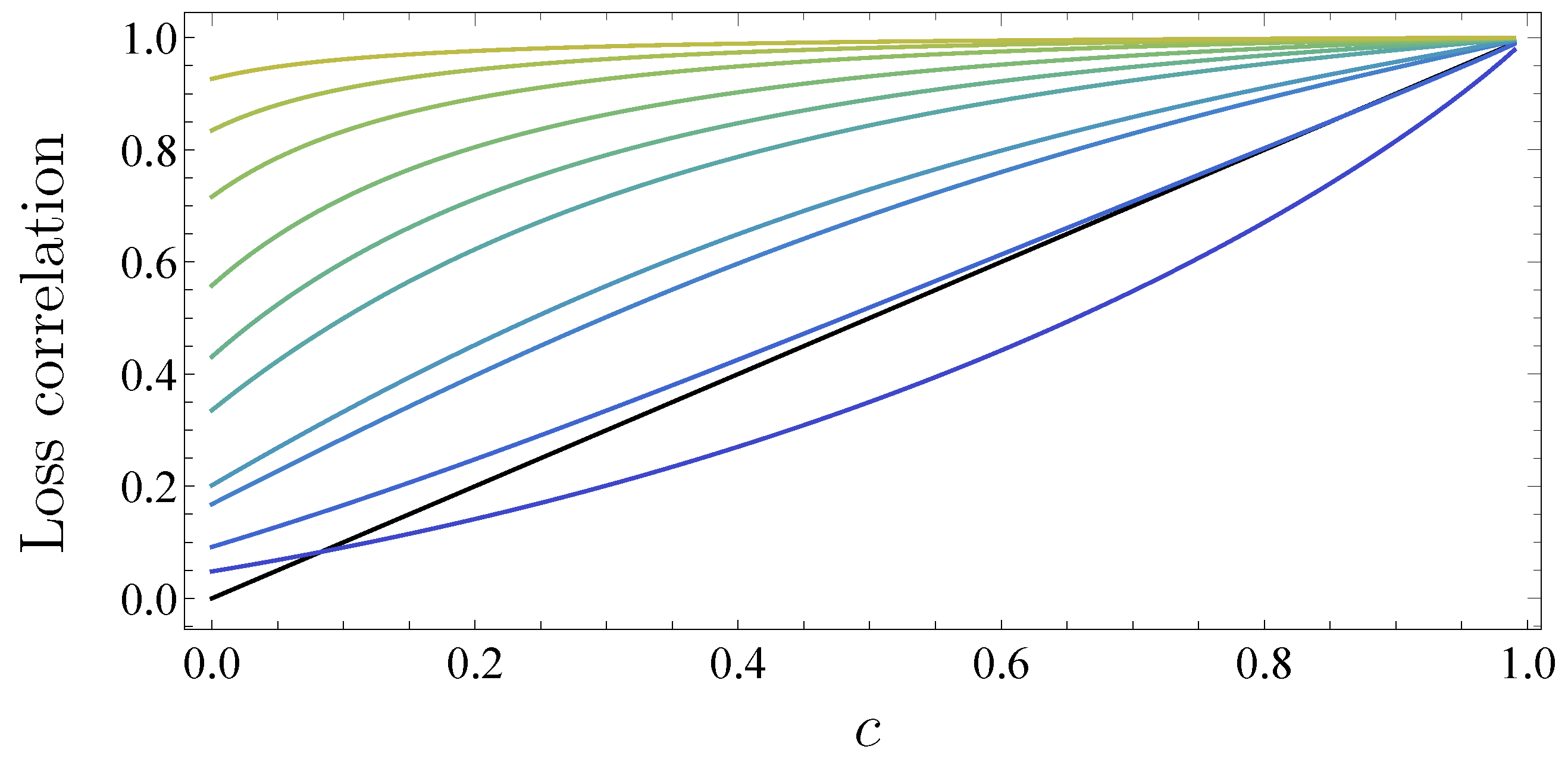
When looking at the portfolio loss correlations, we find large values for little or even zero asset correlation. For a market size of $K=$ 100, i.e., each portfolio is of size 50, we obtain for an average asset correlation of $c=$ 0 a correlation of the portfolio losses of 0.71. This high loss correlation is based on the fact that the asset correlations fluctuate around the mean asset correlation of zero. Due to this fluctuation, we have individual positive and negative correlations. The negative correlations only have a limited effect because the asymmetry of credit risk projects all non defaulting events onto zero while only defaulting events contribute to the loss distribution. Hence, the positive asset correlations dominate the negative ones causing a high portfolio loss correlation. The results are shown in Figure 7.

They are in accordance with the simulation results in (Sicking et al. 2018). The portfolio loss correlation is a monotonic function of the asset correlation c and, for a fixed asset correlation, we find with increasing K an increasing portfolio loss correlation. Depending on the number of companies, the portfolio loss correlation is a convex function (namely, $K=2,4$) or a concave function ($K\ge 8$). However, we emphasize that these results are subject to the second order approximation, which yields better results the larger the K. Large numbers of K lead to very high loss correlations. This confirms that, even without average asset correlation $c=0$, the loss of one large portfolio serves as a forecast for another large portfolio.

3.4. Absence of Subordination and Disjoint Portfolios of Various Sizes

Looking at portfolios of various sizes yields much improved understanding of whether diversification works or not. To analyze this, we consider portfolio one with fixed size $R_1=$ 10 and we consider the overall size of the market $K=$ 30, 110 and the limit $K\to \infty$. In this scenario, the market share of portfolio one will steadily decrease and converge to zero in the limiting case. Hereby, we are able to compare somewhat smaller portfolios with very large ones.

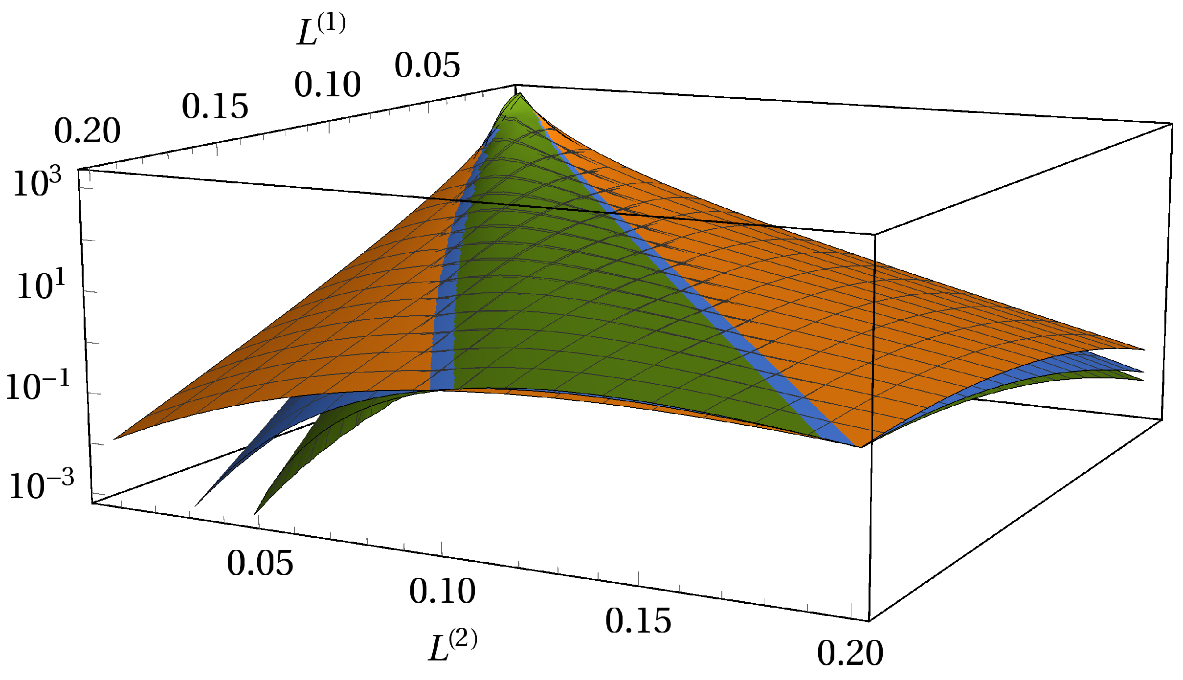
For our calculations, we use the same empirical parameters as in Section 3.3. The effect of different market size K on the loss distribution $〈p〉(L^{(1)},L^{(2)})$ is shown in Figure 8.

There are regions where we have heavy-tailed behavior of the distributions but also others where the distributions decay very fast. In this latter regions that always fulfill the condition $L_1>L_2$, the loss distribution decays considerably faster with increasing market size K. Hence, we find large deviations between the distributions of different market sizes. These deviations only play a minor role because they emerge at a significant low order of the loss distribution. In general, for increasing market size K, the second portfolio describes the market in a better manner. Hence, it is very unlikely for the first portfolio to suffer a big loss in times when the second portfolio of large size exhibits little loss. This explains the fast decay of the loss distribution in the $L_1>L_2$ corner. However, the most important fact is that, along the diagonal $L_1=L_2$ and in the upper corner $L_1<L_2$, significant deviations between the loss distributions for different market sizes do not occur. Here, we also observe heavy-tails of the loss distribution. Especially when we consider the diagonal, we find no deviations and thus no diversification at all. This means that increasing the size of portfolio 2 while keeping the size of portfolio 1 constant does not yield a decrease of concurrent large portfolio losses of equal size. Interestingly, it is more likely to find an event in the upper off-diagonal corner with $L_1<L_2$ than in the lower corner. This can be explained by the fluctuations around the mean correlation coefficient of $c=$ 0.28 and the positive drift $\mu$ = 0.17 year${}^{-1}$. The fluctuations ensure that there is a probability for the assets of portfolio one to be adversely correlated to the assets of portfolio two. Accordingly, there is a significant probability that the small portfolio one suffers no or little default while the second portfolio suffers a major one. This probability decreases when we enlarge the size of portfolio one while keeping the size of portfolio two fixed and still larger than the size of portfolio one. Due to the asymmetry of the portfolio loss distributions regarding the diagonal, we find lower loss correlation for the same market size than in the case of two equal sized portfolios (see Figure 9).

In contrast to two portfolios of equal size, there is a limit correlation of the portfolio losses depending on c in the limit $K\to \infty$. One clearly sees that the limiting curve is reached very quickly for increasing market size. This is due to the fixed size of portfolio one. Increasing its size and the market size would raise the portfolio loss correlation.

3.5. Subordinated Debt

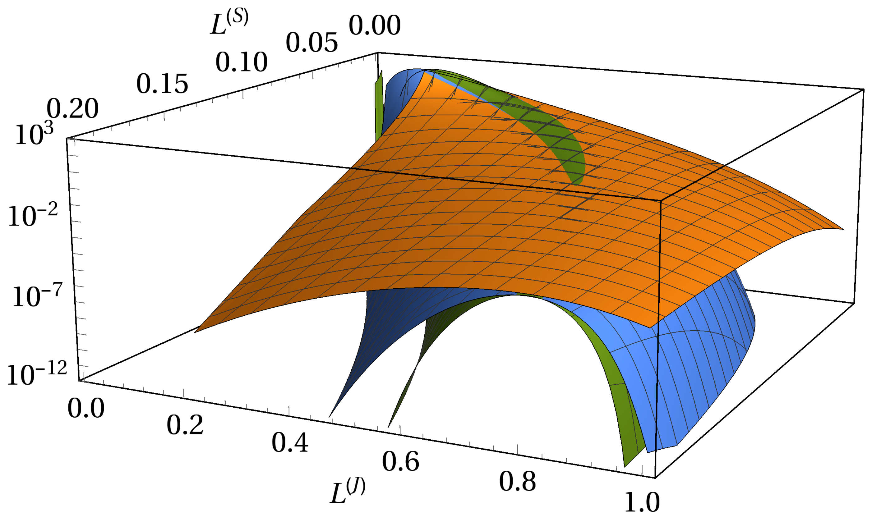
The subordinated debt structure brings a high degree of asymmetry into effect (see Figure 10). We show the joint probability density of two equal-sized portfolios with face values $F_k^{(S)}=$ 37 and $F_k^{(J)}=$ 38. Both senior and junior subordinated creditors operate on the entire market.

The loss of the junior subordinated creditor is always larger or equal than the loss of the senior creditor. We thus have an cutoff along the diagonal line $L^{(S)}=L^{(J)}$. Besides the near region of a curved line, which we define as the back of the distribution, the number of obligors K influences the joint probabilities drastically. Along the back of the distribution, there is almost no deviation between the surfaces of the joint probability densities. Independent of K, the back of the distribution shows heavy tails. Importantly, the curvature reaches for high losses of the junior subordinated creditor evermore to higher losses of the senior creditor. This is an important consequence in times of crisis. When the loss of the junior subordinated creditor becomes extremely large, it is most likely that also the senior creditor suffers a significant loss. Furthermore, we show that, in times of crisis, the majority of an additional loss will be distributed to the senior creditor when there is already a large loss of the junior subordinated creditor.

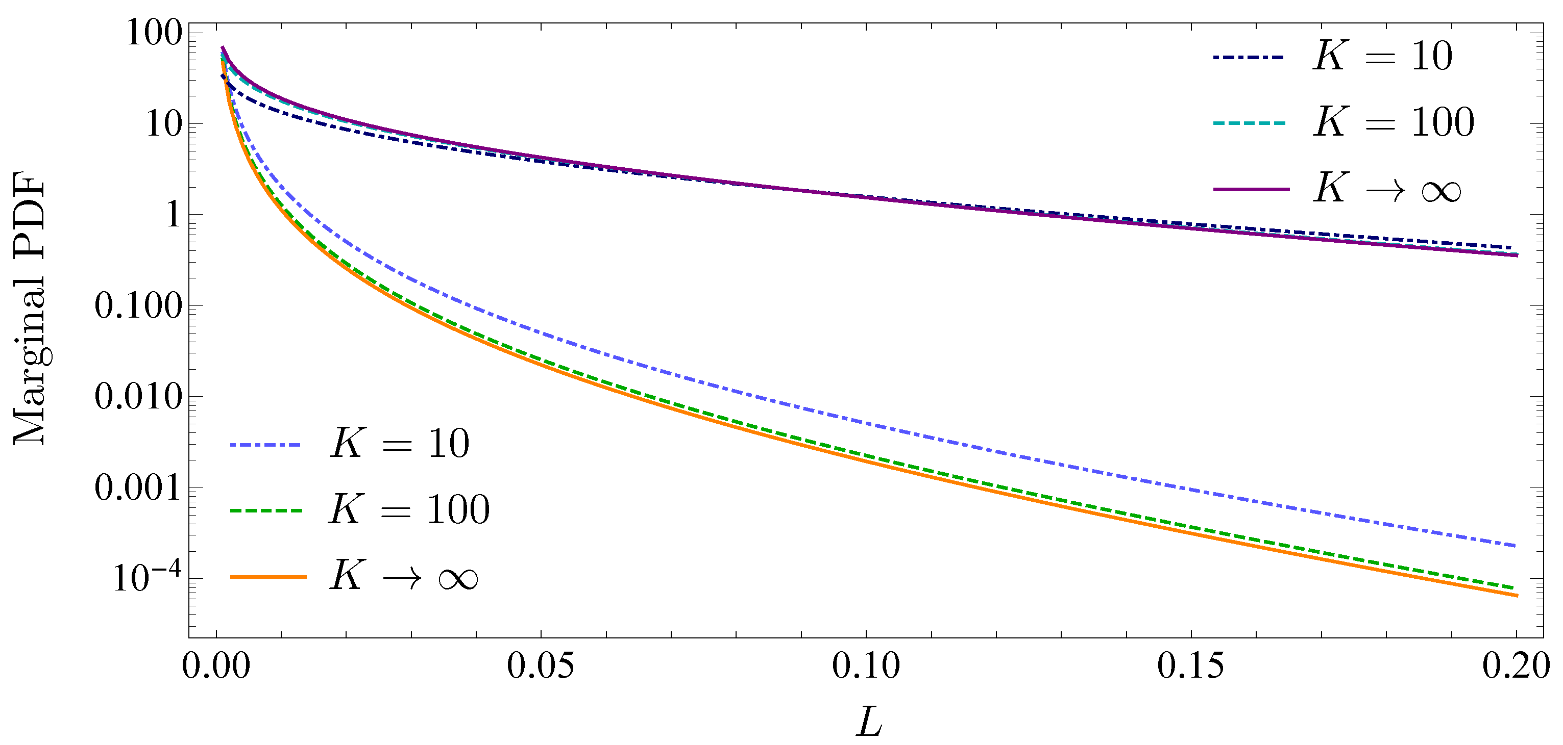
This explains why strong diversification effects do not exist, when we consider the marginal distributions of each creditor (see Figure 11).

The upper three curves belong to the marginal distributions of the junior subordinated creditor and the lower three curves belong to the senior creditor. All distributions show heavy tails and the gap between the senior and junior subordinated creditor enlarges with increasing loss L. The size of this gap becomes smaller when the ratio $F_k^{(S)}/F_k^{(J)}$ becomes larger.

4. Conclusions

Within the Merton model, we calculated a multivariate joint average portfolio loss distribution, taking fluctuating asset correlations into account. We used a random matrix model, which is, most advantageously, analytically tractable and also empirically a good match of stock market data. The multivariate average asset value distribution depends on two parameters only, the effective average asset value correlation and the strength of the fluctuations around this average.

We showed that diversification is achieved much more efficiently by splitting a credit portfolio onto different markets that are, on average, uncorrelated than by solely increasing the number of credit contracts on one single market.

For two non-overlapping portfolios of equal size, we found a symmetric portfolio loss distribution. Studying the portfolio loss correlations, we showed that significant correlations emerge not only for large portfolios containing thousands of credit contracts, but also in accordance with a second order approximation, for small portfolios containing only a few credit contracts. Two non-overlapping portfolios of infinite size have a loss correlation of one and will always suffer the same relative loss.

When we analyzed two non-overlapping portfolios of different size, we found the loss correlations to be limited. Nevertheless, the distributions show heavy tails that make large concurrent portfolio losses likely.

Furthermore, we included subordinated debt, related to CDO tranches. At maturity time, the senior creditor is paid out first and the junior subordinated creditor only if the senior creditor regained the full promised payment. Here, we analytically substantiate that, in case of crisis, i.e., when a large loss of the junior subordinated creditor is highly likely, a large loss of the senior creditor is also very likely. Thus, the concept of subordination does not work as intended in times of crisis. In addition, the marginal distributions show that increasing the size of both portfolios fails to reduce the tail risk significantly.

There are some limitations of our model. Our approach is based on the Merton model, which as discussed in the literature, has some weaknesses (see, e.g., (Duan 1994; Elizalde 2005)). Furthermore, due to the second order approximation in $f_k^{(S)}$ and $f_k^{(J)}$ necessary for analytical tractability, we assume that the face values of all companies are of the same order. Hence, in this approximation, we are not able to analyze the influence of one large company in the loss distribution. Credit default data is very hard to get, implying that we are unfortunately not able to compare the results of our model with empirical data. Nevertheless, our results, when compared to credit risk data in the future, provide an excellent test of the Merton model because we use stock market data for calibration.

The novelty of our approach is the ability to quantitatively model diversification effects that have been mainly qualitatively discussed in the economic literature. Hence, we corroborate qualitative reasoning in the economic literature. Additionally, by obtaining the joint portfolio loss distribution, further quantities such as any kind of risk measure can be calculated.

For further research, it is interesting to analyze avalanche and contagion effects. These effects are included only indirectly in our model, namely by calibrating to stock market states of crisis.

References

- An, Xudong, Yongheng Deng, Joseph B. Nichols, and Anthony B. Sanders. 2015. What is subordination about? Credit risk and subordination levels in commercial mortgage-backed securities (CMBS). The Journal of Real Estate Finance and Economics 51: 231–53. [Google Scholar] [CrossRef]
- Avkiran, Necmi K., Christian M. Ringle, and Rand K. Y. Low. 2018. Monitoring transmission of systemic risk: Application of partial least squares structural equation modeling in financial stress testing. Journal of Risk. [Google Scholar] [CrossRef]
- Bardoscia, Marco, Stefano Battiston, Fabio Caccioli, and Guido Caldarelli. 2017. Pathways towards instability in financial networks. Nature Communications 8: 14416. [Google Scholar] [CrossRef] [PubMed] [Green Version]
- Benmelech, Efraim, and Jennifer Dlugosz. 2009. The alchemy of CDO credit ratings. Journal of Monetary Economics 56: 617–34. [Google Scholar] [CrossRef]
- Bielecki, Tomasz R., and Marek Rutkowski. 2013. Credit Risk: Modeling, Valuation and Hedging. Berlin: Springer Science & Business Media. [Google Scholar]
- Black, Fischer S., and John C. Cox. 1976. Valuing corporate securities: Some effects of bond indenture provisions. The Journal of Finance 31: 351–67. [Google Scholar] [CrossRef]
- Bluhm, Christian, Ludger Overbeck, and Christoph Wagner. 2016. Introduction to Credit Risk Modeling. Boca Raton: CRC Press. [Google Scholar]
- Chava, Sudheer, Catalina Stefanescu, and Stuart Turnbull. 2011. Modeling the loss distribution. Management Science 57: 1267–87. [Google Scholar] [CrossRef]
- Chetalova, Desislava, Thilo A. Schmitt, Rudi Schäfer, and Thomas Guhr. 2015. Portfolio return distributions: Sample statistics with stochastic correlations. International Journal of Theoretical and Applied Finance 18: 1550012. [Google Scholar] [CrossRef]
- Corsi, Fulvio, Stefano Marmi, and Fabrizio Lillo. 2016. When micro prudence increases macro risk: The destabilizing effects of financial innovation, leverage, and diversification. Operations Research 64: 1073–88. [Google Scholar] [CrossRef]
- Crouhy, Michel, Dan Galai, and Robert Mark. 2000. A comparative analysis of current credit risk models. Journal of Banking & Finance 24: 59–117. [Google Scholar]
- Duan, Jin-Chuan. 1994. Maximum likelihood estimation using price data of the derivative contract. Mathematical Finance 4: 155–67. [Google Scholar] [CrossRef]
- Duffie, Darrell, and Kenneth J. Singleton. 1999. Modeling term structures of defaultable bonds. The Review of Financial Studies 12: 687–720. [Google Scholar] [CrossRef] [Green Version]
- Duffie, Darrell, and Nicolae Garleanu. 2001. Risk and valuation of collateralized debt obligations. Financial Analysts Journal 57: 41–59. [Google Scholar] [CrossRef]
- Egloff, Daniel, Markus Leippold, and Paolo Vanini. 2007. A simple model of credit contagion. Journal of Banking & Finance 31: 2475–92. [Google Scholar]
- Elizalde, Abel. 2005. Credit Risk Models II: Structural Models. Documentos de Trabajo CEMFI. Madrid: CEMFI. [Google Scholar]
- Giesecke, Kay, and Stefan Weber. 2004. Cyclical correlations, credit contagion, and portfolio losses. Journal of Banking & Finance 28: 3009–36. [Google Scholar]
- Giesecke, Kay, and Stefan Weber. 2006. Credit contagion and aggregate losses. Journal of Economic Dynamics and Control 30: 741–67. [Google Scholar] [CrossRef]
- Glasserman, Paul. 2004. Tail approximations for portfolio credit risk. The Journal of Derivatives 12: 24–42. [Google Scholar] [CrossRef]
- Glasserman, Paul, and Jesus Ruiz-Mata. 2006. Computing the credit loss distribution in the Gaussian copula model: A comparison of methods. Journal of Credit Risk 2: 33–66. [Google Scholar] [CrossRef]
- Goetzmann, William N., Lingfeng Li, and K. Geert Rouwenhorst. 2005. Long-term global market correlations. Journal of Business 78: 1–38. [Google Scholar] [CrossRef]
- Gorton, Gary, and Anthony M. Santomero. 1990. Market discipline and bank subordinated debt: Note. Journal of Money, Credit and Banking 22: 119–28. [Google Scholar] [CrossRef]
- Hatchett, Jon P. L., and Reimer Kühn. 2009. Credit contagion and credit risk. Quantitative Finance 9: 373–82. [Google Scholar] [CrossRef]
- Heitfield, Eric, Steve Burton, and Souphala Chomsisengphet. 2006. Systematic and idiosyncratic risk in syndicated loan portfolios. Journal of Credit Risk 2: 3–31. [Google Scholar] [CrossRef]
- Hull, John C. 2009. The credit crunch of 2007: What went wrong? Why? What lessons can be learned? Journal of Credit Risk 5: 3–18. [Google Scholar] [CrossRef]
- Humphrey, Jacquelyn E., Karen L. Benson, Rand K. Y. Low, and Wei-Lun Lee. 2015. Is diversification always optimal? Pacific-Basin Finance Journal 35: 521–32. [Google Scholar] [CrossRef]
- Ibragimov, Rustam, and Johan Walden. 2007. The limits of diversification when losses may be large. Journal of Banking & Finance 31: 2551–69. [Google Scholar]
- Itô, Kiyosi. 1944. Stochastic integral. Proceedings of the Imperial Academy 20: 519–24. [Google Scholar] [CrossRef]
- Lando, David. 2009. Credit Risk Modeling: Theory and Applications. Princeton: Princeton University Press. [Google Scholar]
- Lighthill, Michael J. 1958. An introduction to Fourier Analysis and Generalised Functions. Cambridge: Cambridge University Press. [Google Scholar]
- Longstaff, Francis A., and Arvind Rajan. 2008. An empirical analysis of the pricing of collateralized debt obligations. The Journal of Finance 63: 529–63. [Google Scholar] [CrossRef]
- Low, Rand Kwong Yew, Jamie Alcock, Robert Faff, and Timothy Brailsford. 2013. Canonical vine copulas in the context of modern portfolio management: Are they worth it? Journal of Banking & Finance 37: 3085–99. [Google Scholar]
- Low, Rand Kwong Yew. 2017. Vine copulas: Modeling systemic risk and enhancing higher-moment portfolio optimisation. Accounting and Finance. [Google Scholar] [CrossRef]
- Lucas, André, Pieter Klaassen, Peter Spreij, and Stefan Straetmans. 2001. An analytic approach to credit risk of large corporate bond and loan portfolios. Journal of Banking & Finance 25: 1635–64. [Google Scholar]
- Mainik, Georg, and Paul Embrechts. 2013. Diversification in heavy-tailed portfolios: Properties and pitfalls. Annals of Actuarial Science 7: 26–45. [Google Scholar] [CrossRef]
- McNeil, Alexander J., Rüdiger Frey, and Paul Embrechts. 2005. Quantitative Risk Management: Concepts, Techniques and Tools. Princeton: Princeton University Press. [Google Scholar]
- Merton, Robert C. 1974. On the pricing of corporate debt: The risk structure of interest rates. The Journal of Finance 29: 449–70. [Google Scholar]
- Mühlbacher, Andreas, and Thomas Guhr. 2018. Credit risk meets random matrices: Coping with non-stationary asset correlations. Risks 6: 42. [Google Scholar] [CrossRef]
- Münnix, Michael C., Takashi Shimada, Rudi Schäfer, Francois Leyvraz, Thomas H. Seligman, Thomas Guhr, and H. Eugene Stanley. 2012. Identifying states of a financial market. Scientific Reports 2: 644. [Google Scholar] [CrossRef] [PubMed]
- Münnix, Michael C., Rudi Schäfer, and Thomas Guhr. 2014. A random matrix approach to credit risk. PLoS ONE 9: e98030. [Google Scholar] [CrossRef] [PubMed]
- Nitschke, Tobias. 2014. Ensemble-Ansatz zur Modellierung des Kreditrisikos im Falle im Mittel unkorrelierter Märkte. Bachelor’s thesis, University of Duisburg-Essen, Duisburg, Germany. [Google Scholar]
- Sandoval, Leonidas, and Italo De Paula Franca. 2012. Correlation of financial markets in times of crisis. Physica A 391: 187–208. [Google Scholar] [CrossRef] [Green Version]
- Schäfer, Rudi, Markus Sjölin, Andreas Sundin, Michal Wolanski, and Thomas Guhr. 2007. Credit risk—A structural model with jumps and correlations. Physica A 383: 533–69. [Google Scholar] [CrossRef]
- Schmitt, Thilo A., Desislava Chetalova, Rudi Schäfer, and Thomas Guhr. 2013. Non-stationarity in financial time series: Generic features and tail behavior. Europhysics Letters 103: 58003. [Google Scholar] [CrossRef] [Green Version]
- Schmitt, Thilo A., Desislava Chetalova, Rudi Schäfer, and Thomas Guhr. 2014. Credit risk and the instability of the financial system: An ensemble approach. Europhysics Letters 105: 38004. [Google Scholar] [CrossRef] [Green Version]
- Schmitt, Thilo A., Desislava Chetalova, Rudi Schäfer, and Thomas Guhr. 2015. Credit risk: Taking fluctuating asset correlations into account. Journal of Credit Risk 11: 73–94. [Google Scholar] [CrossRef]
- Schönbucher, Philipp J. 2001. Factor models: Portfolio credit risks when defaults are correlated. The Journal of Risk Finance 3: 45–56. [Google Scholar] [CrossRef]
- Schönbucher, Philipp J. 2003. Credit Derivatives Pricing Models: Models, Pricing and Implementation. Hoboken: John Wiley & Sons. [Google Scholar]
- Sicking, Joachim, Thomas Guhr, and Rudi Schäfer. 2018. Concurrent credit portfolio losses. PLoS ONE 13: e0190263. [Google Scholar] [CrossRef] [PubMed] [Green Version]
- Song, Dong-Ming, Michele Tumminello, Wei-Xing Zhou, and Rosario N. Mantegna. 2011. Evolution of worldwide stock markets, correlation structure, and correlation-based graphs. Physical Review E 84: 026108. [Google Scholar] [CrossRef] [PubMed]
- Wagner, Wolf. 2010. Diversification at financial institutions and systemic crises. Journal of Financial Intermediation 19: 373–86. [Google Scholar] [CrossRef]
- Wishart, John. 1928. The generalised product moment distribution in samples from a normal multivariate population. Biometrika 20A: 32–52. [Google Scholar] [CrossRef]
- Wollschläger, Marcel, and Rudi Schäfer. 2016. Impact of nonstationarity on estimating and modeling empirical copulas of daily stock returns. Journal of Risk 19: 1–23. [Google Scholar] [CrossRef] [Green Version]
- Yahoo! n.d. Finance. Available online: http://finance.yahoo.com (accessed on 15 May 2018).
Figure 1.
Schematic visualization of the Merton model. A default occurs if the asset value at maturity drops below the face value . In the red sketched scenario, a default occurs only to the junior subordinated creditor while the senior creditor obtains no loss.
Figure 2.
Average portfolio loss distribution for one creditor with size on a homogeneous market and different periods. The dashed line corresponds to the global financial crisis 2008–2010; the solid line corresponds to the calm period 2002–2004.
Figure 3.
Average portfolio loss distribution for one creditor on a homogeneous market and different values of N.
Figure 4.
Average loss distribution on a logarithmic scale for a different number of markets and market size. The markets are homogeneous and we choose a face value of and the initial asset value .
Figure 5.
Average loss distribution for two disjoint portfolios of same sizes on a logarithmic scale. We show different market sizes, orange, blue and green. The parameters are , , , and a maturity time of .
Figure 6.
Probability of zero portfolio loss depending on the portfolio size K for different drift parameters on a logarithmic scale.
Figure 7.
Portfolio loss correlation on a linear scale depending on the asset correlation c. Both portfolios are homogeneous and have the same size. The market size K ranges from 2 (blue) over 4, 8, 10, 20, 30, 50, 100, 200 to 500 (green). The bisecting line is shown in black.
Figure 8.
Average loss distribution for portfolios of different sizes on a logarithmic scale. Portfolio one is of fixed size and the market size is (orange), (blue) and (green). The parameters are , , , and a maturity time of .
Figure 9.
Portfolio loss correlation as a function of asset correlation c on a linear scale. Portfolio one is of fixed size and the market size K ranges from 30 (blue) over 50, 100, 200 to 500 (green). The limiting curve is shown in black and the bisecting line is shown in red.
Figure 10.
Average portfolio loss distribution of a subordinated debt structure on a logarithmic scale. Both portfolios operate on the entire market. We show different market sizes orange, blue and green.
Figure 11.
Marginal distributions of senior and junior subordinated creditor on a logarithmic scale. The upper three lines belong to the junior subordinated creditor and the lower three lines to the senior creditor.
© 2018 by the authors. Licensee MDPI, Basel, Switzerland. This article is an open access article distributed under the terms and conditions of the Creative Commons Attribution (CC BY) license (http://creativecommons.org/licenses/by/4.0/).
Share and Cite
MDPI and ACS Style
Mühlbacher, A.; Guhr, T. Extreme Portfolio Loss Correlations in Credit Risk. Risks 2018, 6, 72. https://doi.org/10.3390/risks6030072
AMA Style
Mühlbacher A, Guhr T. Extreme Portfolio Loss Correlations in Credit Risk. Risks. 2018; 6(3):72. https://doi.org/10.3390/risks6030072
Chicago/Turabian StyleMühlbacher, Andreas, and Thomas Guhr. 2018. "Extreme Portfolio Loss Correlations in Credit Risk" Risks 6, no. 3: 72. https://doi.org/10.3390/risks6030072
Note that from the first issue of 2016, this journal uses article numbers instead of page numbers. See further details here.