
Reinforcement Learning for Predictive Analytics in Smart Cities

1
Department of Computer Science, University of Thessaly, Papasiopoulou 2-4, Lamia 35100, Greece;
2
School of Computing Science, University of Glasgow, 17 Lilybank Gardens, Glasgow G12 8QQ, UK
*
Author to whom correspondence should be addressed.
Informatics 2017, 4(3), 16; https://doi.org/10.3390/informatics4030016
Submission received: 30 March 2017
/
Revised: 26 May 2017
/
Accepted: 22 June 2017
/
Published: 24 June 2017
(This article belongs to the Special Issue Smart Government in Smart Cities)
Abstract
:The digitization of our lives cause a shift in the data production as well as in the required data management. Numerous nodes are capable of producing huge volumes of data in our everyday activities. Sensors, personal smart devices as well as the Internet of Things (IoT) paradigm lead to a vast infrastructure that covers all the aspects of activities in modern societies. In the most of the cases, the critical issue for public authorities (usually, local, like municipalities) is the efficient management of data towards the support of novel services. The reason is that analytics provided on top of the collected data could help in the delivery of new applications that will facilitate citizens’ lives. However, the provision of analytics demands intelligent techniques for the underlying data management. The most known technique is the separation of huge volumes of data into a number of parts and their parallel management to limit the required time for the delivery of analytics. Afterwards, analytics requests in the form of queries could be realized and derive the necessary knowledge for supporting intelligent applications. In this paper, we define the concept of a Query Controller () that receives queries for analytics and assigns each of them to a processor placed in front of each data partition. We discuss an intelligent process for query assignments that adopts Machine Learning (ML). We adopt two learning schemes, i.e., Reinforcement Learning (RL) and clustering. We report on the comparison of the two schemes and elaborate on their combination. Our aim is to provide an efficient framework to support the decision making of the QC that should swiftly select the appropriate processor for each query. We provide mathematical formulations for the discussed problem and present simulation results. Through a comprehensive experimental evaluation, we reveal the advantages of the proposed models and describe the outcomes results while comparing them with a deterministic framework.
1. Introduction
1.1. Smart Governance and Smart Cities
Smart public governance [1] has been proposed to emphasize the application of information and communication technologies in the public sector and to enhance every technological component realized in Smart Cities (SCs) [2]. SCs should focus on how to reduce the perceived complexity and how citizens will be involved and participate in the SCs management process. Accordingly, public authorities should aim to simplify any interaction in a SC and offer automated services in real time. SCs become smart not only in terms of the way they automate routine functions serving individual persons, buildings, traffic systems but in ways that enable monitoring, understanding, analyzing and planning the city to improve the efficiency, equity and quality of life for its citizens in real time [3]. Such initiatives are based on the collection and the efficient management of the appropriate data to improve the effectiveness of public authorities interventions. Governments and public authorities should decide what data to retrieve, how and their management mechanisms.
In any case, cities should be based on a network of multiple systems all of them being closely connected with citizens’ needs. This perspective requires an integrated vision of a city and its infrastructures [3]. Local authorities should change the way of management of the available infrastructures and be based on automated solutions that will facilitate novel services supporting the so-called vision and leadership [3]. They should also adopt technologies that will secure that efforts in SCs are coordinated rather than isolated. Smart government, hence, has to cope with (a) complexity and (b) uncertainty, thus, has to (c) build competencies and (d) achieve resilience [1]. For many officials, SCs are essentially networks of sensors strewn across the city, connected to computers managing vast flows of data, optimizing urban flows like mobility, waste, crime and money [4]. However, in this aspect, citizens could also participate in the SCs’ infrastructure by adopting the provided services and offer their view in the city by collecting and offering ambient data. A system considering citizens as the part of the provided infrastructure will transform them from passive entities to active towards the facilitation of their lives. Citizens can play an important role not just in the design but also in the delivery of public services. This approach will alleviate the burden of local authorities and reduce the effects of the traditional bureaucratic model of governance as the provided services will be offered in an automatic, de-centralized way. The bureaucratic model is based on government monitoring, thus, citizens have less control over smart initiatives and have a more passive role [3]. In such scenarios, there is the need for building efficient, automated mechanisms that will manage the available data, services and the interaction between citizens and local authorities.
Taking into consideration the huge volumes of data collected by the provided infrastructure and the citizens themselves, it is imperative to propose technologies for managing these data that usually are collected in a ‘distributed’ manner. Data adopted to support innovations can come from a wide range of sources (citizens among them) and stored to different locations (according to the storage management adopted by SCs). Usually, such data are unstructured (they may be the result of services) imposing complexity in the management mechanisms. Efficient decision making on top of the collected data will facilitate any innovation and have significant impact, financial or not, in citizens. The adoption of the appropriate models will allow public authorities to formulate policies, apply strategies and engage citizens in a more efficient way. The envisioned decision making should be automated, provided in real time and cannot be done through the traditional bureaucratic model. The quality and the speed of the decisions play an important role towards the success of the envisioned models. The basic components of decision-making models are analytics services built on top of the collected data. Analytics will give insights on the data and be the basis for supporting high level services offered to the citizens and public authorities.
1.2. Motivation and Research Challenges
The research community has paid increased attention on the large scale data analytics due to their importance in many application domains (SCs among of them). Many cities have proven their intention to become SCs through the adoption of numerous digital devices into their infrastructure. The aim is to have the devices recording ambient information and, afterwards, to manage these data and support intelligent applications that will facilitate citizens’ lives. This data-driven aspect of the management of SCs digital infrastructure aims to make cities knowledgeable and controllable. The aforementioned numerous resources (e.g., sensors, citizens devices) generate huge streams of data. Data can be either processed on-line or stored for future management. In any case, efficient techniques should be applied to support intelligent applications as analytics will be the key for providing the necessary means for the creation of novel as well as efficient decision making mechanisms. Public authorities (e.g., municipalities) will be supported by these mechanisms to derive the optimal decisions related to the services offered to citizens. The most important problem in such scenarios is the efficient management of the huge volumes of the collected data to support decisions in SCs. Large scale data should be ‘integrated’ in the SCs architecture to provide a realistic framework that offers efficient services in citizens and public authorities. The provided services should be concluded in (near) real time on top of automated mechanisms for data collection. As studied (e.g., in [5]), the decision and control management is the most influential component for the realization of a SC. This motivates our work making us to propose a model for the efficient allocation of queries in multiple data partitions. We gain from the separation of data and the parallel execution of queries towards to save time and support real time applications.
As the volumes of the collected data are huge, one efficient approach is to separate them into a number of partitions to facilitate their management and the delivery of analytics. For instance, in a SC, a number of sinks (e.g., servers) could be present in different locations that could be responsible to collect the data originated in different geographical areas. In addition, for storage or performance purposes data could be separated or replicated into a number of servers. Data separation facilitates the parallel processing, thus, it saves time in the generation of responses to the defined queries. An information system should provide immediate and efficient responses to the incoming queries over the huge volumes of data. In this paper, we focus on the support of continuous queries defined by public authorities, citizens or applications. Research efforts in streams query processing [6,7,8,9,10,11,12] focus on the ability of handling incoming data online against a set of continuous queries [13]. We envision that in front of each data partition, a Query Processor () is placed to execute queries over the specific part of data. We do not have any insights about how the data are distributed and we consider a SC dynamic environment where partitions’ contents change over time due to the underlying streams.
The idea of having multiple query processors is motivated by two requirements [14]: (a) when the query volume is too high for a single machine; (b) to ensure continuity of service in case of a query processor failure. Companies like Microsoft [14] or Oracle [15] have already supported the query execution on top of multiple data partitions revealing the need and the practicability of the approach. Hence, for supporting real time applications on top of huge volumes of data, we could rely in the idea of multiple query processors. However, when relying on multiple processors, we need a component that will be responsible for receiving queries and assigning them to a (sub)set of processors and, afterwards, it aggregates the results to return the final response to the application. In this paper, we focus on the former issue, i.e., the conclusion of queries assignments.
We define the concept of Query Controller (), a module that receives queries and secure their efficient execution into the available s. The efficient execution of the incoming queries is related to the best possible assignments i.e., the allocation of each query to a specific where it will be executed. The main research challenge is to determine the most appropriate to maximize the Quality of Result (). The is an indicator that a query response is retrieved in the minimum time and best answers the query. Many methods have been proposed for the evaluation [16,17,18]. The description of the relevant techniques for calculating is beyond the scope of this paper. Without loss of generality, we get . When means that the result is optimal according to the needs of the corresponding query and the opposite stands when .
1.3. Contribution, Research Outcome & Organization
Each assignment, should be concluded by taking into consideration not only the response time and the but also the load of each . We propose the use of Machine Learning (ML) and more specifically the adoption of Reinforcement Learning (RL) [19] and clustering. We focus on the known Q-Learning algorithm and the subtractive clustering. We provide an intelligent mechanism that learns the that best ‘matches’ to each query based on historical data and a set of query families (every query belongs to a query family having specific characteristics). The subsequent step is to create a pool of learners and apply an ensemble learning process, e.g., bagging and boosting [20] to build on top of learners’ advantages and eliminate their disadvantages. Each learning scheme dictates a certain model that is built on top of a set of assumptions [21]. This means that the possible error for each learner comes from different sources according to the adopted assumptions and the defined parameters. The adopted schemes are extended to smoothly be applied in the SC domain and become the basis of the decision making mechanism. In this paper, we extend the model described in [22]. In [22], we propose a similar approach, however, we adopt only the Q-learning algorithm to derive the envisioned assignments. The proposed scheme does not take into consideration the load balancing aspect in the behaviour and does not involve it in the definition of the rewards. In the current effort, we provide two learning schemes (one supervised and an unsupervised) setting up the basis for defining an ensemble learning scheme. We also ‘inject’ into the learners behavior the adoption of multiple parameters (compared to [22]), among them, the load balancing aspect of the ’s behavior. We aim to keep the load of each at low levels, thus, to secure the immediate responses to the incoming queries. The current effort deals with a more complex behavior of the (adoption of multiple parameters) to lead to more efficient assignments, thus, to more efficient analytics. The following list reports on the contribution of our current work:
- we propose two learners responsible to deliver the assignment of queries to a set of s. The first comes from reinforcement learning and the second from clustering;
- we involve in the learning process a set of parameters related to the behaviour of s (e.g., response time, load, ) to be fully aligned with their performance;
- we propose a multiple Q-tables scheme as the knowledge base of the (in the RL case) and a technique for deriving the compactness of the generated clusters (in the clustering case) adopted to deliver the best for each assignment;
- we build on top of an incremental clustering scheme for updating the available clusters;
- we provide a comprehensive performance evaluation of the proposed learning schemes and a comparative assessment with a baseline solution;
- we setup the basis for our next research step where we will rely on a pool of learners and deliver and intelligent scheme for their combination.
The paper is organized as follows. Section 2 discusses research efforts on big data analytics while Section 3 presents our scenario and gives an insight to the adopted architecture. In Section 4, we present our learning schemes and describe the decision process for each one. Model realization, performance metrics, simulation set-up and experimental evaluation are presented in Section 5. Finally, in Section 6, we conclude our paper by giving future extensions.
2. Related Work
In the research community, the efficient management of data streams is significant for many application domains e.g., financial services, life sciences, mobile services. Numerous devices and users create huge volumes of data like environmental data, tweets, social networking interactions or photos [23]. Large scale analytics involves the process of collecting, organizing and analyzing huge volumes of data. Research efforts aim to discover patterns, especially in the case of unstructured data, thus, to extract knowledge and support decision making mechanisms. New functionalities are offered on top of already proposed systems like Hadoop to increase the performance. For instance, the authors in [24] propose Starfish which is a self-tuning tool for large scale analytics. It can be adapted to user requirements and to the system workload in order to provide an efficient solution.
Retrieving a response near real-time could be very difficult due to limitations defined by the amount of data and the underlying hardware performance. Querying data samples and progressive analytics is an efficient solution for the described problem [25]. Samples should be defined taking into consideration the domain, the underlying infrastructure and so on. Specific sampling techniques have been already proposed [26,27,28]. In progressive analytics, the Approximate Query Processing (AQP) technique is the key means for handling the accuracy in early results. AQP aims to provide confidence intervals for early results [26,29,30]. Users are not involved in the process, however, based on the confidence intervals could develop an intelligent mechanism for handling the discussed information. When accuracy is at acceptable levels (according the specific application domain), the process could be stopped.
An analytics system is presented in [31]. The system is based on a framework called Prism and allows users to communicate samples to the system. Queries are processed over the defined samples. The authors proposed Now! a progressive data-parallel computation framework for Windows Azure, where progress is understood as a first-class citizen in the framework. Now! mainly works with streaming engines to support progressive SQL over big data. In [32], the authors present an on-line MapReduce scheme that supports on-line aggregation and continuous queries. For decreasing the latency of the system, the authors propose to have the Map task sending early results to the Reduce tasks. This mechanism enables the generation of approximate results, which is particularly useful for interactive analytics. In [33], the authors present a continuous MapReduce model. The execution of the Map and Reduce functions is coordinated by a data stream processing platform. Latency is improved through a model where mappers are continually fed by data instead of files and the retrieved results are transferred to reducers. CONTROL [27] is an AQP system adopted to support progressive analytics. Users have the opportunity to refine answers and have online control of processing. Hence, users are actively involved in the data analysis process. DBO [34] is another AQP system able to calculate the exact answer to queries over a large relational database in a scalable fashion. DBO can have an insight on the final response together with specific bounds for the accuracy of early results. As more information is processed, the DBO has the opportunity to provide more accurate results. Users can stop the process at any time, if the accuracy level is of their preference.
Large scale data play an important role in decision making models adopted by governments and enterprises. The growth of volume of real-time data requires new techniques and technologies to discover the insight value [35]. Large scale data requires real-time data-intensive processing that runs on high-performance clusters [36]. Apart from ‘static’ data, researchers focus also on the management of large scale data streams [37]. A technique, widely adopted for extracting knowledge from data streams, is clustering. A special case is represented by so-called graph-shaped data (big) streams, which are produced by graph sources providing both structure-and content-oriented knowledge [37]. The parallel management of multiple data partitions gains interest as it offers many advantages. The parallel processing saves time and increases efficiency. In general, the distributed data processing and the aggregation of the results in a centralized authority will increase efficiency especially in the integration of massive multivariate data [38]. The role of large scale data and analytics in SCs has already been revealed in various research efforts [39,40,41,42]. Some of the potential uses of analytics are the Smart Grid, waste management, traffic management, environmental monitoring, security, planning, and so on. The authors in [40] discuss and compare different definitions of the smart city and big data and explores the opportunities, challenges and benefits of incorporating big data applications for smart cities. In addition they attempts to identify the requirements that support the implementation of big data applications for smart city services. The vision of a SC is to improve livability, preservation, revitalization, and attainability of a community [42]. In [40], the authors identify the benefits of the adoption and management of analytics in SCs: (i) efficient resource utilization; (ii) better quality of life; (iii) higher levels of transparency and openness. In general, the services built on top of the provided analytics facilitate the easiest management and control of the different smart city aspects and applications. The processing becomes automated setting up the basis for defining intelligent applications that will facilitate citizens’ lives. Many sectors of the society can gain from large scale data and their management. This information needs to be properly stored and be readily available [43]. Two of the proposed models that adopt large scale data processing in SCs are as follows. In [44], an approach for enabling the ‘easier’ composition of real-time data processing pipelines in SCs is presented, exploiting a block-based design approach, similar to the one adopted in the Scratch programming language for elementary school students. In [5], the authors propose a framework that operates on three levels: data generation and acquisition level collecting heterogeneous data related to SC operations, data management and processing level that filters, analyzes, and stores data to make decisions and events autonomously, and application level initiating execution of the events corresponding to the received decisions.
The concept of an entity executing continuous queries over large scale data has been already explored. In [45] the goal is to recur queries, repeatedly being executed for long periods of time over evolving high-volume data. The proposed Redoop system consists of an extension of Hadoop that pushes the support and optimization of recurring queries into Hadoop’s core functionality. Other systems are Haloop [46], Twister [47] and Nova [48]. Haloop is a modified version of the Hadoop MapReduce framework designed to serve applications. It extends MapReduce with programming support and improves efficiency by making the task scheduler loop-aware and by adding various caching mechanisms. Twister is a programming model that enhances MapReduce and supports iterative query computations. Nova deals with data in large batches using disk-based processing. It fits for a large fraction of data processing use-cases on top of continually-arriving data. Finally, ML is widely used for supporting ‘big data’ tools. The interested reader could refer in [49,50], for a survey on the ML techniques adopted in large scale analytics.
In this paper, we focus on the first step in a decision process i.e., the assignment of each query into a (sub-)set of the available s. We propose two ML schemes for assigning queries under the rationale that a is not the appropriate processor for any arbitrary query. The can have access on historical data related to the performance of the s. The response time, the or the load of each could be some of the parameters that could affect the assignment process. The aim is to gain from s exhibiting high performance and avoid congestions to efficiently support large scale analytics. We propose the adoption of two learning schemes based on ML that derive the QP to which each query should be assigned. We compare their performance and present their advantages and disadvantages. The two schemes could be easily combined in order to support an ensemble learning scheme e.g., a weighted scheme. In the first place of our research agenda is the definition of an efficient combination scheme. The combination scheme will build on top of a pool of different types of learners and adopt a scheme that smoothly aggregates their advantages. The difference of our work compared to other efforts in the field is that we do not focus on the management of the collected data but in the selection of the entities that will manage the data. We do not deal with data generation and acquisition as well as with data filtering and analyzing. These issues are managed by the s that are selected by the . Hence, our model can be considered as complementary to the efforts present in the domain of data management in SCs.
3. Rationale and Preliminary
In Figure 1, we depict the envisioned architecture. Data retrieved in a SC arrive in high rates through a number of streams. We consider that data are stored (either partially or the entire set) and processed at a later stage. A Real Time Processing Engine () is the module that undertakes the responsibility of managing the incoming data. The description of the is beyond the scope of this paper. As the data are collected, they are separated or replicated into a number of partitions. Data parallelism can offer advantages in the ‘efficient’ query execution by splitting the data in to the partitions. We consider that no specific algorithm is adopted for splitting the data and, thus, we cannot be aware on the contents of each partition. Without loss of generality, we assume that n partitions are available. In a large scale data setting, n does not affect the volumes of data stored in partitions.
A set of s are available for executing queries. For every partition, a () is responsible to manage the underlying data and return responses to the . The is in the middle between the s and the public authorities/users/applications. We adopt the term ‘users’, in the remaining, to denote public authorities, users or applications issuing queries to the . Queries belong to specific families. A query family is a set of queries having common characteristics and needs in terms of execution. There are families, having specific characteristics. For each family, a specific execution workflow can be assigned maximizing the and minimizing the required execution time. Every time a query arrives, the should decide the best where the should be assigned to. An assignment is the allocation of the query to the . Each has specific characteristics defined by the family where the belongs to. These characteristics are represented by ) and affect the execution of the . According to s characteristics, every should be assigned to the ‘best’ . The term ‘best’ refers to the that will efficiently execute the (in the minimum time and with the best performance). The is the reward that the gains from the assignment .
Recall that exact answers to queries may not be feasible. Hence, the AQP could result the for each partial response during the execution of a query. Let represent the characteristics of while represent the characteristics of . For instance, some of the characteristics of a could be the load, the response time, the consumption of resources, the adopted optimization techniques and so on. At this time, the final selection is affected mainly by that is dynamically updated according to e.g., the current load of the or the amount of data in the jth partition. affects the performance of the that is induced by the ’s family as well. For instance, could not be the appropriate for executing a specific query family. We apply two learning schemes that are based on historical performance values realized by the combination of and . Such historical values are processed by the in order to be always capable of deriving the best assignment. We adopt two ML algorithms: the Q-learning [19] and the subtractive clustering algorithms [51]. Concerning the Q-learning algorithm, the learning process generates a set of tables (i.e., the Q-Tables) one for each , thus, the allocation is aligned with each family’s characteristics. Concerning the clustering algorithm, our mechanism results clusters based on . Based on these two schemes, the derives the proposed by each scheme and this will take part in the final assignment .
4. The Query Assignment Learning Schemes
4.1. Reinforcement Learning
The RL [19] deals with the behaviour of an agent (i.e., the ) that tries to take some actions in an environment while being at some state (defined later) ( is the set of states). Through actions the agent tries to maximize the long-term reward. Hence, it tries to find the appropriate policy, that maps states to actions. Q-learning is an RL variant. The main advantage of this algorithm is its capability to define the expected reward. The algorithm adopts tables to store information related to the rewards that the agent will gain following a policy. The adopts Q-learning to learn how to assign every to . In RL, the focus is on online performance, which involves balancing between exploration and exploitation. The basic RL problem as applied to Markov Decision Processes (MDPs) consists of: (a) a set of environment states , (b) a set of actions and (c) a set of scalar rewards defined in . In our case: (i) is depicted by the available s, thus, ; (ii) is depicted by the selection of a specific ; (iii) rewards are depicted by the set .
We consider a discrete time domain where each time instance t refers to the step of the RL algorithm where the takes a decision and transits from one state to the other i.e., the assignment of the specific query to a specific . At t, the perceives at being in state (assignment) and the set of possible actions (assignments to other s) . It chooses an action and receives from the environment a new state and a reward . It should be noted that the discussed scenario involves a very dynamic environment as the should interact with the available s that serve a set of and, thus, their characteristics are continuously updated. Based on these interactions, the ‘learning enhanced’ should develop a policy which maximizes the realized final reward retrieved by the assignment : where N is the number of parameters considered to define the final reward. It should be noted that rewards are normalized in [0,1]. In addition, is concluded after the classification of to a specific family. For instance, such parameters could include the time required by to execute a query (the lower the time, the higher the reward), the final retrieved by the assignment and so on. For MDPs without terminal states, the following equation holds true: , where is the future reward discount factor. The acts towards a specific goal which involves the selection of the appropriate . The appropriate has specific characteristics involving:
- the time required for deriving the final result (response time - ) as realized by historical values. We can adopt a simple (e.g., average performance values) or a more complex process over these values. It should be noted that could be depicted by the physical time e.g., in milliseconds;
- the retrieved by the also based on historical values. This parameter is affected by the and the . We can adopt any desired algorithm for the realization of the ;
- the minimum number of steps (in the discrete time) required for the selection of the appropriate . As we focus on a query streaming scenario, the serves a huge number of queries and, thus, the assignment process should be concluded in the minimum time;
- the lowest load L in order to minimize the load of the selected s.
The decision process of the consists of the following parts: (i) The training phase. Training is performed over historical values of performance and aims to create the Q-tables; (ii) The assignment phase. The assignment process is based on the Q-tables derived by the training process. In the beginning, the classifies the to a family and, accordingly, ‘checks’ the corresponding Q-table. Based on the values of the corresponding Q-table, the derives the final assignment.
The advantages of the Q-learning algorithm are: (i) it is a model-free algorithm; (ii) it does not assume knowledge of the environment; (iii) it balances exploration and exploitation. In general, the algorithm is appropriate for ‘static’ environments. In our scenario, we adopt the algorithm to immediately result the assignment for each query. The decision mechanism, when Q-tables are ready (i.e., trained), devotes limited number of steps to derive the assignment (refer to [52]), thus, it reduces the required time. In addition, we do not want to design a model from the beginning as the environment is very dynamic and limited efforts deal with modeling queries and processors. However, we can execute the training process of the Q-tables at pre-defined intervals based on the collected historical values to keep the quality of the decisions at high levels. For instance, we could adopt weekly data for training the available tables. Finally, as described in [52], we can reduce the time required for training, thus, to update the Q-tables more frequently.
4.2. The Training Phase
In the training process, the should build a table for each . The reason is that query families have different requirements concerning the characteristics of the s. Figure 2 presents the discussed setting. Actually, the maintains Q-tables trained at pre-defined intervals. For instance, the Q-tables creation could be realized every week when weekly performance data are retrieved for each and for each query family. The creation of the tables is realized off-line.
Let us focus on a single Q-table. Each Q-table has two dimensions. Rows represent the states of the world () and the columns represent actions () that the could take being at every state (i.e., a query family/type - assignment). This means that when the examines the possibility of assigning the query to a , it decides what action will take according to the values of the specific row of the Q-table. This decision could be the assignment (action ) or the transition to another that corresponds to the specific action and consists of the best choice being at the current state.
The number of Q-tables elements is given by the following equation: The information that the takes into consideration to build the discussed Q-tables is:
- the response time (). We actually get the result of a function applied in the historical values;
- the as defined by function applied on the historical values. historical values are recorded by the after concluding past transactions with each ;
- the number of transitions (T). T shows how many transitions the needs to conclude a decision (selection of a );
- the predicted load (L). L is defined as the result of a predictive scheme that indicates the future load for each .
For each parameter, we apply a technique to derive its final value. For instance, the smaller the T is, the greater the reward becomes. This is because the wants to conclude the assignment at the lowest number of steps. In addition, if , and , the tastes high reward as well.
Each Q-table is created adopting the following equation:
where l is the learning rate, r is the reward, is the future reward discount factor, gives values taken from the Q-table ( and are the state - action combinations already present in the Q-table), and and are the state and the action at t, respectively. l indicates when the learning process has reached to the final point (i.e., an acceptable level of learning). l is calculated based on the number of episodes (episodes define the training time) and decreases over time. The reward r is based on four (4) partial rewards: (a) the reward for the , (b) the reward for the , (c) the reward for T, and, (d) the reward for L. It should be noted that the greater the and the results are, the greater the r becomes. We also get a high r for low T and L. A specific episodes number is adopted in the training phase. The training phase aims to the productive creation of the Q-tables. We need a high enough episodes number to build ‘efficient’ Q-tables that perfectly depict the environment of the the agent. The episodes number could be constant, as indicated in the respective literature.
Paying attention to load L (i.e., number of queries executed by a specific ), we adopt a simple technique to derive the future load estimation for each . In the training process, we pay attention on the load of the that represents the current state of the environment compared to the load of the that depicts the next action. For each , we apply a set of predictors (see Section 4.4) and get the future estimation of the load. Predictors are applied on the historical load values as realized through past transactions. From the retrieved results, we eliminate the maximum and the minimum values in order to avoid optimistic or pessimistic estimations. The remaining values are fed to a function which derives the final future load estimation. The simplest form of is the mean function. Accordingly, we assign high reward when the takes an action that leads to the with the minimum future load instead of rewarding the action that corresponds to the with the highest future load. Through a high number of predictors, we aim to secure the incorporation of the heterogeneity of multiple predictors instead of relying on a single method. In addition, by assigning a high reward to the action that leads to a with low load, we, actually, incorporate a ‘load balancing’ mechanism into the training process.
4.3. The Assignment Process
In pre-defined intervals, the executes the RL training process and, thus, is able to have an up-to-date knowledge on the performance of each . The important issue is that the adopting the Q-learning algorithm is able to incorporate the knowledge about the performance of all the s as experienced for each query family. Hence, the is able to decide the best solution at every incoming query and to be adapted, immediately, to changes in queries characteristics. If the training process is executed in minimum intervals, the will have a more efficient decision making mechanism. However, in such cases, there is an increased cost for training. After creating the Q-tables, the is able to conclude assignments. At first, the classifies the query to a family and selects the corresponding kth Q-table. The randomly selects a and tries to conclude the assignment. represents the initial state of the . If the initial state is the jth entity, the buyer looks at the jth row of the Q-table. Based on the values retrieved by the jth row, the is able to choose the maximum value and, thus, to select the action that should follow. This action could be the final assignment of the query to the or the transition to another (i.e., row). The column of the maximum reward represents the action taken in the upcoming step. If the action is represented by the column means that the should assign the to the (current ). If the best action is e.g., the yth column means that the should take the yth action and ‘check’ the yth row. Every transition to the next consists of the best choice at the current state. The process is repeated till the selects the ‘best’ assignment (action ) or no available solution is present. If the best indicated action is to return to a previous visited , the best assignment is not feasible. In such cases, the allocates the to a randomly selected that depicts a fair behaviour for the specific query family (e.g., exhibiting performance over a threshold). The following algorithm presents the aforementioned steps.
As far as the second learning scheme concerns, the selection process is simple. The proposed model selects the exhibiting the highest score. If multiple s exhibit the highest score, more complex techniques could be applied. For instance, the system could result the top-k s according to the defined score. A probabilistic analysis could be also adopted to derive the best selected for the specific query. However, we leave the discussed analysis and the definition of a more complex mechanism as future work.
| Algorithm 1 The assignment process |
|
4.4. The Predictive Phase
The proposed model adopts a predictive scheme to incorporate the load historical data for each into the training phase. To address this problem, we adopt multiple load predictors) to predict the future load. Different predictors could be used for different s to attain adequate heterogeneity in their predictions. The use of different predictors by different s will give us the ‘different’ thinking in our scenario. For each , we, randomly, choose a set of predictors from the pool which depicts the entire set of the available predictors. We consider predictors where . In Table 1, we see the entire list of predictors. The provided list is not exhaustive meaning that, in many cases, we adopt the same predictor with different parameter values. For instance, in , we adopt the cycle predictor with window size equal to 2, 4, 5, and 7. Every takes into consideration the historical data for each and results the future estimation. Hence, is a mapping , where represents historical data for . The final result is the mean of the selected predictors.
4.5. The Clustering Scheme
The RL scheme can exhibit high performance when data are ‘static’. A very dynamic environment will result in huge amount of data and queries leading the RL scheme to assign queries of the same family to the same s. This requires the update of the Q-tables. However, this could be costly when the number of families and s is high. The second proposed scheme involves the adoption of clustering techniques and does not require any training process (unsupervised learning), thus, it can be executed more frequently. We apply multi-dimensional clustering on top of historical data related to the performance of the s (e.g., response time, , load) to derive the possible clusters and their members. Accordingly, as we cannot be sure about the exact performance of each , we focus on the cluster centres and aggregated them based on the compactness of each cluster and its cardinality. The compactness of a cluster is the average distance between members and the (virtual) centroid of the cluster. Hence, a cluster that exhibits high compactness and a high number of members will affect more the final result which depicts the final performance of a over the parameters. The adopted parameters are already described in Section 4.2. From the available clustering techniques, we adopt the subtractive clustering [51] as it does not require the knowledge of the number of clusters in advance. It should be noted that the proposed clustering scheme is adopted for each query family. The performance of a is depicted by various parameters (as defined in the reinforcement learning model); some of them are based on the family type while others are not. For instance, the load of a processor is not dependent on the query family while the response time could be dependent on the query family. Due to the dynamic nature of the proposed scenario (i.e., the load, the , the response time, etc. change over time), queries belonging to the same families could not, probably, be assigned to the same processors.
In subtractive clustering, every data point is consisted by multiple dimensions and a potential degree is defined according to its location to all other points. This potential depends on the Euclidean distance between the examined point and all other points. The point with the highest potential becomes the first cluster centroid and all the potentials for the other points are recalculated. The point with the highest potential becomes the next cluster centroid. The distance of the new candidate cluster center with all the previously defined cluster centroids should fulfill a specific distance condition defined by the algorithm and ensures that cluster centroids will have a minimum distance between them. If this condition is true then the point becomes the next cluster center or else it is rejected and its potential is set to 0. The potential degree for each point is calculated by:
where and x is the data point, M is the number of points, is a constant (usually set to 4) and is the cluster radius. Subtractive clustering is initially applied (e.g., when the starts performing decisions) over the available historical data and derives a set of clusters. For deriving the appropriate for each query, we calculate the score for each based on the provided clusters. For this, we perform an aggregation process over the clusters in order to derive the final values of each parameter under consideration (e.g., response time, , load). The result of the aggregation process is fed to a model to get the final values and, thus, the score of each . The with the highest score is selected to conclude the assignment.
We aggregate the defined clusters based on data fusion and consensus techniques. We focus on the centroids weighted by the compactness and the cardinality of each cluster. Our mechanism, through data fusion, reaches to a consensus based on the linear opinion pool [53] over the cluster centroids. The linear opinion pool is a standard approach adopted to combine experts’ opinion (where in our case an expert refers to a cluster/centroid) through a weighted linear average of these opinions, i.e., the measurements. It is applied when there is a high need for combining conflicting experts’ opinion. The linear opinion pool, actually, provides a belief aggregation methodology. Our aim is to combine single experts’ opinions (i.e., cluster centroids) in order to produce the opinion of the set of clusters. We define specific weights for each cluster to ‘pay more attention’ on its ‘opinion’ and, thus, to affect more the final aggregated result. Since multiple clusters are available, belief aggregation methods are used to derive the final result. Formally, is the aggregation operator, which, in our case, is the weighted linear average of cluster centroids, where is the weight associated with the centroid of cluster such that and . Weights are calculated based on specific characteristics of each cluster. Concerning the compactness of a cluster, the following equation holds true:
where u is a point belonging in the cluster and depicts the coordinates of that point. The lower the compactness is the more compact the cluster becomes. We also consider the number of points (i.e., the cardinality ) of each cluster. The higher the is the better for the cluster as it involves many points, possibly, close to the centroid (especially when the compactness is high - is low). Based on and , we define the validity of each cluster. The validity of a cluster indicates the ‘importance’ of the cluster for the aggregation process based on the compactness and the cardinality. For instance, a cluster including a high number of points and ‘high’ compactness (low ) should affect more the aggregated result for a . The validity is defined as follows:
where
and , are the thresholds over which the compactness and the cardinality of a cluster is considered as negligible. The proposed mechanism pays equal attention on both parameters (i.e., the compactness and the cardinality) to derive the final validity of each cluster.
For each , based on the set of the available validity (i.e., one for each cluster), we derive the final score depicting the performance of the in serving queries belonging to a specific family. At first, we calculate the final values for every parameter taken into consideration (e.g., , , L) based on the derived weights and the cluster centroids. The aim is to derive a final ‘point’ for each that is consisted of specific values for each parameter. Hence, the final ’s ‘point’ is defined by:
with and is the centroid of each cluster. is a unique value derived by incorporating all the clusters centers (recall that we apply multidimensional clustering on top of multiple parameters) being implicitly affected by the query family. From Equation (5), we see that a cluster having high validity affects more the final value of a performance. It should be noted that we consider that all the discussed parameters are in the interval [0,1]. Accordingly, we define the final score for each based on the aforementioned results. The final score is calculated by comparing the parameters with a set of thresholds. We define as the threshold for each parameter (i.e., , , L). When the result derived by the above described process for each parameter is above/below the three (3) pre-defined thresholds, the score is increased by a constant value (e.g., 100), otherwise, it remains at the previous levels.
4.6. The Incremental Clusters Update Process
The clustering process is realized for every and for every query family resulting a set of clusters. In order to keep up-to-date the available clusters, we adopt the second step of the Doubling algorithm [54]. When new historical data are recorded for the examined parameters, our algorithm checks if the new ‘point’ could be incorporated in the available clusters. Our mechanism calculates the minimum distance between the new ‘point’ and the set of the available clusters. If the discussed distance satisfies specific pre-defined conditions, the new historical data are included in an already present cluster. Otherwise, a new cluster is created. The Algorithm 1 presents the pseudo code of the proposed incremental process.
| Algorithm 2 The incremental clustering update |
|
5. Experimental Evaluation
We elaborate on the performance of the proposed learning schemes, the Reinforcement Learning Scheme () and the Clustering Scheme (). We adopt a set of performance metrics and simulate a query streaming environment. The does not know anything about the execution process followed by every however, it maintains historical values related to the response time (), the for each query family and the load (L) of the s.
5.1. Performance Metrics & Simulation Set-up
We report on the performance of the proposed scheme concerning two axes: (i) the training phase and (ii) the assignment process. We define that represents the required time to derive the final Q-tables or the initial clusters. The following equation holds true: where depicts the time required for training the Q-table corresponding to each query family or the time required to provide the initial set of clusters. As , the scheme exhibits the best performance and the opposite stands when .
Concerning the assignment process, we focus on metrics related to the throughput, the minimum , the maximum and the minimum L. We consider the throughput as the amount of the successful queries executed in a specific time interval. We define , that depicts the throughput of the . is defined as follows: where is the queries executed by the and is the assignment time for each i.e., the time required to conclude . depicts the amount of queries executed by the in a time unit. The greater the is, the greater the performance of the proposed models becomes.
and the metrics aim to evaluate the performance of the proposed schemes concerning the . The following equations hold true: , with
and being the response time of a specific . The metric depicts the average response time as realized by the assignments. It stands that ( represents the normalized response time for each derived by historical values) and, thus, when , the proposed scheme exhibits the best performance (the worst performance is realized when ). The metric reveals if the proposed scheme assigns each query to the , among all, having the best performance related to the response time. As , the scheme exhibits the best performance while the case of depicts the worst performance. It should be noted that, in our experiments, the is represented in seconds.
The is evaluated by the metric which is defined by the following equation: . depicts the maximum value that corresponds to a specific where will be assigned to. The higher the is, the higher the tastes. We also define the maximum coverage metric which depicts the coverage of the maximum possible in the set of the available s. The higher the is, the better performance the model exhibits. When (), the model concludes an assignment which is the best among the entire set of the available s. The following equation holds true:
We define the metric depicting the required steps to derive the final assignment . In our experiments, we present the average value for the entire set of simulations. The lower the is (), the better the performance becomes. The following equation holds true: with depicting the steps required for delivering each assignment.
We also propose the adoption of the metric that depicts the load of the selected s. The following equation holds true: with depicting the load of the finally selected . The lower the is, the better for the mechanism. The reason is that in such cases, the mechanisms selects s exhibiting low load which, virtually, acts as a load balancing model in the assignment process.
Finally, we define the metric as follows: where and represents the weights for each metric. The metric aims to reveal the performance of the model taking into consideration the entire set of the examined metrics. The reason is that the needs a mechanism that derives the final result in the minimum time by selecting the best possible for each query. Hence, the should pay attention on the entire set of metrics at the same time and not on just one of them. The lower the is, the better the performance becomes.
We compare the proposed learning schemes, i.e., the and the with a deterministic model . The examines the entire set of the available s and, accordingly, selects the one having the maximum performance. The is the theoretical limit for our models, thus, we consider three cases: (i) the examines the entire set of the available s and assigns the query to that having the minimum ; (ii) the examines the entire set of the available s and assigns the query to that having the maximum ; (iii) the examines the entire set of the available s and assigns the query to that having the minimum L. The exhibits the worst performance concerning the metric and, actually, is the lower limit of the performance for any model that aims to define assignments between queries and s. On the other hand, the exhibits the best performance related to the , , and metrics. For these metrics, the consists of the upper limit of the performance for any model aiming to define assignments between queries and s.
We run a set of simulations for the discussed scenario. Simulations run in an Intel Pentium 3.2 Ghz processor with 4 GB RAM running Windows 7. Our simulator is written in Java and involves classes for queries, processors and clusters. We simulate the reception of multiple queries. When a query arrives, we select its family and accordingly we adopt the defined Q-tables to derive the appropriate processors. The family of each query is randomly selected when the processing of a query starts (in this set of experiments we do not focus on detailed characteristics of each query family). For creating the tables, we focus on three parameters, i.e., the response time, the and the current load. For each processor, we consider random values for each of the parameters based on the Uniform distribution when we produce historical values. We evaluate our model for diverse realizations of n and . For each experiment, we consider the execution of 1000 queries and take results for the , the and the . We consider , and . In our experiments, we get and . In addition, we create a list of random historical values related to the , the and L in the beginning of each experiment. The initial list’s length is 100 while during experiments, we add historical values to a random belonging to a random family. Finally, , and are the average function, the episodes number is 1000 (for the ) and for statistical processing, we consider the , and L as the last (current) value as depicted in the list of historical values (i.e., calculating the values for each metric).
5.2. Performance Assessment
In Figure 3, we present our results for the metric. We see that the training time of the is heavily affected by n. As n increases, the increases as well. When , the training time for the is 11.0 min, approximately. This means that, in case where the n is high, the pays a high cost for the training process making the scheme inappropriate to be frequently initiated. However, if n is stable, the is not affected by . Consequently, the discussed behaviour causes problems in highly dynamic environments where queries and s characteristics change continually. On the other hand, in Figure 4, we see that the requires at most 10.5 s (approximately) to derive the initial set of clusters over the historical values. It should be noted that this process is executed only once before the starts to take assignment decisions. After that, the adopts the incremental clustering update process. In general, the performance is not affected either by n or by . These results are very significant indicating that the clustering process does not mainly affect the performance of the scheme. Hence, the result of the could be combined with the result of the in the sense that the has always up-to-date information while the exhibits the optimality in the assignment process (this conclusion is derived based also on the upcoming discussion).
The exhibits the worst throughput compared to the as presented in Figure 5. The performance of the is affected by the number of steps required to conclude an assignment. Recall that the derives/aggregates clusters information for every and, accordingly, selects the having the highest score. Hence, in the worst case, it requires steps to derive an assignment. This is alleviated by performing the incremental clustering process only when new historical data are present. Re-clustering could be selected in pre-defined intervals (e.g., every week). In addition, the affects the performance of both schemes as low leads to high . The higher the , the lower the becomes. The same observation stands for n. The lower the n is, the higher the becomes.
In Figure 6 and Figure 7, we present our results related to the metric. In general, the results higher than the . The difference is approximately 14% (in average). No safe conclusion could be derived when (Figure 7). In this case, the two schemes exhibit similar behaviour concerning the results apart from the scenarios where . The is favourite to high n as it can efficiently select the best for concluding an assignment. It should be noted that the proposed schemes are evaluated against e.g., the minimum value in the set of available s, however, both models pay attention, equally, to the entire set of parameters and not on a single one. It is obvious that paying attention on a single parameter forces us to adopt the and not a learning scheme that ‘combines’ multiple s and queries characteristics.
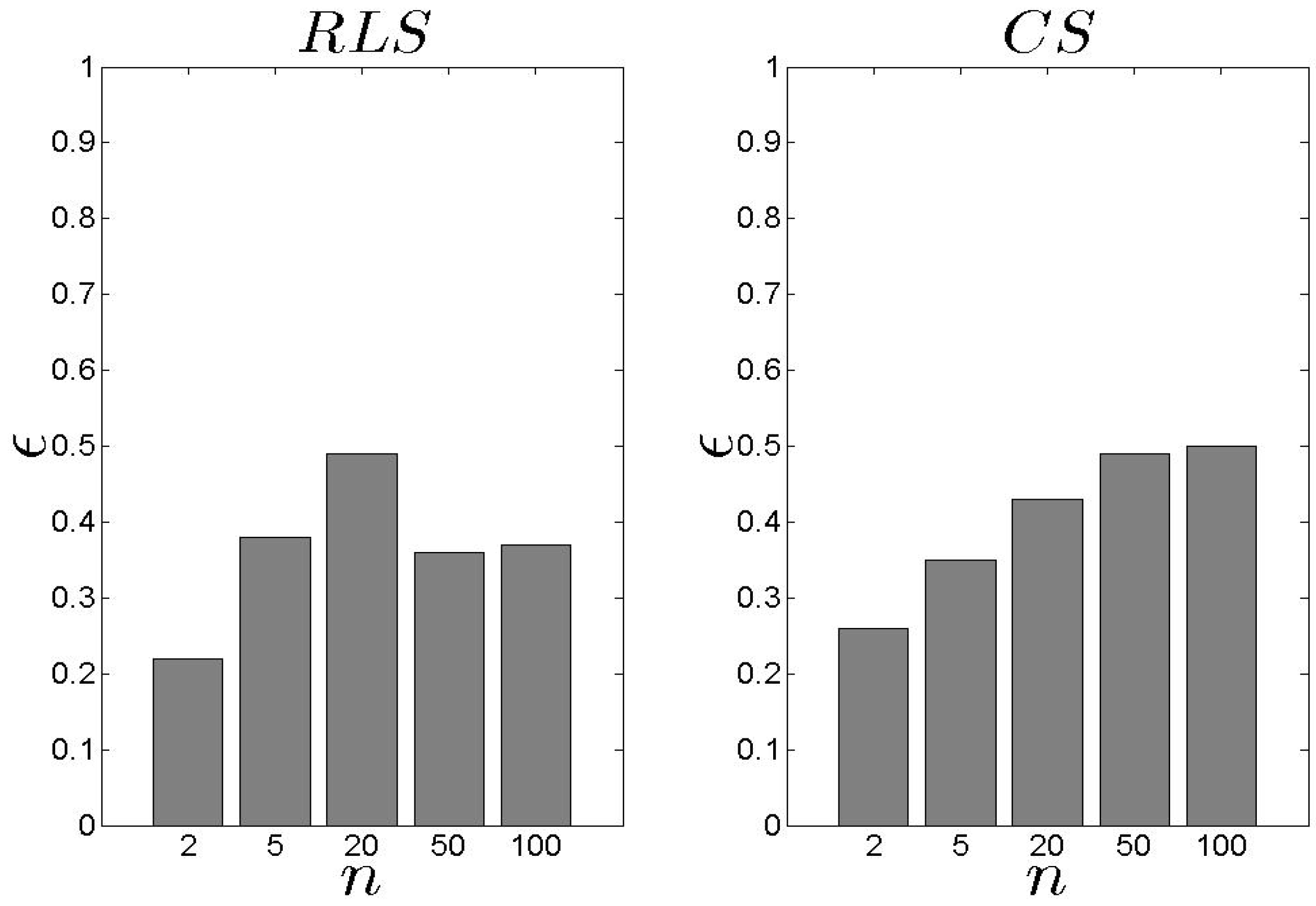
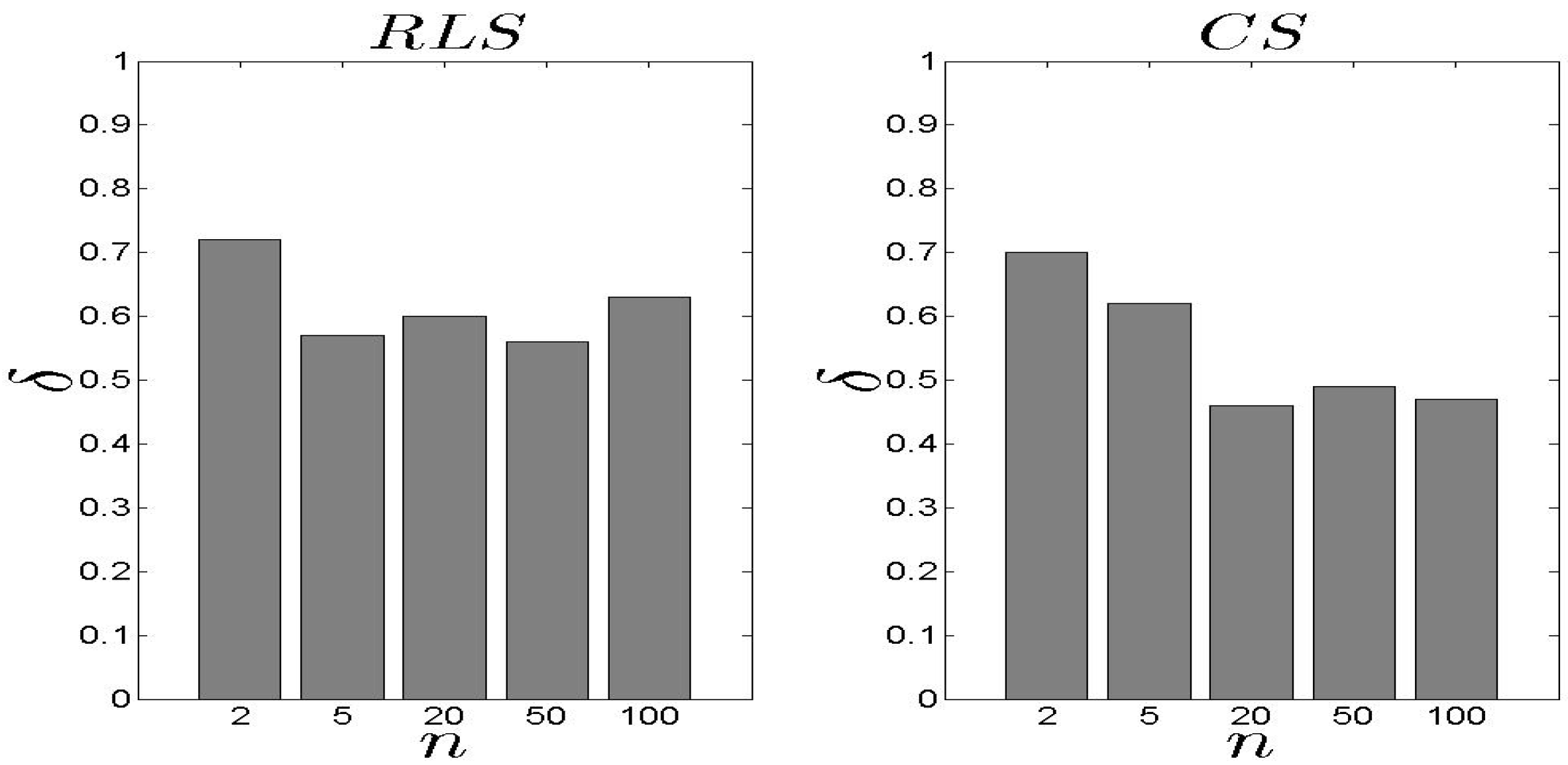
Following the performance related to the metric, the exhibits similar performance as far as the metric concerns (Figure 8 and Figure 9). The behaves worse than the especially when . The average difference is 14% (approximately) while in the case of , the performs better than the when . When , the difference is −14% (approximately) to the favour of the . In general, an average equal to 0.39 for the and 0.40 for the is considered as low, keeping in mind that the proposed schemes select the performing well for the entire set of parameters.
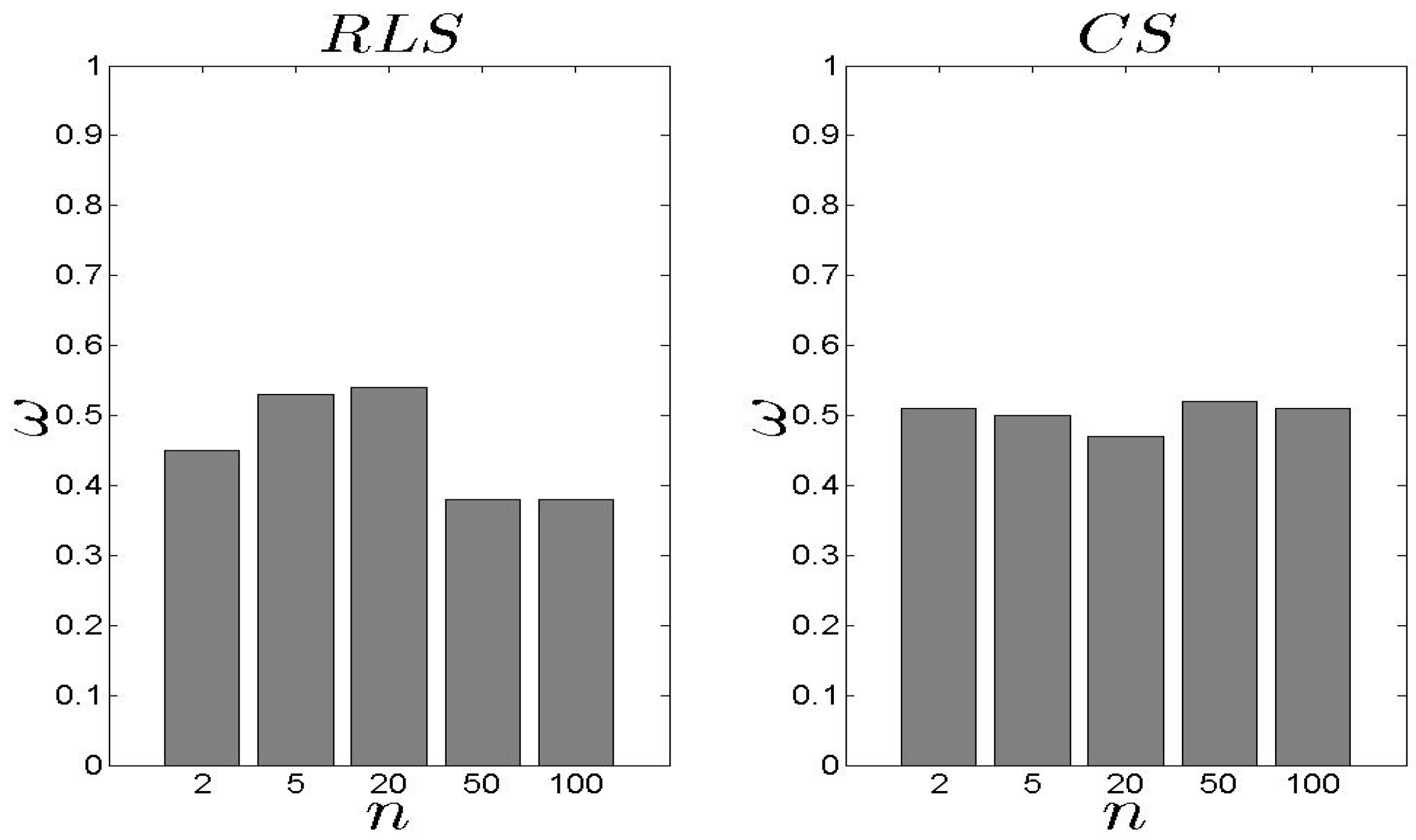
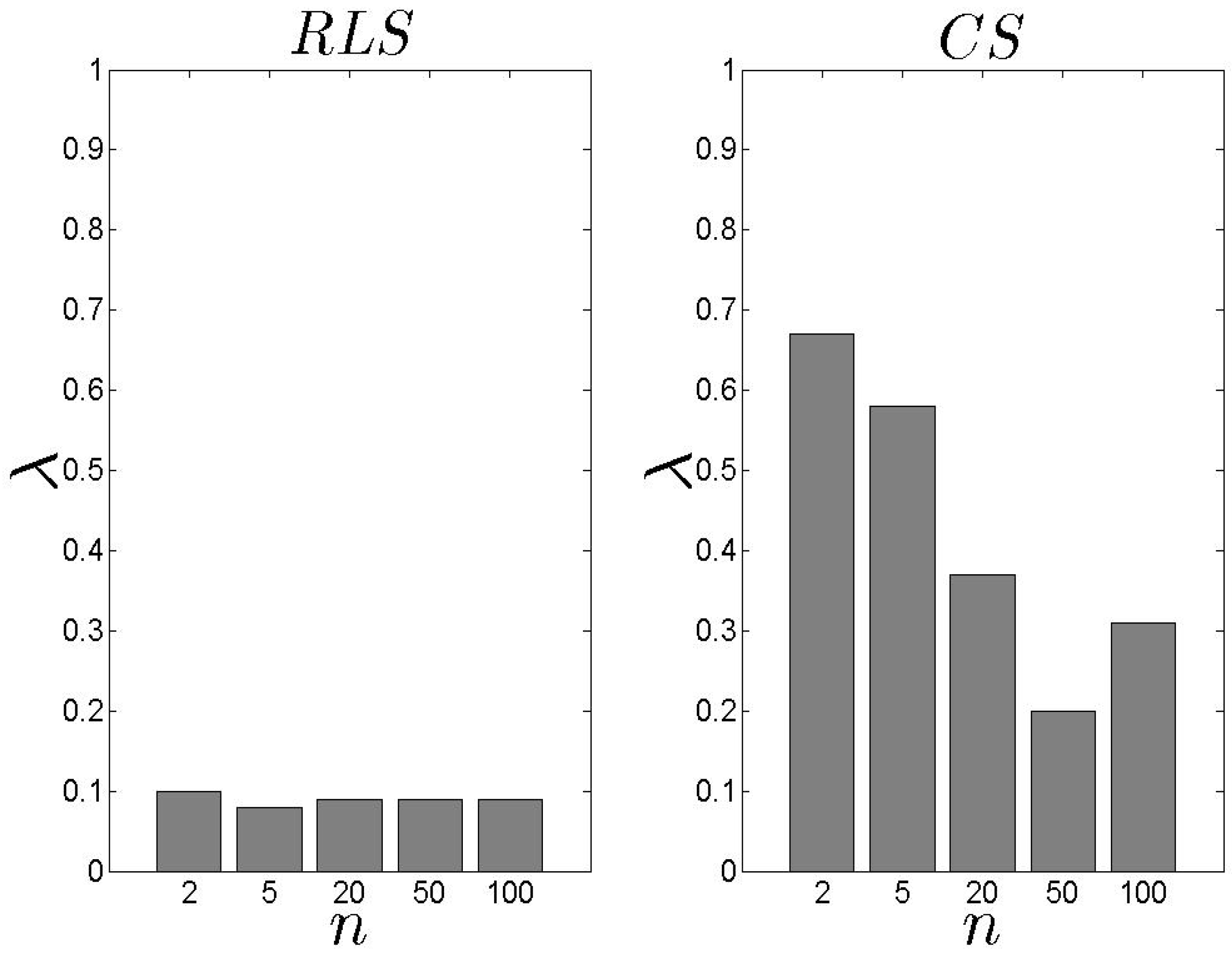
In Figure 10, we present our results related to the metric. Recall that depicts the average achieved by the proposed schemes. We observe that the performs better than the , however, the difference is low. The average is kept close or over 0.6. In addition, as n increases, increases as well which means that high s number lead to high . If we focus on Figure 11 and Figure 12, we observe that both models cover the maximum available when n is low. When n increases, the average increases as well, however, this is not the highest possible value among the entire set of s. The keeps the coverage above 50% for all the experimental scenarios. The average for all the experimental scenarios is 62% and 55% for the and the , respectively.
In Figure 13 and Figure 14, we present our results for the metric. We observe that the difference between the two schemes is significant with the exhibiting an average close to 0.10. In the case, the load of the selected s decreases as the n increases. For high n, the is based on an extensive set of data and, thus, can conclude an efficient s selection. The aforementioned results are not affected by number of families .
The strength of the is depicted by the metric (Figure 15) while its weakness is related to the training time (as already discussed). In Figure 15, we see a comparison between the and the (the has similar performance with the ). The , as , requires more steps to conclude an assignment while the requires only 1.11 steps, in average. This adds a significant burden in the and the , however, both schemes deal with always ‘fresh’ data related to the queries and s characteristics.
We perform an additional comparison between the proposed schemes and the related to the performance for each adopted metric. In Figure 16, we observe that the proposed schemes exhibit difference with the , however, if we take into consideration the entire set of metrics at the same time, our schemes exceed the average, for each one. For instance, it is better to select a that exhibits , and instead of selecting a that exhibits , and . In other words, our schemes aim to s exhibiting acceptable results for the entire set of metrics at the same time and not to s exhibiting the maximum performance to a single metric.
In Table 2, we report on the results related to the metric. In these results, we pay attention on all the examined parameters at the same time. We observe that the outperforms the no matter the number of the available s. These results are mainly affected by the steps required to conclude the assignment. There is a trade off depicted by the up-to-date data considered in the instead of having low assignment time and slightly better performance of the . The advantages of the one become disadvantages of the other. For instance, the exhibits high training time and, thus, in scenarios where n is high, the training process cannot be realized frequently. This stands under the risk of deriving decisions over stale data in highly dynamic environments. However, the leads to the best assignment though the entire set of parameters perspective.
6. Conclusions and Future Work
Smart public governance of Smart Cities should focus on the provision of novel ICT solutions to enhance the adopted technologies. Current Smart Cities initiatives involve the distribution of numerous devices in various locations to create an infrastructure that interacts with its environment. On of the most significant decisions for local authorities is how to manage the huge volumes of data produced by citizens and the underlying infrastructure in real time. Our model is built to support public authorities to create novel applications. We propose and provide the basis for building intelligent applications in Smart Cities, thus, to enhance the smart governance of modern Smart Cities. We define the notion of a Query Controller (), a module that is responsible to handle the incoming queries and decide their assignment to a number of underlying Query Processors (s). We propose two schemes; one that is based on reinforcement leaning and another that is based on clustering. We build on top of the s’ characteristics and provide schemes based on the Q-learning algorithm and the subtractive clustering. The former scheme requires a training process to derive a set of tables adopted to result the appropriate processor for each incoming query. The proposed schemes derive assignments (i.e., queries to processors) taking into consideration a number of parameters. For instance, these parameters can include the response time of each processor for each query family as well as the quality of result () and the load of each . A large set of experiments reveal the efficiency of the proposed model. We focus on the throughput of the when working in a continuous query scenario and on the quality of the final outcome. The training time of the reinforcement learning scheme affects the performance of our model especially when we consider a high number of processors. However, training could not be executed frequently while can be based on techniques that reduce the training time. In addition, our results how that the proposed models can efficiently select the appropriate processor for each query and reduce the required time for returning the final response to the application. We compare our models with a deterministic scheme and show that they perform better than it. Our models take into consideration the entire set of parameters, thus, they efficiently manage the trade-off in the decision making (their decisions are not based on single parameters but in the entire set).
In the first place of our future research agenda is the definition of an adaptive learning model that minimizes the required training time. This gives the opportunity of having multiple initiations of the proposed learning scheme without burdening the performance, thus, alleviating the required effort of local authorities. Another model that efficiently combines the results of the proposed learning schemes is necessary. Such a combination could increase the performance of the . Each scheme derives decisions through a specific perspective. Finally, the definition of a more complex function for deriving the future estimate of the s load is another research issue.
The reason is that a typical average cannot cover the hidden properties in predicting the s load.
Author Contributions
The authors contributed equally to the Cognitive Task Analysis, the representation design, and the writing of the paper.
Conflicts of Interest
The authors declare no conflict of interest.
References
- Scholl, H.; Scholl, M. Smart Governance: A Roadmap for Research and Practice. In Proceedings of the iConference Summary, Berlin, Germany, 4–7 March 2014; pp. 163–176. [Google Scholar]
- Meijer, A.; Bolivar, M. Governing the Smart City: Scaling-Up the Search for Socio-Techno Synergy. In Proceedings of the 2013 EGPA Conference, Scotland, UK, 11–13 September 2013. [Google Scholar]
- Bolivar, M.P.R. Smart Cities: Big Cities, Complex Governance? In Transforming City Governments for Successful Smart Cities; Public Administration and Information Technology 8; Springer International Publishing: Berlin, Germany, 2015. [Google Scholar]
- Kresin, C. Design Rules for Smarter Cities. In ‘Smart Citizens’ Future Everything; Hemmet, D., Townsend, A., Eds.; Future Everything Publications: Manchester, UK, 2013; pp. 51–54. [Google Scholar]
- Silva, B.N.; Khan, M.; Han, K. Big Data Analytics Embedded Smart City Architecture for Performance Enhancement through Real-Time Data Processing and Decision-Making. Wirel. Commun. Mobile Comput. 2017, 2017, 9429676. [Google Scholar]
- Abadi, D.J.; Carney, D.; Cetintemel, U.; Cherniack, M.; Convey, C.; Lee, S.; Stonebraker, M.; Tatbul, N.; Zdonik, S.B. Aurora: A New Model and Architecture for Data Stream Management. VLDB J. 2003, 12, 120–139. [Google Scholar] [CrossRef]
- Arasu, A.; Babcock, B.; Babu, S.; Cieslewicz, J.; Datar, M.; Ito, K.; Motwani, R.; Srivastava, U.; Widom, J. STREAM: The Stanford Data Stream Management System; Part of the series Data-Centric Systems and Applications; Springer: Berlin/Heidelberg, Germany, 2004. [Google Scholar]
- Chandrasekaran, S.; Franklin, M.J.P. Soup: A system for streaming queries over streaming data. VLDB J. 2003, 12, 140–156. [Google Scholar] [CrossRef]
- Cranor, C.; Johnson, T.; Spataschek, O.; Shkapenyuk, V. Gigascope: A Stream Database for Network Applications. In Proceedings of the International Conference on Management of Data and Symposium on Principles Database and Systems (SIGMOD), San Diego, CA, USA, 9–12 June 2003. [Google Scholar]
- Hammad, M.A.; Ghanem, T.M.; Aref, W.G.; Elmagarmid, A.K.; Mokbel, M.F. Efficient Pipelined Execution of Sliding-Window Queries Over Data Streams; Technical Report; Department of Computer Science, Purdue University: West Lafayette, IN, USA, 2003. [Google Scholar]
- Motwani, R.; Widom, J.; Arasu, A.; Babcock, B.; Babu, S.; Datar, M.; Manku, G.S.; Olston, C.; Rosenstein, J.; Varma, R. Query Processing, Approximation, and Resource Management in a Data Stream Management System. In Proceedings of the First Biennial Conference on Innovative Data Systems Research (CIDR), Asilomar, CA, USA, 5–8 January 2003. [Google Scholar]
- Yao, Y.; Gehrke, J. The Cougar Approach to In-Network Query Processing in Sensor Networks. SIGMOD Rec. 2002, 31, 9–18. [Google Scholar] [CrossRef]
- Mokbel, M.; Xiong, X.; Hammad, M.; Aref, W. Continuous Query Processing of Spatio-Temporal Data Streams in PLACE. Geoinformatics 2005, 9, 4. [Google Scholar] [CrossRef]
- Funellblack, Supporting Multiple Query Processors. Available online: https://docs.funnelback.com/more/extra/supporting_multiple_query_processors.html (accessed on 20 March 2017).
- Oracle Parallel Server Concepts and Administration. Available online: https://docs.oracle.com/cd/A58617_01/server.804/a58238/ch1_unde.htm (accessed on 20 March 2017).
- Ciaccia, P.; Patella, M. Approximate Similarity Queries: A Survey; University of Bolognia: Bologna, Italy, 2001. [Google Scholar]
- Ramakrishnan, G.; Uma Maheswari, S. Novel Approach for Predicting Difficult Keyword Queries over Databases using Effective Ranking. Int. J. Eng. Res. Technol. 2015, 4. [Google Scholar] [CrossRef]
- Zhang, W.; Li, J. Processing Probabilistic Range Query over Imprecise Data Based on Quality of Result. In APWeb Workshops; LNCS; Springer: Berlin/Heidelberg, Germany, 2006; pp. 441–449. [Google Scholar]
- Sutton, R.S.; Barto, A.G. Reinforcement Learning: An Introduction; MIT Press: Cambridge, MA, USA, 1998. [Google Scholar]
- Bishop, C. Pattern Recognition and Machine Learning; Springer: Berlin/Heidelberg, Germany, 2009. [Google Scholar]
- Alpaydin, E. Introduction to Machine Learning, 2nd ed.; The MIT Press: Cambridge, MA, USA, 2010. [Google Scholar]
- Kolomvatsos, K.; Hadjiefthymiades, S. Learning the Engagement of Query Processors for Intelligent Analytics. Springer Appl. Intell. J. 2016, 1–17. [Google Scholar] [CrossRef]
- Singh, S.; Singh, N. Big Data Analytics. In Proceedings of the International Conference on Communication, Information, Computing Technology, Mumbai, India, 19–20 October 2012. [Google Scholar]
- Herodotou, H.; Lim, H.; Luo, G.; Borisov, N.; Dong, L.; Cetin, F.B.; Babu, S. Starfish: A Self-tuning System for Big Data Analytics. In Proceedings of the Biennial Conference on Innovative Data Systems Research (CIDR), Asilomar, CA, USA, 9–12 January 2011. [Google Scholar]
- Agarwal, S.; Milner, H.; Kleiner, A.; Talwalkar, A.; Jordan, M.; Madden, S.; Mozafari, B.; Stoica, I. Knowing When You’re Wrong: Building Fast and Reliable Approximate Query Processing Systems. In Proceedings of the ACM SIGMOD Conference, Snowbird, UT, USA, 22–27 June 2014. [Google Scholar]
- Chaudhuri, S.; Das, G.; Srivastava, U. Effective use of block-level sampling in statistics estimation. In Proceedings of the 2004 ACM SIGMOD international conference on Management of data, Paris, France, 13–18 June 2004. [Google Scholar]
- Hellerstein, J.M.; Avnur, R. Informix under control: Online query Processing. Data Min. Knowl. Discov. J. 2000, 4, 281–314. [Google Scholar] [CrossRef]
- Pansare, N.; Borkar, V.R.; Jermaine, C.; Condie, T. Online aggregation for large MapReduce jobs. In Proceedings of the 37th International Conference on Very Large Data Bases (VLDB), Seattle, WA, USA, 29 August–3 September 2011. [Google Scholar]
- Doucet, A.; Briers, M.; Senecal, S. Efficient block sampling strategies for sequential Monte Carlo methods. J. Comput. Graphical Stat. 2006. [Google Scholar] [CrossRef]
- Raman, V.; Raman, B.; Hellerstein, J.M. Online dynamic reordering for interactive data processing. In Proceedings of the 25th International Conference on Very Large Data Bases (VLDB), Scotland, UK, 7–10 September 1999. [Google Scholar]
- Chandramouli, B.; Goldstein, J.; Quamar, A. Scalable Progressive Analytics on Big Data in the Cloud. Proc. VLDB Endow. 2013, 6, 1726–1737. [Google Scholar] [CrossRef]
- Condie, T.; Conway, N.; Alvaro, P.; Hellerstein, J.M.; Elmeleegy, K.; Sears, R. MapReduce online. In Proceedings of the 7th Conference on Networked Systems Design and Implementation, San Jose, CA, USA, 28–30 April 2010. [Google Scholar]
- Logothetis, D.; Yocum, K. Ad-hoc Data Processing in the Cloud. Proc. VLDB Endow. 2008, 1, 1472–1475. [Google Scholar] [CrossRef]
- Jermaine, C.; Arumugam, S.; Pol, A.; Dobra, A. Scalable approximate query processing with the DBO engine. In Proceedings of the ’07 International Conference on Management of Data (SIGMOD), Beijing, China, 11–14 June 2007. [Google Scholar]
- Bakhtiar, A.; Joan, L. Sketch of Big Data Real-Time Analytics Model. In Proceedings of the The Fifth International Conference on Advances in Information Mining and Management, Brussels, Belgium, 21–26 June 2015. [Google Scholar]
- Vennila, V.; Kannan, A.R. Symmetric Matrix-based Predictive Classifier for Big Data computation and information sharing in Cloud. Comput. Electr. Eng. 2016, 56, 831–841. [Google Scholar] [CrossRef]
- Hassani, M.; Spaus, P.; Cuzzocrea, A.; Seidi, T. I-HASTREAM: Density-Based Hierarchical Clustering of Big Data Streams and Its Application to Big Graph Analytics Tools. In Proceedings of the 16th IEEE/ACM International Symposium on Cluster, Cloud and Grid Computing, Cartagena, Colombia, 16–19 May 2016. [Google Scholar]
- Ma, S.; Liang, Z. Design and Implementation of Smart City Big Data Processing Platform Based on Distributed Architecture. In Proceedings of the 10th International Conference on Intelligent Systems and Knowledge Engineering (ISKE), Taipei, Taiwan, 24–27 November 2015. [Google Scholar]
- Arasteh, H.; Hosseinnezhad, V.; Loia, V.; Tommasetti, A.; Troisi, O.; Shafie-khah, M.; Siano, P. IoT-based Smart Cities: A Survey. In Proceedings of the IEEE 16th International Conference on Environment and Electrical Engineering (EEEIC), Florence, Italy, 6–8 June 2016. [Google Scholar]
- Eiman, A.N.; Hind, A.N.; Nader, M.; Jameela, A.J. Applications of big data to smart cities. J. Internet Ser. Appl. 2015, 6, 25. [Google Scholar]
- Kumar, S.; Prakash, A. Role of Big Data and Analytics in Smart Cities. Int. J. Sci. Res. 2016, 5, 12–23. [Google Scholar]
- Sun, Y.; Song, H.; Jara, A.; Bie, R. Internet of Things and Big data Analytics for Smart Cities and Connected Communities. IEEE Access 2016, 4, 766–773. [Google Scholar] [CrossRef]
- Spatti, D.H.; Bartocci Lobini, L.H. Computational Tools for Data Processing in Smart Cities. In Smart Cities Technologies; InTech: Rijeka, Croatia, 2016. [Google Scholar]
- Bonino, D.; Rizzo, F.; Pastrone, C.; Soto, J.A.C.; Ahlsen, M.; Axling, M. Block-based realtime big-data processing for smart cities. In Proceedings of the IEEE International Smart Cities Conference (ISC2), Trento, Italy, 12–15 September 2016. [Google Scholar]
- Lei, C.; Zhuang, Z.; Rundensteiner, E.A.; Eltabakh, M. Redoop Infrastructure for Recurring Big Data Queries. In Proceedings of the 40th International Conference on very Large Data Bases (VLDB), Hangzhou, China, 1–5 September 2014. [Google Scholar]
- Bu, Y.; Howe, B.; Balazinska, M.; Ernst, M.D. The HaLoop approach to large-scale iterative data analysis. VLDB J. 2012, 21, 169–190. [Google Scholar] [CrossRef]
- Ekanayake, J.; Li, H.; Zhang, B.; Gunarathne, T.; Bae, S.-H.; Qiu, J.; Fox, G. Twister: A runtime for iterative mapreduce. In Proceedings of the 19th ACM International Symposium on High Performance Distributed Computing, Chicago, IL, USA, 21–25 June 2010; pp. 810–818. [Google Scholar]
- Olston, C.; Chiou, G.; Chitnis, L.; Liu, F.; Han, Y.; Larsson, M.; Neumann, A.; Rao, V.B.N.; Karasubramanian, V.; Seth, S.; et al. Nova: continuous pig/hadoop workflows. In Proceedings of the SIGMOD Conference, Athens, Greece, 12–16 June 2011; pp. 1081–1090. [Google Scholar]
- Al-Jarrah, O.Y.; Yoo, P.D.; Muhaidat, S.; Karagiannidis, G.K.; Taha, K. Efficient Machine Learning for Big Data: A Review. Big Data Res. 2015, 2, 87–93. [Google Scholar] [CrossRef]
- Zhou, L.; Pan, S.; Wang, J.; Vasilakos, A.V. Machine learning on big data: Opportunities and challenges. Neurocomputing 2017, 237, 350–361. [Google Scholar] [CrossRef]
- Jang, J.-S.R.; Sun, C.T.; Mizutani, E. Neuro-Fuzzy and Soft Computing—A Computational Approach to Learning and Machine Intelligence; Prentice Hall: Upper Saddle River, NJ, USA, 1997. [Google Scholar]
- Boulougaris, G.; Kolomvatsos, K.; Hadjiefthymiades, S. Building the Knowledge Base of a Buyer Agent Using Reinforcement Learning Techniques. In Proceedings of the 2010 IEEE World Congress on Computational Intelligence (WCCI 2010), IJCNN, Barcelona, Spain, 18–23 July 2010; pp. 1166–1173. [Google Scholar]
- Manyika, J.; Durrant-Whyte, H. Data Fusion and Sensor Management: A Decentralized Information-Theoretic Approach; Ellis Horwood: New York, NY, USA; London, UK, 1994. [Google Scholar]
- Charikar, M.; Chekuri, C.; Feder, T.; Motwani, R. Incremental clustering and dynamic infomation retrieval. In Proceedings of the ACM 29th Annual Symposium on Theory of Computing, El Paso, TX, USA, 4–6 May 1997. [Google Scholar]
Figure 1.
The architecture of our model.
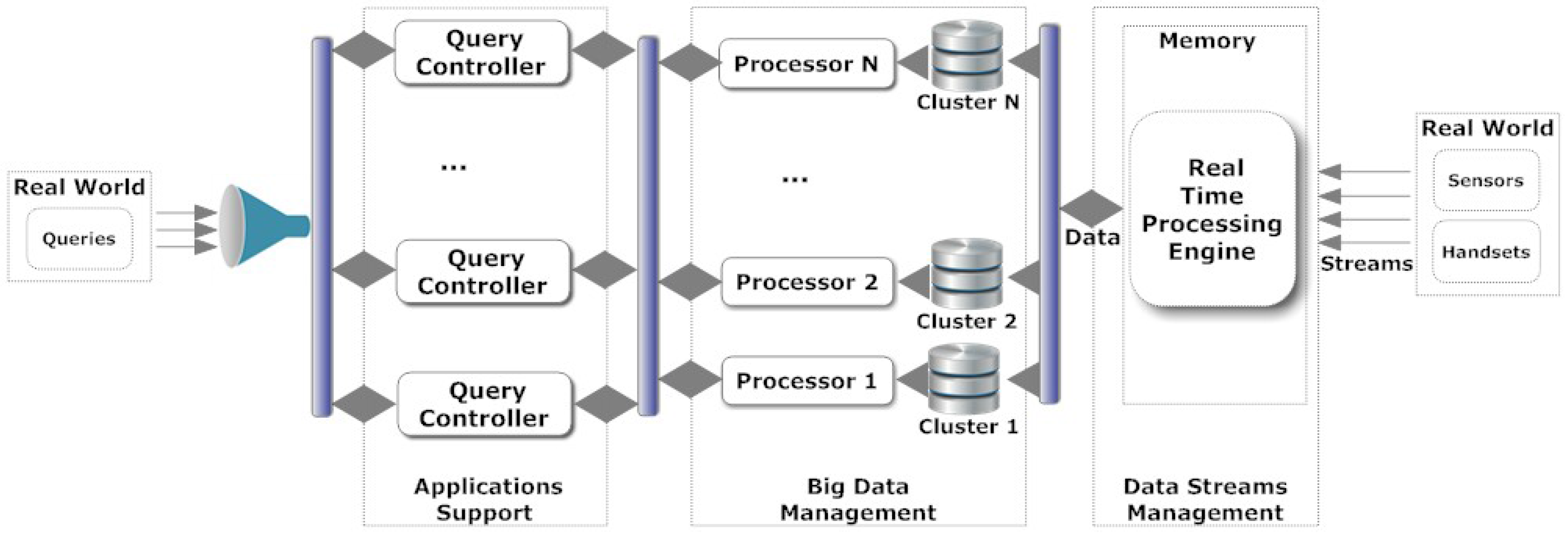
Figure 2.
The proposed Q-tables (the ‘assign’ column depicts the ‘assignment’ action).

Figure 3.
The training time.
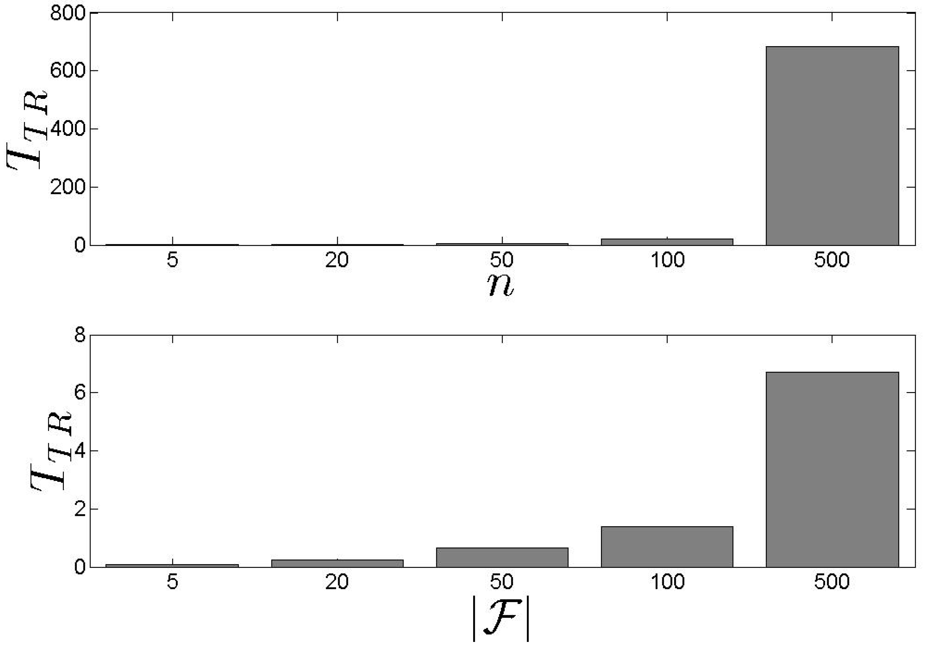
Figure 4.
The initial set of clusters creation time.
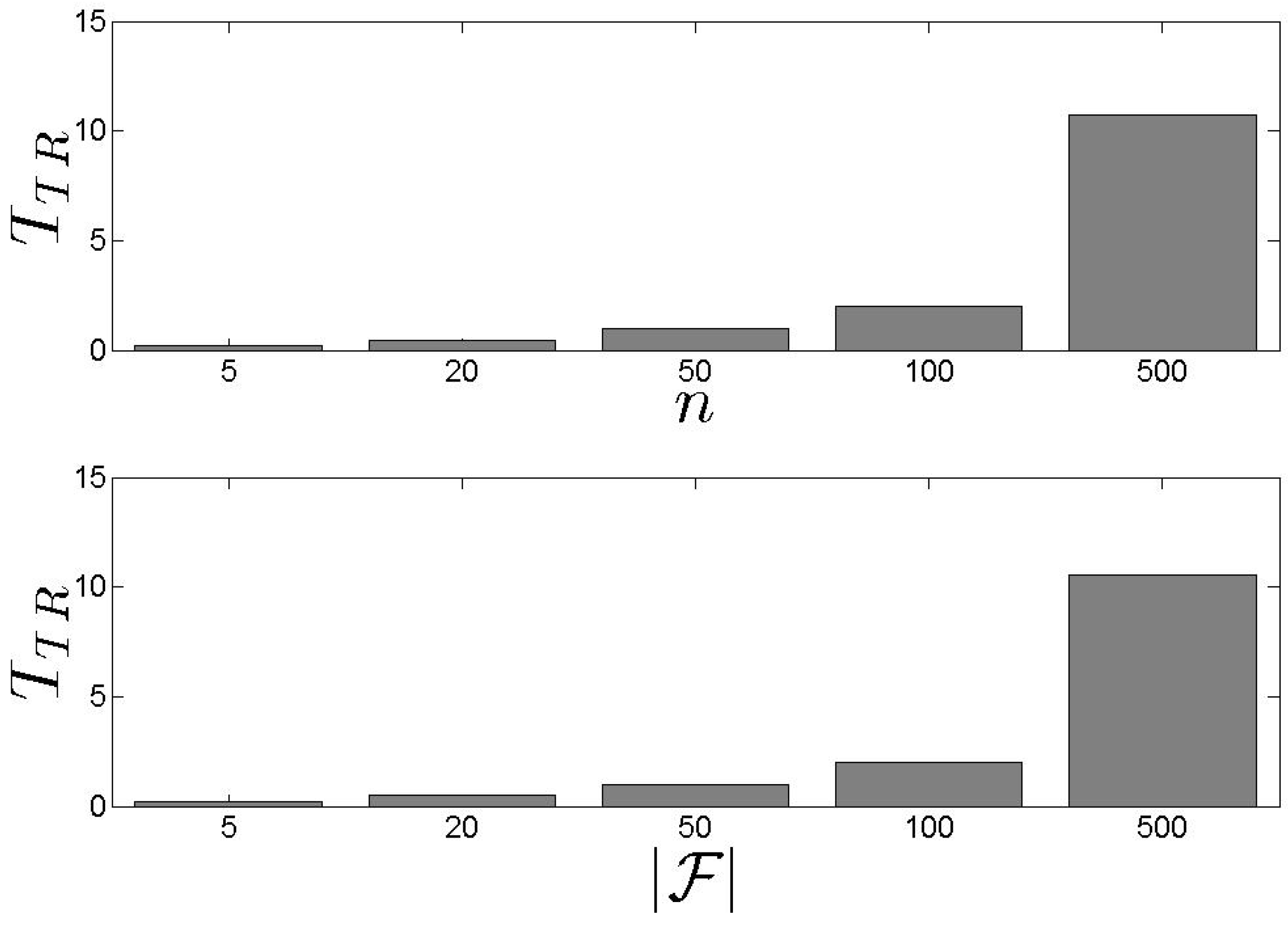
Figure 5.
Our results for the throughput of the and the .
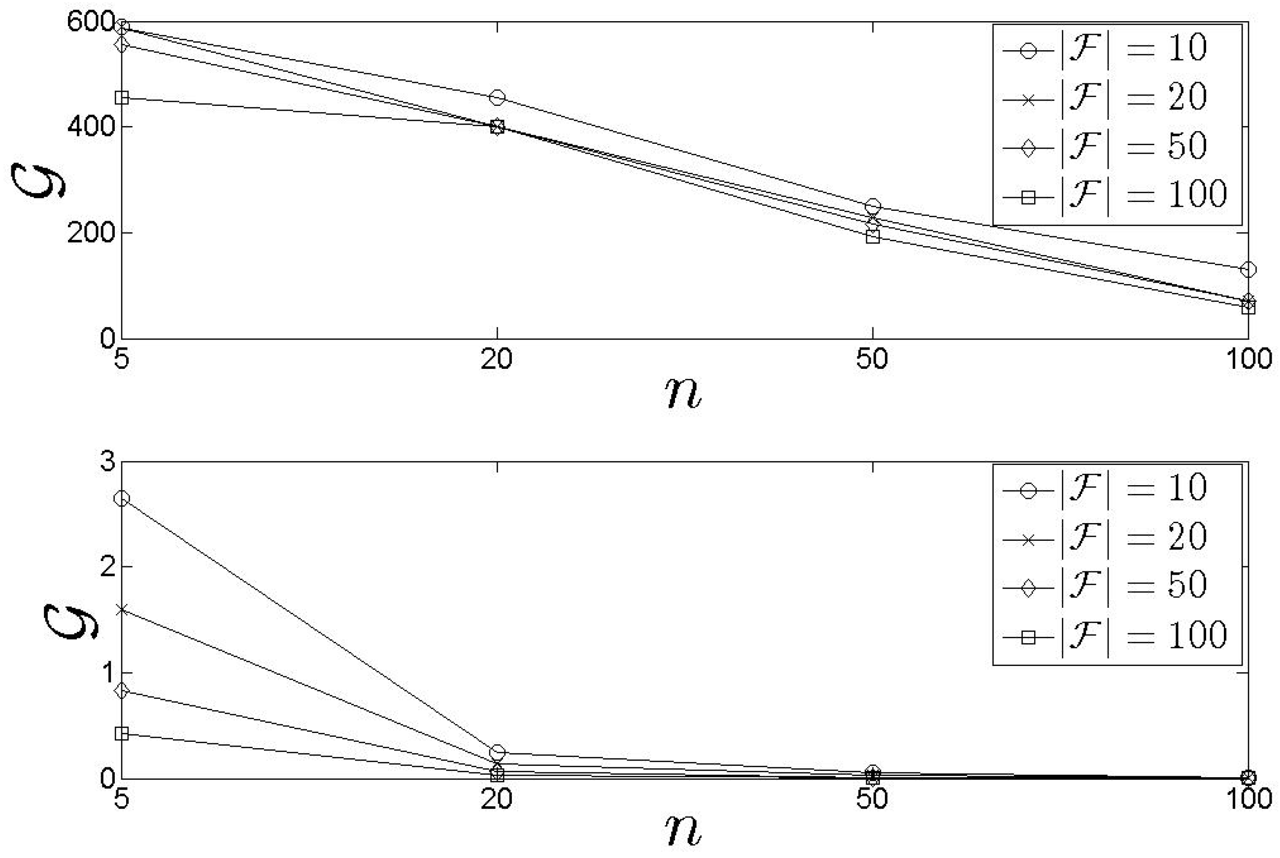
Figure 6.
and results for the metric ().
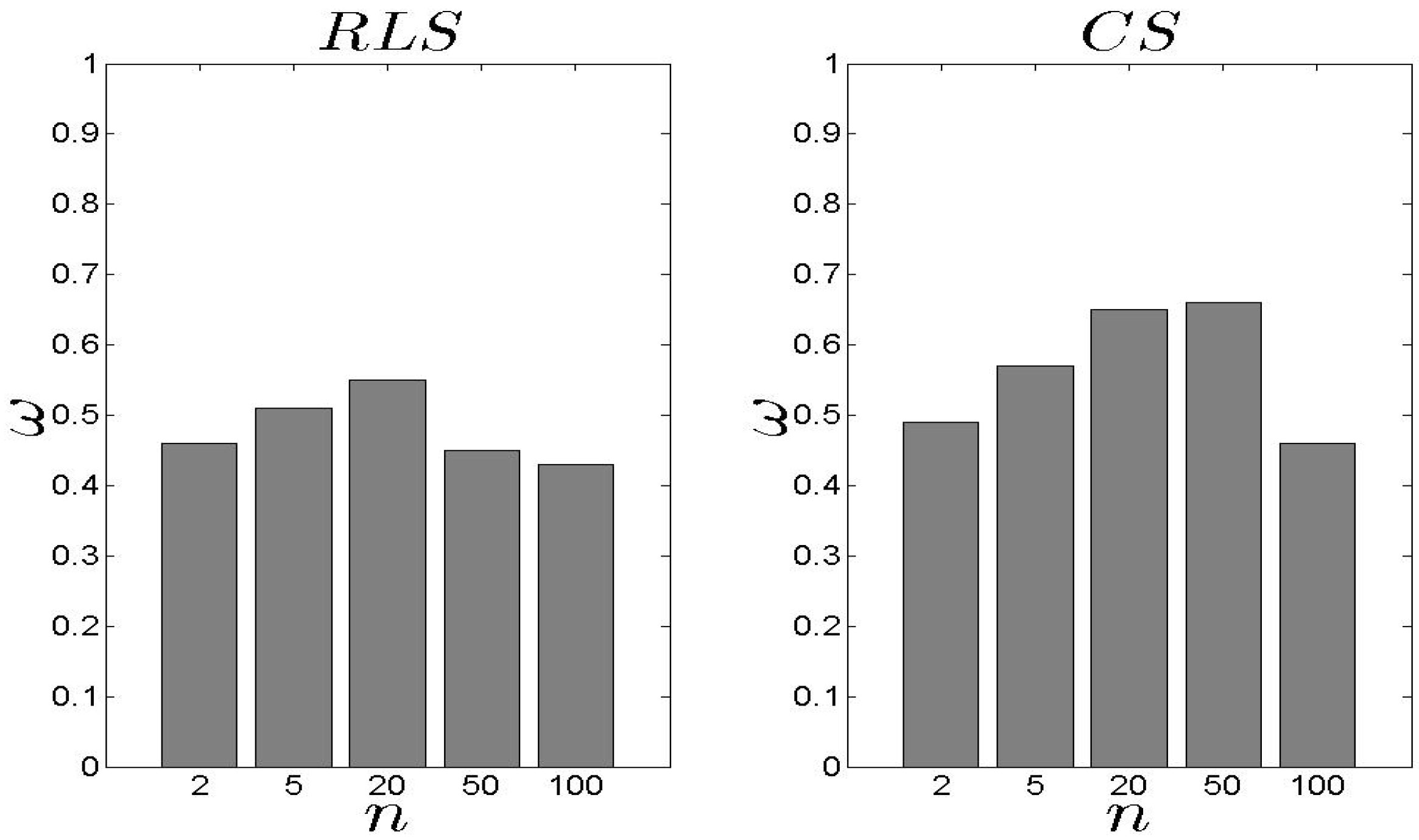
Figure 7.
and results for the metric ().

Figure 8.
and results for the metric ().
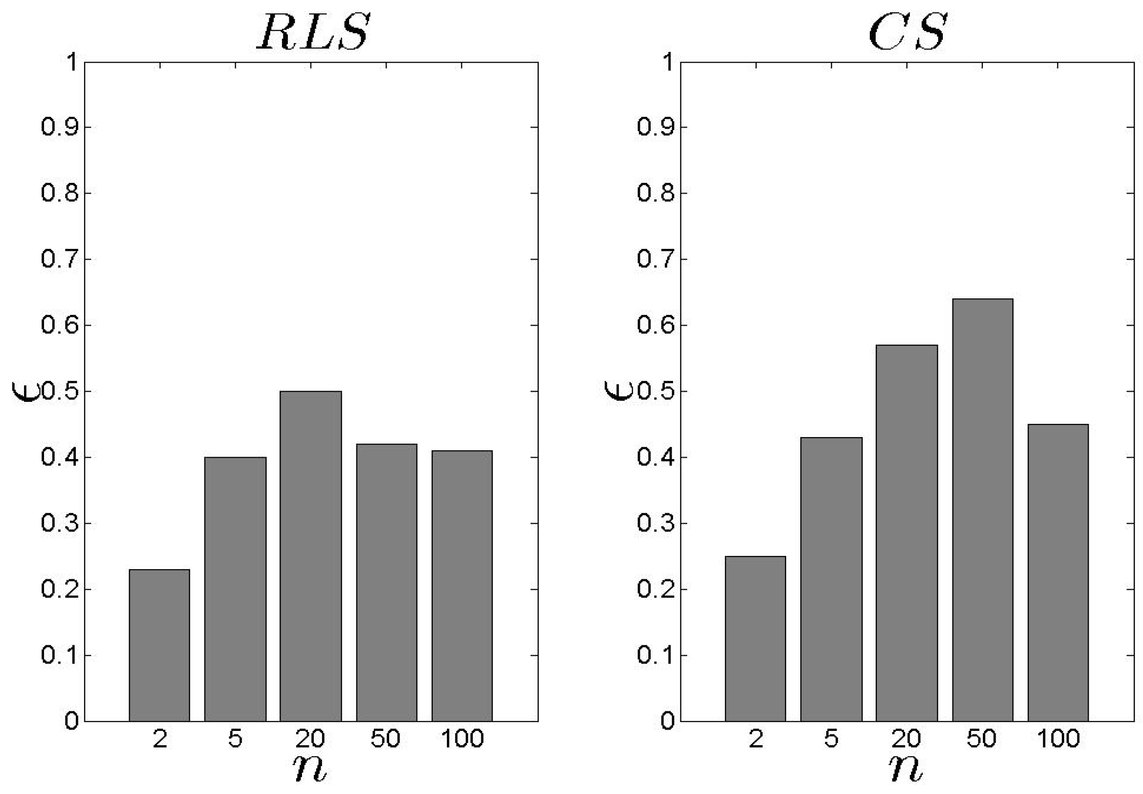
Figure 9.
and results for the metric ().

Figure 10.
and results for the metric.
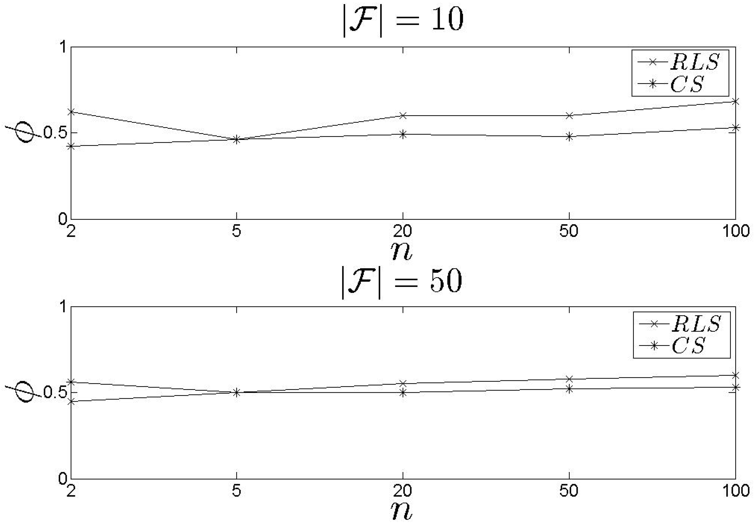
Figure 11.
and results for the metric ().
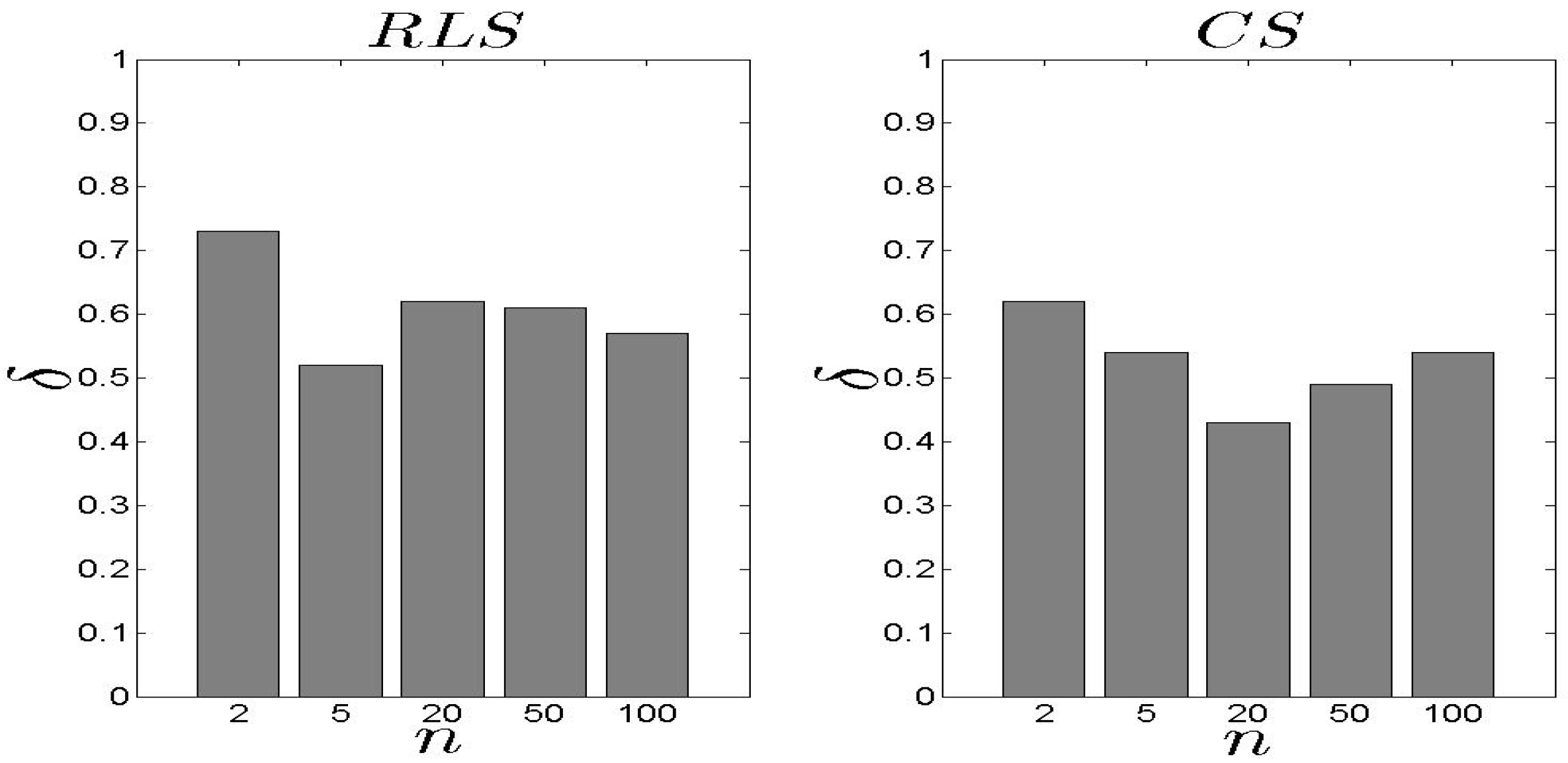
Figure 12.
and results for the metric ().

Figure 13.
and results for the metric ().

Figure 14.
and results for the metric ().

Figure 15.
results for the .
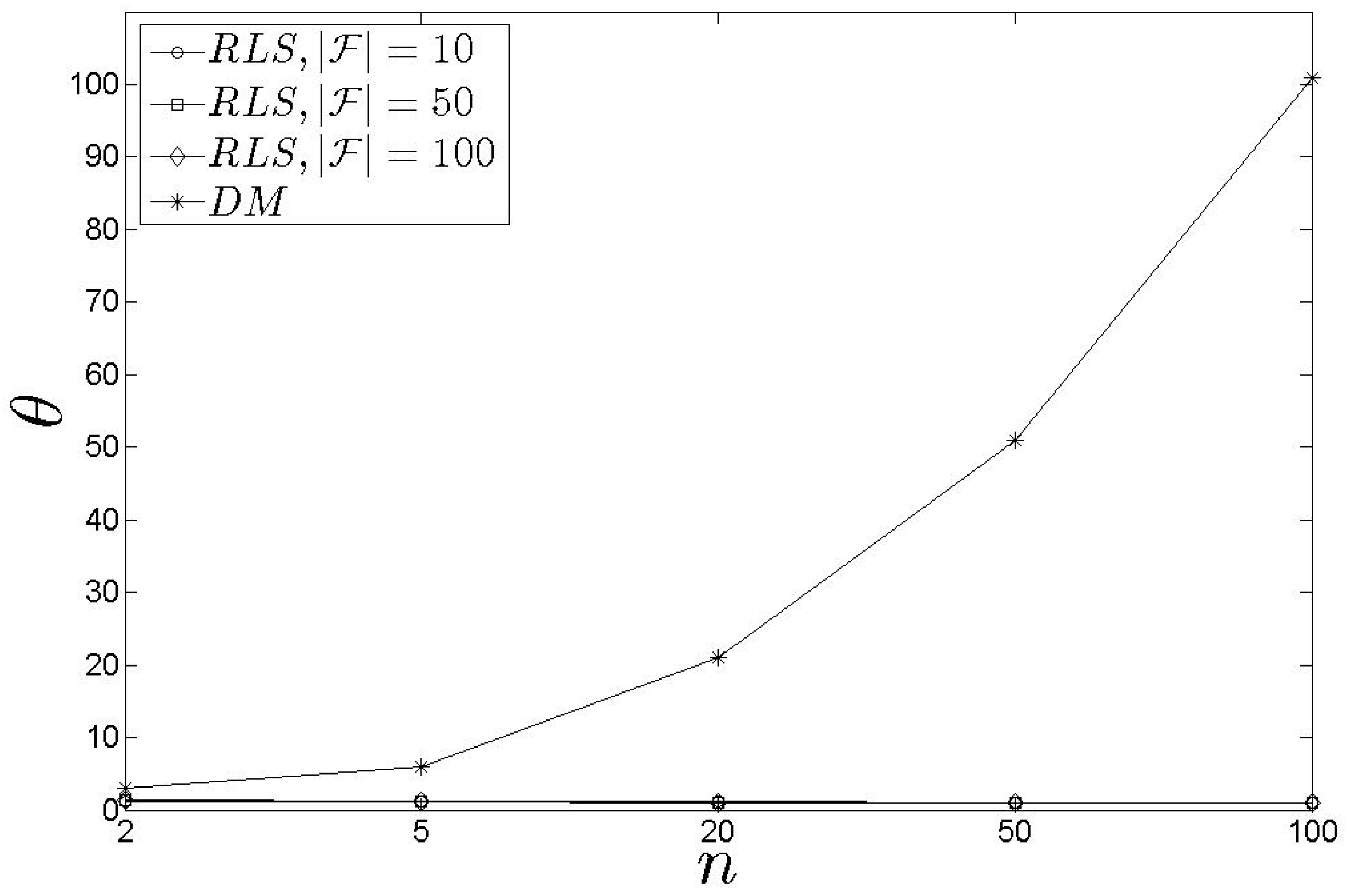
Figure 16.
Comparison results with the .


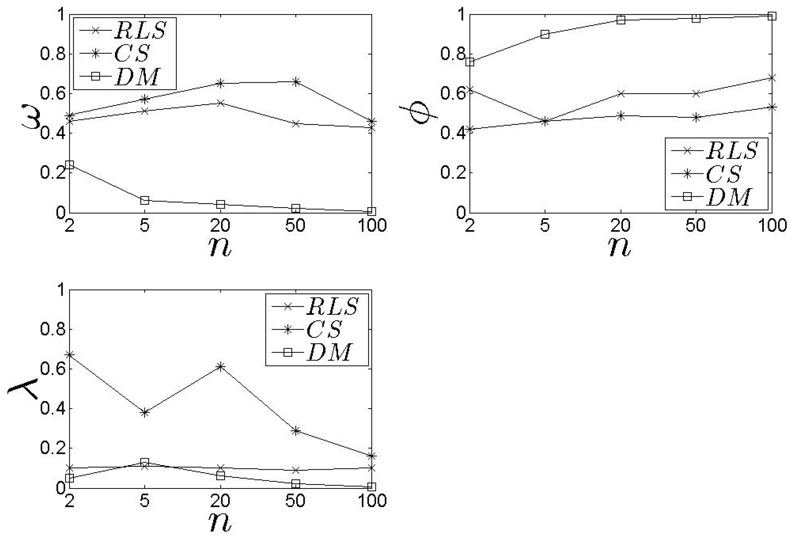
Table 1.
Predictors List.
| Predictor | Attributes | Short Description |
|---|---|---|
| Cycle | Window size | It returns the same data in a specific window |
| Single Exponential | Smoothing factor | It consists of a weighted average of past values |
| Double Exponential | Smoothing factor | It uses a simple linear regression equation |
| Seasonal Naive | Seasonal period | Each forecast is equal to the last observed value from the same season in the past |
| Drift | Time window | Time window |
| Extrapolation | - | It estimates the value of a variable on the basis of its relation with another variable |
| Additive Holt Winters | Level, Slope, Season | It deals with time series containing both trend and seasonal variations |
| Multiplicative Holt Winters | Level, Slope, Season | It deals with time series containing both trend and seasonal variations |
| Geometric Moving Average | Window size | It smooths past data by geometrically averaging over a specified period and projects forward in time |
| Moving Average | Window size | It smooths past data by arithmetically averaging over a specified period and projects forward in time |
| Parabolic Moving Average | Trend value | It is a weighted moving average with weights that form a parabolic shape |
| Triangular Moving Average | Window size | It is a weighted moving average with weights that form a triangular shape |
| Neural Network | Network nodes | It uses a neural network for estimating future values |
| Linear | Coefficients | It uses the Levinson-Durbin algorithm for linear prediction |
| Linear Regression | Coefficients | It fits the time series to a straight line and projects forward in time |
| Polynomial | Coefficients | It fits a polynomial equation to the data and projects forward in time |
| Rounded Average | Window size | It returns the rounded average of past values defined in a specific window |
Table 2.
results for different n.
| n | ||
|---|---|---|
| 2 | 0.54 | 1.19 |
| 5 | 0.57 | 1.87 |
| 20 | 0.54 | 5.69 |
| 50 | 0.50 | 13.12 |
| 100 | 0.49 | 25.52 |
© 2017 by the authors. Licensee MDPI, Basel, Switzerland. This article is an open access article distributed under the terms and conditions of the Creative Commons Attribution (CC BY) license (http://creativecommons.org/licenses/by/4.0/).
Share and Cite
MDPI and ACS Style
Kolomvatsos, K.; Anagnostopoulos, C. Reinforcement Learning for Predictive Analytics in Smart Cities. Informatics 2017, 4, 16. https://doi.org/10.3390/informatics4030016
AMA Style
Kolomvatsos K, Anagnostopoulos C. Reinforcement Learning for Predictive Analytics in Smart Cities. Informatics. 2017; 4(3):16. https://doi.org/10.3390/informatics4030016
Chicago/Turabian StyleKolomvatsos, Kostas, and Christos Anagnostopoulos. 2017. "Reinforcement Learning for Predictive Analytics in Smart Cities" Informatics 4, no. 3: 16. https://doi.org/10.3390/informatics4030016
Note that from the first issue of 2016, this journal uses article numbers instead of page numbers. See further details here.