
Visual Analysis of Stochastic Trajectory Ensembles in Organic Solar Cell Design


1
Department of Science and Technology, Linköping University, 60174 Norrköping, Sweden
2
Department of Physics, Chemistry and Biology, Linköping University, 58183 Linköping, Sweden
3
Institute for Media Informatics, Ulm University, 89081 Ulm, Germany
*
Author to whom correspondence should be addressed.
Informatics 2017, 4(3), 25; https://doi.org/10.3390/informatics4030025
Submission received: 31 May 2017
/
Revised: 24 July 2017
/
Accepted: 26 July 2017
/
Published: 1 August 2017
(This article belongs to the Special Issue Scalable Interactive Visualization)
Abstract
:We present a visualization system for analyzing stochastic particle trajectory ensembles, resulting from Kinetic Monte-Carlo simulations on charge transport in organic solar cells. The system supports the analysis of such trajectories in relation to complex material morphologies. It supports the inspection of individual trajectories or the entire ensemble on different levels of abstraction. Characteristic measures quantify the efficiency of the charge transport. Hence, our system led to better understanding of ensemble trajectories by: (i) Capturing individual trajectory behavior and providing an ensemble overview; (ii) Enabling exploration through linked interaction between 3D representations and plots of characteristics measures; (iii) Discovering potential traps in the material morphology; (iv) Studying preferential paths. The visualization system became a central part of the research process. As such, it continuously develops further along with the development of new hypothesis and questions from the application. Findings derived from the first visualizations, e.g., new efficiency measures, became new features of the system. Most of these features arose from discussions combining the data-perspective view from visualization with the physical background knowledge of the underlying processes. While our system has been built for a specific application, the concepts translate to data sets for other stochastic particle simulations.
1. Introduction
In the quest to tap renewable energies, the development of organic solar cells plays an important role as they can be manufactured in high throughput at low prices. Additionally, the flexibility of these cells offers many benefits compared to conventional solar cells. Unfortunately, despite organic solar cells are already used in a few commercial products, their comparably low efficiency currently forbids a wide-spread use.
The efficiency of an organic solar cell is directly related to its molecular structure, which is usually formed by two aggregations of molecules (donor and acceptor) that are sandwiched between two electrodes. When photon absorption occurs it leads to the formation of excitons (electron-hole pairs), which are transported to the electrodes, whereby the donor transports the holes and the acceptor the electrons. The time to reach the electrodes is determined by the molecular structure of the donor as well as the acceptor, and inversely proportional to the efficiency of the cell. Thus, to improve the efficiency of organic solar cells, it is mandatory that the underlying physical principles regarding charge transport are better understood, and that an optimal molecular structure can be predicted. Kinetic Monte-Carlo simulation is a tool frequently used in this context to better understand the behavior of charge transport, by establishing a relation between the material structure and a solar cell’s properties [1,2,3]. By simulating a multitude of charges traversing the sandwiched region large charge-transport trajectory ensembles are obtained. Understanding of these charge-transport trajectory ensembles and their connection to the molecular structure is key to be able to design more efficient organic solar cells [4].
In this paper, we propose an analysis system composed of a set of linked spatial visualizations together with plots of structure-aware trajectory measures. The structure of the data is similar to trajectories resulting from tracking of movement data and thus the exploration concepts are similar. However, an efficient exploration system requires a configuration targeted specifically toward the needs of the application. Accordingly, novel concepts were also needed for the proposed system. A central requirement for the charge trajectory analysis is relating the stochastic microscopic data to macroscopic efficiency measures. To achieve this, the concept of charge-flow lines has been introduced. They mimic the macro-level behavior of charges resulting in typical flow descriptors as flow direction and velocity. The morphology of the solar cell under investigation serves as context.
Thus, within this paper, we make the following contributions:
- We propose a set of linked visualization techniques that enable the investigation of dense charge-transport trajectory ensembles by exploiting trajectory abstraction and relating trajectories to a solar cell’s morphology.
- We propose novel geometric measures to analyze the efficiency of individual trajectories and trajectory ensembles based on the concept of charge flow lines.
- We discuss how these components are integrated into a single visualization framework, which supports domain experts when visually analyzing organic solar cell simulations.
The remainder of the paper is structured as follows. In the next section, we briefly describe the application background and describe the visual analysis tasks we have identified as being essential when exploring the data at hand. In Section 2, we summarize the most important recent work that inspired the development of our framework. Section 3 starts with an overview of the proposed visualization framework, and introduces the applied visualizations and the novel efficiency measures. In Section 4, we describe the technical details. To demonstrate the effectiveness of our framework we apply it to simulation results with different levels of complexity, with respect to the underlying physical model, and discuss the findings made in Section 5. Finally, the paper concludes in Section 6.
1.1. Application Task Characterization
In the following, we will describe how the visual analysis tasks have been developed since they play a central role for the configuration of the system. The overall goal has been to gain a deeper understanding of the process of charge transport based on the simulation results. However, as it is often the case when scientists look at their data for the first time, there were no clear questions to start from and the analysis has been driven by the question: ‘Let’s see what we will find.’ More specific tasks have then been gradually identified within a close collaboration between visualization experts and theoretical physicists who perform the simulations. The visualization system has been developing continuously by new hypotheses that have been developed during the visual exploration, see Figure 1.
The first task, which we call the Overall Efficiency (OE), aims to give an overview of the data in its most original form. This means displaying the trajectory ensemble as a whole and allow simple interaction to inspire new questions to guide the further development of the system. This matches the visual-information seeking mantra: Overview first, zoom and filter, then details-on-demand. During the configuration of the system the visualization tasks have been shifting more and more from a microscopic to a macroscopic view. This reflects a generalization of the questions starting from the modeling perspective on the quantum mechanical level to questions related to large-scale properties as the efficiency of the probe. The macroscopic view has to a large extend been new to the physicists and triggered many new ideas for the design of the simulation. Understanding of the interaction between the scales is what finally paves the way for the further development of the technology.
The pertinent questions that arose during the development of the system can be summarized as follows. Morphology Efficiency (ME): Understand the general distribution of charges and the impact of the morphology geometry on the distribution and the transport properties. Thereby the individual trajectories have not been considered as very interesting. Charge Interaction (CI): A complementary question is the role of charge interactions for the charge transport. These questions involve the inspection of individual charge pair trajectories but also the morphology and especially the material interface as context. For these questions the fully detailed trajectories hide the trends of the transport and there is a demand for abstraction and macroscopic views and measures to quantify the efficiency. Simulation Evaluation (SE): Orthogonal to the questions targeting toward understanding the underlying physics, is the evaluation of the performance of the simulation and its parameter settings. Therefore it is important to easily inspect the plausibility of the results and identify outliers. For this purpose almost all proposed visualizations are useful whereby simple geometric settings are of advantage.
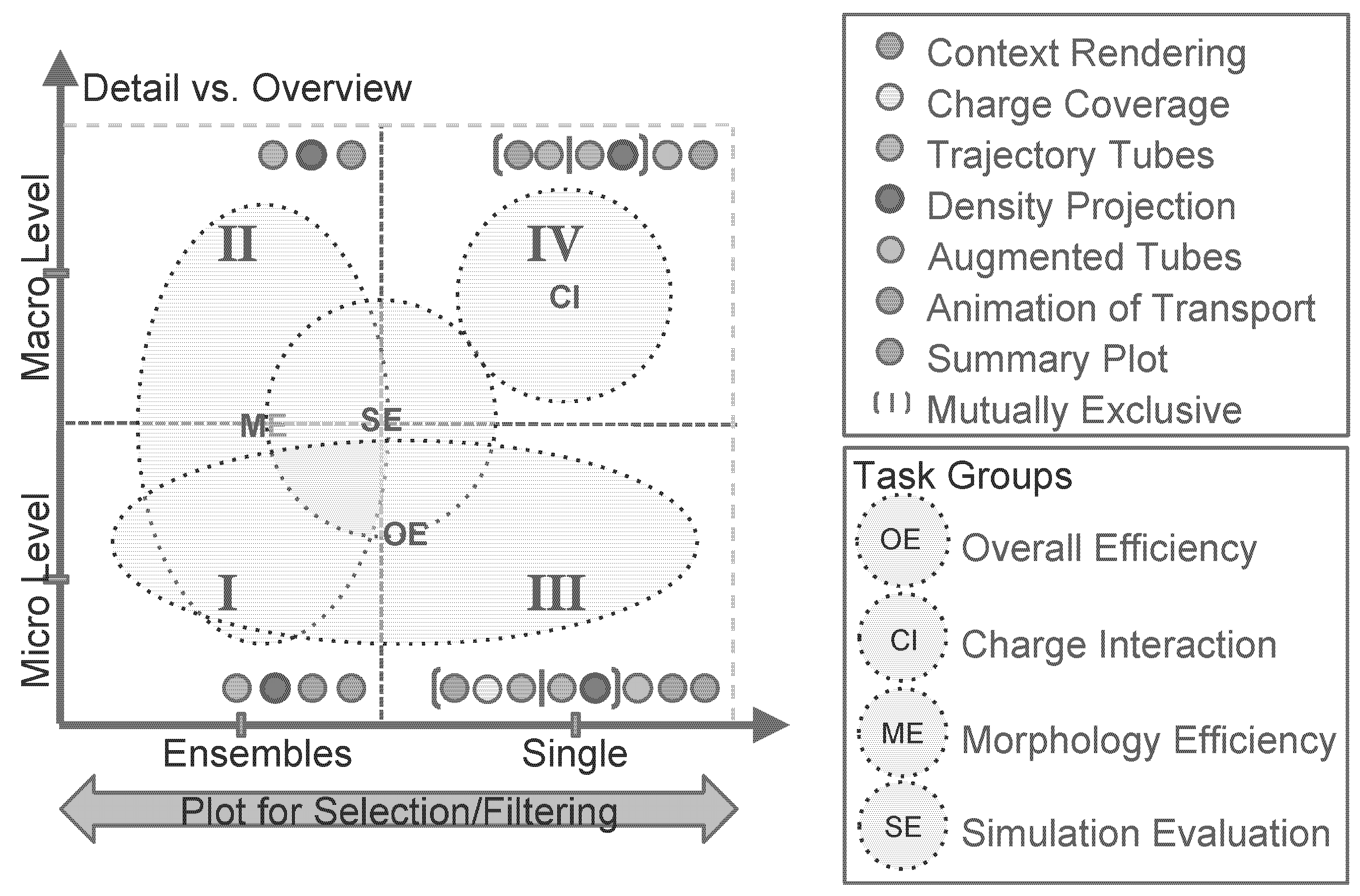
The derived tasks suggest the employment of a two-dimensional visualization parameter space. One dimension pertains to the level of detail and abstraction ranging from a micro-level to a macro-level view. The second dimension relates to the number of trajectories that are investigated ranging from the entire ensemble to single trajectory analysis. We divide the parameter space into four quadrants as illustrated in Figure 2. The proposed methods and derived task are placed into this space to provide an overview.
1.2. Organic Solar Cell Design
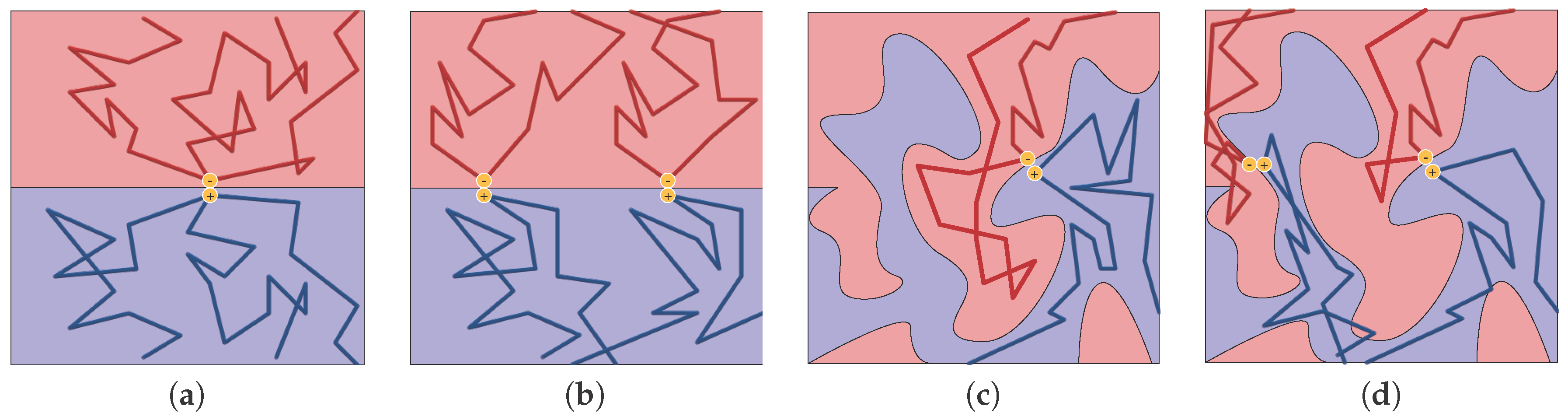
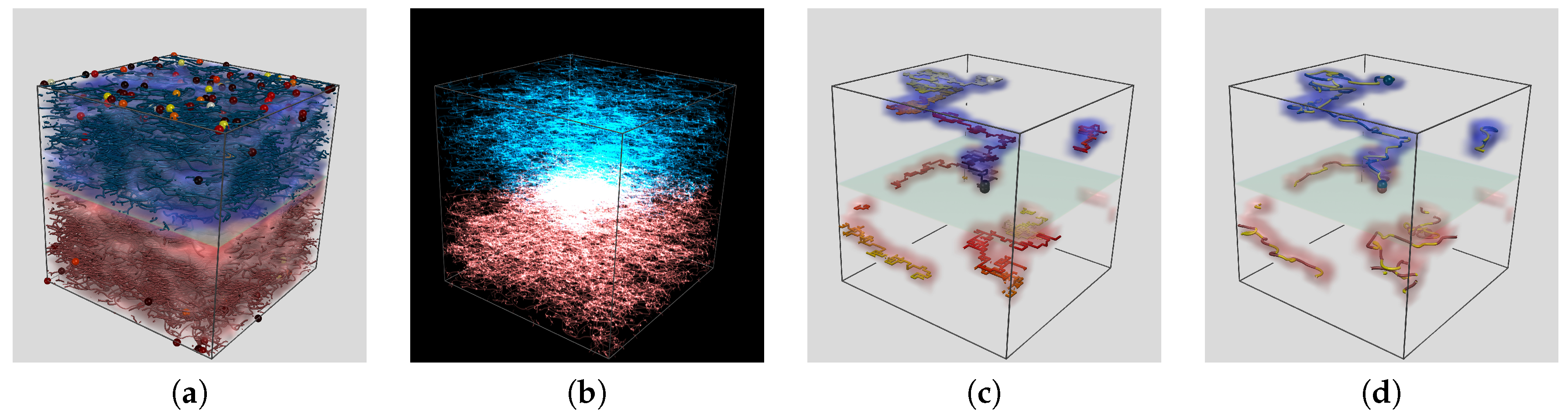
To understand the benefits of the proposed visual analysis framework, some information regarding the application background needs to be provided first. The efficiency of an organic solar cell is determined by the efficiency of the different steps from photon absorption to charge collection. As these are directly related to the structure, different structures for such cells have been investigated. The simplest consisting of a layer of an organic semiconductor between two electrodes. However, the performance of a cell can be improved by having two layers of organic materials: the donor and the acceptor [5] (see Figure 3a,b). In a working solar cell, photons are absorbed generating excitons, which then diffuse toward the interface as illustrated in Figure 3a,b and form a charge transfer (CT) state. The CT states then split into free electrons and holes that can be collected at the electrodes. While Figure 3a shows this case for a single exciton, Figure 3b illustrates the existence of two excitons. After the charge carriers are freed, they may still move back to the interface and recombine. Here, two types of recombination can occur: geminate and nongeminate. Geminate recombination is when two charge carriers resulting from the absorption of the same photon recombine. Nongeminate recombination occurs when two free charge carriers originating from different photons recombine with each other at the interface.
The morphology of the donor-acceptor interface in an organic solar cell has a large impact on the efficiency of the solar cell. Excitons can only diffuse 10 nm before decaying, so the donor and acceptor should be sufficiently mixed, as otherwise the excitons could not reach the interface before decaying. An example of a more complex morphology is illustrated in Figure 3c,d. However, once separated, the charge carriers need pathways to their respective electrodes. If, for example, an electron is in an acceptor domain that is completely surrounded by the donor, there is no path for the electron to travel to the electrode. Consequently, it is important to establish a morphology-efficiency relationship and determine for instance how the domain size and tortuosity influence the different processes, such as transport of the exciton, dissociation of the CT, and free charge carriers transport.
Because of the amorphous nature of the material and the probabilistic nature of the competitive processes at play in a solar cell, stochastic methods such as the Monte-Carlo approach are applied. In our setup, a kinetic Monte-Carlo code is used where the hoping rates are calculated based on the Marcus Equation [6] using a multi-scale approach [1,2]. Based on the simulation parameters, these simulations result in a variety of data, whereby we focus on the analysis of the trajectory ensembles in combination with the morphology data. The trajectories are realizations of possible charge propagations based on a physically accurate transition probability from molecule to molecule. Each trajectory represents a sequence of discrete positions associated with one specific molecule and an associated dwell time. Along a trajectory, charges jump back and forth and may be trapped in some regions due to multiple physical fields interacting with the charges. To get a representative description of the charge movement an ensemble of trajectory-pairs representing one CT is computed, whereby each trajectory of the ensemble is represented as a discrete series of molecule identifiers and the dwell time at the respective molecule. All trajectories of one ensemble start at the same position. Thus, trajectories usually do not represent shortest paths within the constraints of the morphology. The morphology of the material consists of two materials, the acceptor and the donor material. It is represented as a volumetric data set generated by an ergodic process, whereby binary values (donor = 1, acceptor = 0) are used to mask the voxels.
1.3. Some Details about the Data
The data is a result of a kinetic Monte-Carlo simulation consisting of two parts: the geometry information of the material morphology and the charge trajectories. The morphology is represented as a volumetric data set, where each voxel encodes the material type, acceptor or donor, as a binary value. The interface between the acceptor and the donor is presented by an isosurface for the isovalue of 0.5. The morphology serves as a container for the donor and acceptor molecules. In the setting of our simulations the molecules are placed on a regular grid thus corresponding to the morphology data set. The morphology is the most important context information for the trajectories. For all visualizations we use a color schema assigning blue to donor material and electron trajectories and red to acceptor material and whole trajectories, if not stated differently.
The charges are always attached to one molecule. The transport is modeled as a probabilistic process for charges hopping from one molecule to the next according to a quantum-mechanical transition probability. Each charge trajectory thus consists of a series of molecule-IDs augmented with information such as dwell time and the type of the charge (electron or hole). Since the trajectories represent a stochastic process they are not smooth. Often, charges hop frequently back and forth between neighboring molecules. Each simulation run represents one possible path of a charge pair, a hole and an electron, which influence each other. The initial configuration for all trajectories of the entire ensemble are the same. This concerns the initial position of the charge pair and the morphology. The simulation assumes periodic boundary conditions, meaning a charge leaving the volume on one side will enter it again on the opposite side.
2. Related Work
In the following, we summarize previous work that is mostly related to our work. Thereby we focus on (i) previous visualization systems developed for similar applications in solar cell design; (ii) visualization and analysis of trajectory and movement data; (iii) rendering methods for lines; (iv) related ensemble visualization; and (v) efficiency measures for stochastic particle movements.
(i) Related applications. The work most closely related to our visualization system is the work by Aboulhassan et al. [7]. They are concerned with the same application, the design of efficient organic solar cells and the task of exploring the efficiency of the charge transport. However, from a data perspective of the system it differs a lot from our work. Their system has been designed to explore structural characteristics of the morphology [8] while we focus on the explicit charge trajectories resulting from a Monte-Carlo simulation. Therefore, they propose a topological approach for the simplification of the morphology and distill a geometric backbone as simplification of the complex structure. Geometric bottlenecks for the charge transport are extracted from the backbone. Previously, the same authors developed a system for visual design of solar cell crystal structures [9]. To analyze these structures, the user can exploit semantic rules to define clusters of atoms with certain geometric properties. While the idea of knowledge-assisted exploration plays also an important role in our system, we focus on the exploration of the charge trajectories, which is a complementary task. Accordingly, we also do not discuss molecular visualization techniques, which would be required to explore the actual solar cell structure. Instead we refer to the recent state-of-the-art report by Kozlikova et al. [10], which covers most relevant techniques.
(ii) Analysis and visualization of trajectory and movement data. The analysis of trajectories is also a central task when dealing with motion tracking and movement data. Even though the applications are very different the data structure has some similarities. In both cases one deals with a large numbers of trajectories that are not smooth and allow crossings. Some challenges related to overplotting and clutter are similar. In an overview article about visual analytics of movement by Andrienko et al. [11,12] they classify the related work into four categories: Looking at trajectories, looking inside trajectories, bird’s-eye view on movement, and investigating movement in context. These categories are also related to our parametrization of the visualization space. However, there are also some essential differences. The charge trajectories are three-dimensional and thus cannot easily be embedded in two-dimensional map representations. There are no interactions between trajectories for different ensemble members and the movements of the charges has a stochastic character. Therefore, filtering and efficiency measures are in general not transferable.
(iii) Trajectory visualization. Our application deals with a vast amount of trajectories, which need to be explored within the morphological context. Therefore, effective visualization of dense line sets is important. Several approaches to tackle similar problems have been developed for flow data or in medical context for fiber visualization. A typical approach is focus and context technique that enables an occlusion-free view into the trajectories, such that the trajectory under investigation becomes visible. An early work using this concept for flow data visualization has been presented by Doleisch et al. [13]. Flow features in focus are emphasized whereas the rest of the data are shown as context. Gasteiger et al. [14] applied the idea for the visualization of blood flow data. The focus and context technique employed by our system has been inspired by these approaches, whereby the morphology of the solar cell provides the context. Besides an occlusion-free view, an unambiguous perception of the visualized trajectories is important. There exist many approaches for rendering of large sets of lines. Much effort has been put on improving the spatial perception of occluding and overlapping lines. One way to approach this problem is to use illuminated lines [15,16]. Applying tubes or other geometries for the line rendering allows for more advanced methods. Techniques have been proposed reaching from the use of halos, ambient occlusion and the use of smart transparency. Such methods have been combined for enhanced molecular visualization by Tarini et al. [17]. Techniques exploiting halos have been frequently applied for the rendering of fibers in the medical field [18,19,20,21]. Schröder et al. [22] enhance illuminated lines with ambient occlusion in combination with transparency and halos to achieve a good depth perception and thus improve the visual quality of dense integral line rendering. A further trend to enhance the expressiveness of renderings in the use of illustrative visualizations. An overview of related methods for flow visualization is presented by Brambilla et al. [23]. To convey information about local flow properties, Everts et al. [24] proposed to augment flow lines with strips. We adopted this method for the visualization of properties of the charge flow lines derived from the charge trajectories. Another way to deal with large set of lines is to use filtering methods using line predicates as proposed by Salzbrunn et al. [25].
Most of the above described methods are however not appropriate for the rendering of the original charge trajectories, which are stochastic in their nature and non-smooth. Charges are hopping back and forth frequently between same spots, whereby the individual hops are not of particular interest in contrast to the dwell time in certain regions. A method that is well suited to highlight regions where the charges preferably stay is the method of trajectory density projection for vector field visualization by Kuhn et al. [26]. This is an efficient approach for large amount of trajectories reducing the clutter and occlusion due to the number of curves exploiting capabilities of modern graphics hardware. The rendering results in images giving a good impression of the distribution and density of trajectories. To combine the rendering of our charge flow lines, which are explicit geometry with the density distribution volume data, we intended to adopt an approach by Lindholm et al. [27]. They propose a hybrid data visualization method based on a depth complexity histogram analysis. But for sake of simplicity we used approach by Henning [28] since we assumed the geometry of charge flow lines to be opaque.
(iv) Ensemble visualization. An important aspect of our application is the interplay between the ensemble of trajectories and the individual lines. Ensembles receive more and more attention in the field of visualization, which is especially challenging for vector data. Typical visualizations are a combination of spaghetti plots of lines with appropriate statistical plots. Examples from the field of weather forecast can be found in Sanyal et al. [29] or Wilson et al. [30]. Ferstl et al. [31] use a clustering of flow lines, which are then visualized using variability plots representing the distribution of each cluster. These variability plots have some similarity with our charge coverage visualization.
(v) Efficiency measures. For the analysis and characterization of complex trajectories diverse measures have been used. Bos et al. [32] introduced angular statistics to reflect the multi-scale dynamics of pathlines in turbulent flows. Their measure reflects the multi-scale dynamics of high-Reynolds number turbulence. Savage et al. [33] also use an angular measure to characterize the diffusion process of charges in context with the analysis of perfluorosulfonic acid membranes. They investigate the caging effect of water and the hydrophobic moieties on the motion of the excess proton. In their method, they consider the relative angle between the vectors of motion for two successive time intervals as a probe of the directional changes in the diffusion process. Burov et al. [34] analyze random walks considering the distribution of relative angles of motion between successive time intervals, which provides information about the underlying stochastic processes. Some of these measures are related to our transport efficiency measures; however, none fits our setting of charges moving within a discrete regular grid within a constrained geometry. Instead of analyzing angles on multiple scales, we consider the effective distance and velocity of the charges on multiple scales.
3. Trajectory Exploration Framework
To explore the data on all levels, we have designed a framework that combines multiple spatial views on different levels of abstraction with statistical plots. It enables selection of trajectories and a detailed inspection of those. It allows to explore the data starting with overview representations and drilling down to more detailed visualizations in both dimensions of the visualization parameter space: moving from ensembles to individual trajectories and from macro-level to micro-level views. Thereby, we exploit typical visualization concepts like multiple linked views, focus and context visualization and brushing and linking. Figure 4 shows an example screen shot of the proposed system. In the following we first describe the various spatial views Section 3.1 then we discus the set of plots and efficiency measures that have been introduced Section 3.2.
3.1. Spatial Views
For each quadrant of the visualization parameter space a set of spatial visualizations are provided, which are described briefly in the following. For all visualization one can chose between the original simulation volume or an expended volume respecting the periodic boundary conditions unfolding the trajectories, see Figure 5. To encode the temporal aspect of the data we use color or animation, steered by a time slider.
3.1.1. Quadrant I: Ensemble Visualization, Microscopic View
The visualizations provide the most direct view on the data, Figure 6c. Thereby the morphology represents the context and the entire ensemble is in focus. Even though the individual trajectories are not of interest, the trajectories are still plotted in their original form as solid lines with all details. An example is shown in Figure 5. This visualization suffers heavily from over-plotting and is mostly useful for debugging purposes. However, it allows the domain scientists to quickly grasp the transport activity of charges in a material and has been used frequently to get a first impression of the data and its correctness.
3.1.2. Quadrant II: Ensemble Visualization, Macroscopic View
From an macroscopic ensemble perspective, Figure 6a, often the trajectory details are not of much interest. In that case, it makes sense to switch to the macroscopic view. It only displays the density distribution and the coverage of all trajectories highlighting regions in the morphology where the charges dwell for a longer time. We provide thereby two options for trajectory rendering. The charge coverage volume focuses on displaying coverage by generating a volume representing the frequency of charge-visits for each location in the morphology, see Figure 10a. The trajectory density projection [26] accumulates transparent slightly smoothed trajectories in one image, see Figure 10b for a simple morphology and Figure 13c for a complex morphology. These renderings allow conclusions about the transport efficiency with respect to the morphology and the detection of possible traps.
3.1.3. Quadrant III and IV: Inspection of Individual Trajectories
When exploring a few selected trajectories, Figure 6b,d–h, the context is not only given by the morphology but can also include the entire ensemble. Moving from microscopic to macroscopic view can be considered as a smooth transition from the stochastic data to smooth lines. For all these visualizations we consider pairs of trajectories consisting of an electron and a hole. They can influence each other and should always be inspected jointly. Thereby the lowest level of abstraction is the direct representation of the trajectory data. It renders every charge jump from one molecule to the next. The resulting trajectories are aligned to the grid structure defined by the molecular structure, Figure 6d. On the other end of the scale one can either look at the charge coverage volume for the selected trajectory or a gradual simplification of the trajectory. Due to the strong stochastic character of the trajectories, simple Gaussian smoothing does not give the desired results. Therefore, we introduced flow lines capturing the trend of the large-scale movement. Flow lines are motivated by the transition from the Brownian motion of water molecules to a continuous flow description. The detailed construction of the lines will be described in Section 4.1.
For any simplification level one can chose between tube and ribbon rendering. For a higher level of abstractions the lines can also be augmented with derived attributes emphasizing the large scale flow properties like velocity and flow direction, which are not well defined for the original data. For their visualization color, textures and arrows are used. The effective velocity is encoded using stripe patterns displaying equal time intervals.
3.2. Statistical Plots and Efficiency Measures
The plots represent characteristic measures relevant for the assessment of the simulation data. They serve as a basis for the interaction and filtering of the data and are linked to the spatial renderings. Thereby trajectories of interest can be selected in the plots as well as in the spatial representations. As for the spatial plots we always consider a pair of electron and hole. To be able to distinguish the different charge types we assign positive values to electron-related measures and negative values to hole-related measures. Trajectory plots associate characteristic measures to the trajectories. The x-axis represents the straightened charge trajectories (hop-id or time), e.g., Figure 11a–d. Parallel coordinates relate different efficiency measures for the individual trajectories, Figure 11e. Morphology Composition plots allow to investigate the material composition in the neighborhood of a selected charge position, Figure 7.
Essential for the effectiveness of the statistical plots are the attributes that are displayed. Therefore, much emphasis has been put on the design of expressive measures for the efficiency of the charge transport. The derivation of the measures described below, has already been a result of the first visual exploration of the data in close collaboration with the physicists. The goal of the measures is to get a qualitative impression of the efficiency of the charge transport from creation to collection at the electrodes. The measures can be related to (i) individual trajectories, (ii) charge pairs, or (iii) the morphology. All measures can be explored on an ensemble or single trajectory basis.
- (i)
- Trajectory-based measuresThese measures have the purpose to equip the macro-level charge flow lines with measures that are commonly related to flow. A central measure is the effective velocity, which describes the macro-level charge velocity. The measures can be adapted to the chosen level of detail via a scale parameter r. The unit for r is intermolecular distance.
- Escape time . The escape time of a charge from molecule with respect to scale r is defined as the time the charge needs to leave the r-neighborhood of the molecule, see Figure 8c. It is high in regions where the charge is trapped for a longer time. The dwell time at a molecule corresponds to the escape time for .
- Effective velocity . The effective velocity is directly related to the escape time. Low velocity hints at low efficiency in the charge transport, this can be due to traps in the morphology or a strong inter charge interaction.
- Effective distance traveled —The effective distance is the Euclidean distance of the current charge position to the start position as function of time. This measure is related to the escape time but allows a stronger focus on the geometry of the trajectory.
- Tortuosity —Tortuosity sets the actual path length of the trajectory in relation to the effective distance traveled .
- (ii)
- Charge pair related measuresThe morphology of the material is not the only critical aspect for the efficiency of the charge transport. There is also a strong interaction between individual charge pairs influencing their transport. If charge pairs come very close to each other, this comprises the risk of recombination, which means that the charge is lost for the entire process.
- Pair distance —This distance measure keeps track of the Euclidean distance of a hole and an electron created in one CT state. In the optimal case this would be a monotonously increasing function of time.
- Minimal distance to charge of other kind —In the case of multiple CT states a recombination is not only possible with the own ‘partner’ (geminate recombination) but with all charges of the complementary type (nongeminate recombination). In this way it is a generalization of .
- Minimal distance to charge of same kind —Charges of the same type interact with each other and can thus reduce the effective transport. This measure gives an overview over the distribution of the charges within the material. Charges of the same type interact with each other and can thus reduce the effective transport. This measure gives an overview over the distribution of the charges within the material.
- (iii)
- Morphology related measuresThe morphology is a critical parameter for the design of the solar cells. While a large interfacing surface is advantageous for the creation of CT states, a complex morphology can crate traps for the charge transport.
- Distance to interface —This distance is the shortest distance of molecule to the material interface. It is computed once for each morphology. As distance metric we use a Manhattan metric following the molecular grid structure. Thus the distance roughly corresponds to the minimal number of charge transitions necessary to reach the interface. Since recombination of charges only happens at the material interface it is favorable that the charges keep a certain distance to the interface.
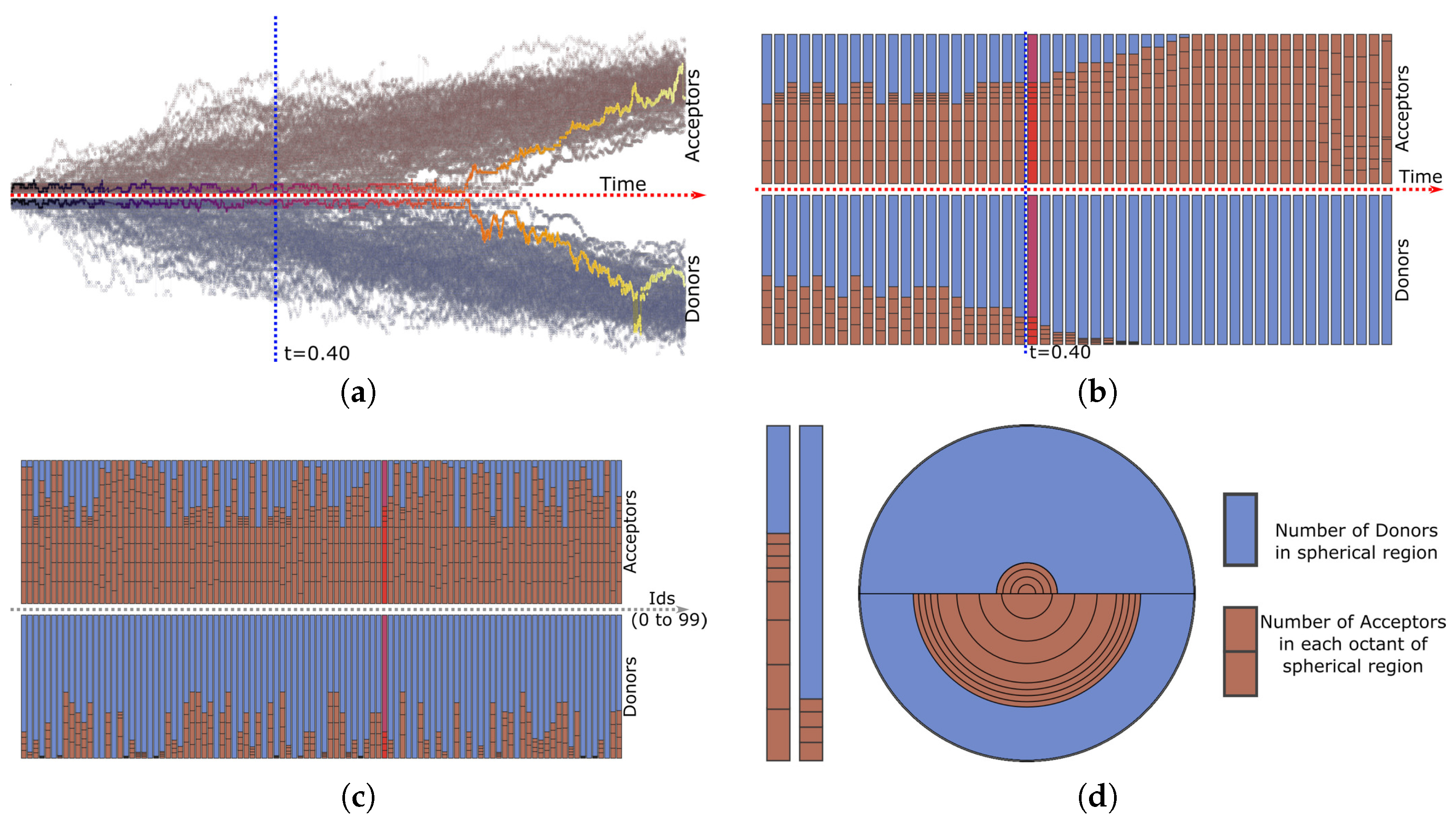
- Morphology Composition plots—Through these plots the morphology composition (acceptor-donor ratio) can be investigated. It displays the acceptor-donor material ratio in the neighborhood surrounding a charge. For a single trajectory, the ratio is plotted for the entire transportation (Figure 7b). For ensembles, the morphology ratio at a specific time (Figure 7c) is plotted. The acceptor-donor ratio is computed for a spherical region. The spherical region is divided into eight octants illustrating the distribution in each octant. (Figure 7d).
4. Technical Details
In this section we summarize few technical details that are necessary for the implementation and rendering of flow lines.
4.1. Charge Flow Lines
As the trajectories are the result from a Monte-Carlo simulation of charges jumping between discrete locations they are bound to the grid of the molecular structure and are very tortuous at the same time (Figure 8a). To get a better impression of the trend of the trajectories we propose two different approaches for simplification: smoothing and charge flow lines.
Trajectory smoothing corresponds to a simple Gaussian smoothing taking only every n-th sampling position into account. The parameter n can be interactively adjusted, which is especially useful for the density projection rendering where we typically used a value of n = 4. Gaussian smoothing mostly improves the rendering results; however, it is not suitable to highlight macroscopic flow properties as effective charge velocity. Since the complexity of the trajectories changes considerably along the trajectory no global smoothing factor would lead to satisfactory results. Therefore we introduced the notion of flow lines to convey the trend of the movement of the charge. It is defined on various abstraction levels, expressed by a scale factor r. The generation of flow lines can be interpreted in analogy to the transition of the stochastic Brownian movement of molecules in a flow and the macro-level description as a smooth line with direction and velocity. To generate a flow line the trajectory is sub-sampled ignoring all transitions within a sphere of radius r, compare Figure 8b. The time the charge needs to escape the sphere defines its effective velocity on the abstraction level r. The radius r is defined in units of the molecular grid cell size. As described above, the charge flow lines are rendered as solid lines with arrows encoding the direction of movement. An example of different abstraction levels for one charge trajectory is shown in Figure 8. The local trajectory complexity is reflected by its tortuosity and is also an important indicator for local transport efficiency.
4.2. Ribbon Computation
We use ribbons mostly for the representation of trends in the movement of charges based on the concept of flow lines introduced above. The ribbon computation uses a moving frame of reference for the flow lines, see Figure 9e,f. This frame is determined by its tangent, its normal, and its binormal. The normalized tangent is approximated by the direction of the line segment. To obtain a stable normal computation, especially in region with low curvature, we introduce a weighted normal propagation
The weight is a measure for the stability of the normal. If it is close to 1 the previous normal has no influence, if it is close to zero ( is parallel to ) the previous normal is propagated. For placement of ribbon arrows we compute the curvature of the line and the high curvature segments are filtered out. Figure 9d,g,h, shows ribbon arrow segments that are placed using this approach.
5. Use Cases
The visualization system became an integral part in the research project for organic solar cell design and the understanding of charge transport in complex materials. Typical for basic research projects is that questions and new tasks are developing at the same pace as getting new insights and answers. For that reason, there are only few tasks that are frequently performed in exactly the same way. In the following we describe two scenarios, in which the system has be used and insights that have been derived. We put the tasks into the context of the task classification introduced in Section 1.1. We start with a simple setting focusing on the simulation evaluation (Task SE). To illustrate scenarios where the exploration is driven by a domain specific task with the goal of gaining new insight (Tasks OE, CI and ME) we consider a more complex setting using a complex morphology. For all visualizations we use color-coding of red for acceptor and blue for donor material, the interface between the two regions is rendered as a green transparent surface. The observations discussed in the following sections summarize the reasoning of our partners when exploring the data with our system.
5.1. Scenario 1—Simple Planar Interface One CT
This scenario refers to a simple planar interface between the donor and acceptor material of the solar cell considering one CT, which corresponds to one charge pair. The ensemble consists of 100 different realizations of charge paths, whereby all paths start at the same location and diffuse toward the electrodes, which are placed on the top and the bottom of the volume. This configuration is of special interest for the evaluation of the simulation correctness and parameter setting (Task SE) since for this simple case there are clear expectations toward the results.
Derived insights: The distribution of the ensembles is expected to be approximately uniform, which is confirmed by the trajectory coverage visualization for the entire ensemble in Figure 10a. The slight variations that are visible in the charge coverage volume are due to the stochastic sampling of the space of possible charge trajectories using 100 realizations.
The spheres on the top and bottom of the volume highlight the locations where the charges reach the electrodes, their color displays the time-to-electrode for the respective trajectory. The ensemble density projection shown in Figure 10b allows a more detailed view into the volume highlighting preferred locations. As to expect for this setting, the region exhibiting the highest density is the area of the joint starting point in the center of the image. Figure 10c,d show one selected trajectory with a long time-to-electrode value. Even though the time the charge needed to get to the electrode is relatively high it is continuously moving in the expected direction and the path and its effective velocity appear plausible. The progression plots shown in Figure 11 confirm these findings. After a short time of strong interaction with the partner charge the charges continuously move toward the electrodes. All plots show that the two charges have a very symmetric behavior. Inspecting selected trajectory. plot (b) and (c) express the long interaction time of the charges until they finally separate and then quickly diffuse toward the electrodes. Plot (a) shows that during the interaction time the charges even visit their initial position again. A qualitatively similar behavior can also be observed for other charge pairs whereas the specific point in time where the charges start traveling independently strongly varies. This can also be seen in the parallel coordinates plot where it seems that there is no clear correlation between the time and the effective distance traveled. However, there is a strong correlation between the distance to the interface and the distance to the other charge. Plot (d) showing the escape time, expresses a general decrease of the escape time over time, which is confirmed in the parallel coordinate plot. The higher escape times at the beginning of the trajectory are a hint that the charge interaction traps the charges and slows their movement down due to attracting forces. All these measures that are represented in the parallel coordinates plot can be used to filter out and explore trajectories of interest. In summary, all the plots and spatial renderings support the reasoning and understanding of the most significant physical effects controlling the efficiency of the transport.
For some of the simulation runs a surprising observation has been made in the visualizations of the charge coverage volume. There, charges exhibited a tendency to stick close to the interface for a very long time never reaching the electrodes, Figure 12a. A closer inspection of the trajectories in temporal animations and in flow line representations made clear that this is due to the strong interaction between the charge pairs. The strength of this effect only became aware to the physicist through these visualizations. A similar observation was later also made for the complex morphology, Figure 12b. While it was possible to find an explanation of this effect, it was not expected in this clarity and it motivated us to make changes in the parameter setting for the external field that drives the diffusion process of the charges. This observation also lead to the introduction of a new efficiency measure the ‘distance between charge pairs’ shown in Figure 11b. These plots show the time it takes for charge pairs to separate and finally take off toward the electrodes. An inspection of the parallel coordinates plot of the efficiency measures also strengthened this explanation and makes it clear that the effect is not related to a long escape time.
5.2. Scenario 2—Complex Interface Exploration
The second scenario is an exploration of the results of an ensemble simulation for a complex morphology considering one respective two CTs, which is one respective two charge pairs moving from the start point to the electrodes. The three tasks OE, CI and ME have been driving this exploration. We started the exploration with overview representations, Figure 13, for the entire ensemble and use one exemplary plot where some trajectories showed a behavior that draws interest. In the second part we explore these trajectories in more detail, Figure 14.
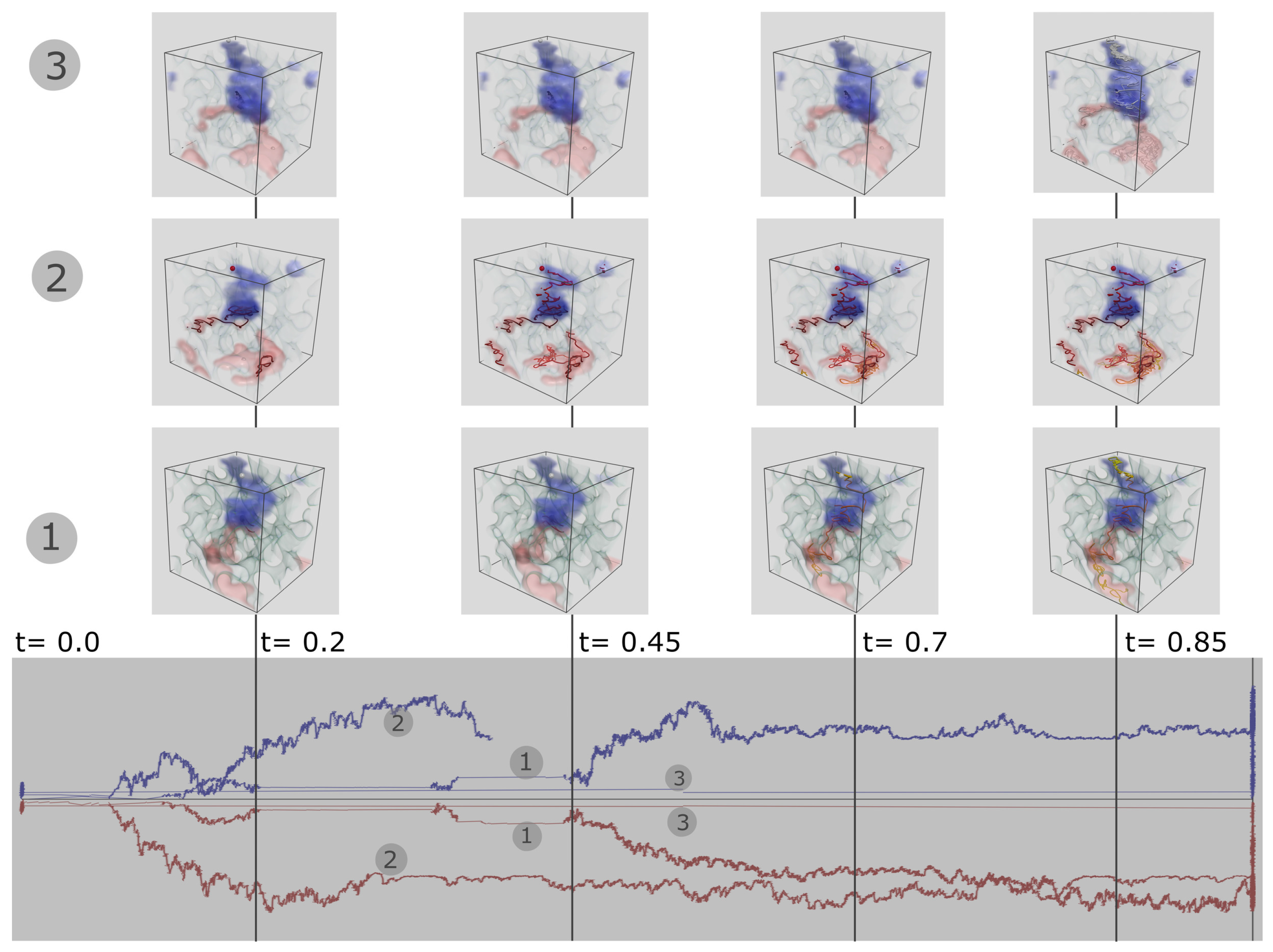
The collection of the entire ensemble within the morphology is displayed in Figure 13. The columns give an impression of the temporal evolution of the charge transport. The rows provide different ensemble visualizations for the four time steps. The top row (a) shows the charge coverage volume within the morphological context and the highlighted endpoints of the trajectories colored by time-to-electrode. The second row (b) shows only the trajectories without the morphology. The third row (c) uses the density projection plot highlighting preferred regions for the trajectories. The last row (d) shows the linked plots of the progression of the distance to the interface. They are composed of a summary plot overlying the evolution of the entire ensemble (left) individual trajectories that can be used for selection (right). A vertical line in these plots specifies the selected time step for the respective column.
Derived insights. The volume coverage visualization in row (a) shows that the charge paths of the ensemble are widely distributed within the volume. However, it also can be seen that they preferably move in the right direction, donor (blue) charges upward and acceptors (red) charges downward toward the respective electrode not being dragged in the wrong direction by the morphology, row (b). The locations where the charges reach the electrode do not have any preferred area on the electrode shown by the distribution of the spheres on the electrodes. Also the time-to-electrode value seems not to correlate to the location where the charge reaches the electrode. The density plots in row (c) highlight regions where the charges stay for a longer time. Besides the starting location and the electrodes there are some ’chambers’ in the morphology, which show a higher density. The plots give insight into the charge interaction (Task CI) showing the trend that most trajectories initially stay close to the start position for some time until the charges escape the attraction of the partner charge and finally start moving toward the electrodes.
The patterns visible in the other plots are very different as compared to the simple morphology. While the dwell time in the simple morphology decays rapidly, the distribution of the dwell time for the complex topology stays the same for the entire time. The charges interact much longer with each other staying closely together and following similar paths. The escape time shows much higher peaks. A high escape time is a measure for a trapping of the charges. Symmetric behavior to the donor and acceptor hints at trapping due to CT effects and charge interaction. In the cases where we only see high values for one charge, the trapping must be related to other morphology effects.
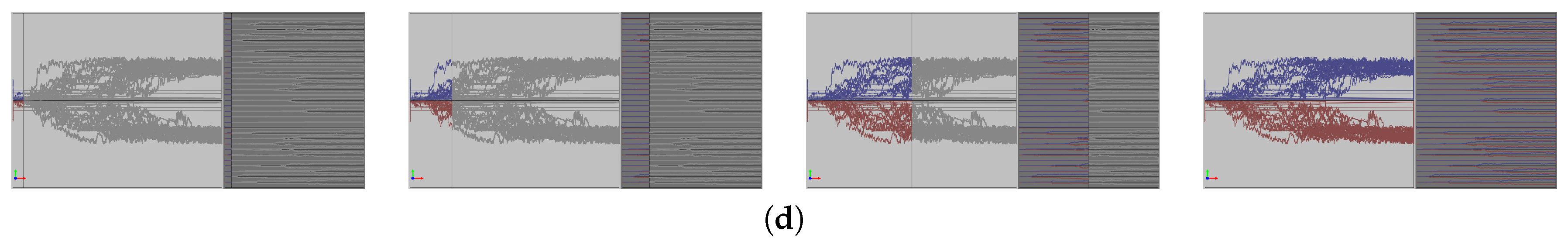
Individual trajectory inspection—The second part of the exploration was focused on details of the data as required for task CI and ME. Three selected trajectories with peculiar behavior were detected in the effective-distance-travelled plot, Figure 14. The trajectories are analyzed using one of the trajectory plots. In Figure 14, time of charge transport is mapped to the x-axis and the distance from the start point of charge transport to the y-axis. Acceptor and donor can be distinguished in all images by the color red and blue respectively. The three rows refer to the three selected trajectories.
Derived insights. The plot gives hint about outlier trajectories and the CT can be examined within this context. Trajectory (1) in Figure 14 has expected charge transport, in contrast to trajectory (2) and (3). In trajectory (2), one of the charge pairs stopped propagation much earlier than the other. In trajectory (3), there was some transport in the beginning of the simulation and the propagation stopped before they started propagating again in the end. This indicates a long pause during the CT.
6. Conclusions
In summary, we have presented a framework for the exploration of ensembles of charge trajectories in the context of material morphology. Our partners have considered all individual visualizations and plots as useful; however, the special merit of the system lies in the combination of the plots and visualizations. This allows us to focus on individual trajectories as well as the ensemble as distribution. Thereby, the distribution gives insight into the overall efficiency of the solar cell design. The exploration of individual trajectories is useful to analyze the effect of the morphology on the charge transport. Many aspects of the data were accessible for the first time to our partners. Most importantly, all the plots and renderings have supported the reasoning about the characteristics of the charge transport in organic solar cells and the performance of the simulation itself. It inspired many vivid discussions, which help to understand the most significant physical effects controlling the efficiency of the transport. In several cases, the findings influenced the next simulation run and the adjustment of the simulation parameters. The discussions also inspired many new ideas for follow-up work. The efficiency measures that are now part of the system have been developed on the basis of the first versions of the visualization system and thus prove the usefulness of the visualization system. In the future will integrate other physical fields involved in the simulation into the exploration framework as context information. It is further planned to extend the system to less regular molecular structures and more diffuse interfaces, which is ongoing work for our collaboration partners. Many of the concepts derived for this application can also be of use for other applications that are concerned with ensembles of stochastic trajectories.
Acknowledgments
This work was supported through grants from the Swedish e-Science Research Centre (SeRC) and has been developed in the Inviwo framework (www.inviwo.org).
Author Contributions
All authors have been contributing essential in the development of the concepts of the visualization system and writing the paper. Sathish Kottravel is mainly responsible for the implementation of the visualisation system. Mathieu Linares and Riccardo Volpi are the Physicists that performed the simulation of the charge transport and are responsible for the data generation.
Conflicts of Interest
The authors declare no conflict of interest.
References
- Jakobsson, M.; Linares, M.; Stafström, S. Monte Carlo simulations of charge transport in organic systems with true off-diagonal disorder. J. Chem. Phys. 2012, 137, 114901. [Google Scholar] [CrossRef] [PubMed]
- Volpi, R.; Stafström, S.; Linares, M. A consistent Monte Carlo simulation in disordered PPV. J. Chem. Phys. 2015, 142, 094503. [Google Scholar] [CrossRef] [PubMed]
- Volpi, R.; Kottravel, S.; Norby, M.S.; Stafström, S.; Linares, M. Effect of Polarization on the Mobility of C60: A Kinetic Monte Carlo Study. J. Chem. Theory Comput. 2016, 12, 812–814. [Google Scholar] [CrossRef] [PubMed]
- Volpi, R.; Linares, M. Organic Solar Cells. In Specialist Periodic Reports—Chemical Modelling; RSC: London, UK, 2016; Volume 13. [Google Scholar]
- Tang, C.W. Two-layer organic photovoltaic cell. Appl. Phys. Lett. 1986, 48, 183–185. [Google Scholar] [CrossRef]
- Marcus, R.A. On the Theory of Oxidation, Reduction, Reactions Involving Electron Transfer. J. Chem. Phys. 1956, 24, 966. [Google Scholar] [CrossRef]
- Aboulhassan, A.; Baum, D.; Wodo, O.; Ganapathysubramanian, B.; Amassian, A.; Hadwiger, M. A Novel Framework for Visual Detection and Exploration of Performance Bottlenecks in Organic Photovoltaic Solar Cell Materials. Comput. Graph. Forum 2015, 34, 401–410. [Google Scholar] [CrossRef]
- Wodo, O.; Tirthapura, S.; Chaudhary, S.; Ganapathysubramanian, B. A graph-based formulation for computational characterization of bulk heterojunction morphology. Org. Electron. 2012, 13, 1105–1113. [Google Scholar] [CrossRef]
- Aboulhassan, A.; Li, R.; Knox, C.; Amassian, A.; Hadwiger, M. CrystalExplorer: An Interactive Knowledge-Assisted System for Visual Design of Solar Cell Crystal Structures. EuroVisShort 2012. [Google Scholar] [CrossRef]
- Kozlikova, B.; Krone, M.; Lindow, N.; Falk, M.; Baaden, M.; Baum, D.; Viola, I.; Parulek, J.; Hege, H.C. Visualization of Biomolecular Structures: State of the Art. EuroVisSTAR2015 2015. [Google Scholar] [CrossRef]
- Andrienko, N.; Andrienko, G. Visual analytics of movement: An overview of methods, tools and procedures. Inf. Vis. 2012, 12, 3–24. [Google Scholar] [CrossRef]
- Andrienko, G.; Andrienko, N.; Bak, P.; Keim, D.; Wrobel, S. Visual Analytics of Movement; Springer: Berlin, Germany, 2013. [Google Scholar]
- Doleisch, H.; Hauser, H.; Gasser, M.; Kosara, R. Interactive Focus + Context Analysis of Large, Time-Dependent Flow Simulation Data. Simulation 2006, 82, 851–865. [Google Scholar] [CrossRef]
- Gasteiger, R.; Neugebauer, M.; Beuing, O.; Preim, B. The FLOWLENS: A focus-and-context visualization approach for exploration of blood flow in cerebral aneurysms. IEEE Trans. Vis. Comput. Graph. 2011, 17, 2183–2192. [Google Scholar] [CrossRef] [PubMed]
- Zöckler, M.; Stalling, D.; Hege, H.C. Interactive visualization of 3d-vector fields using illuminated stream lines. In Proceedings of the IEEE Conference on Visualization (Vis ’96), San Francisco, CA, USA, 27 October–1 November 1996; pp. 107–114. [Google Scholar]
- Schussman, G.; Ma, K.L. Anisotropic Volume Rendering for Extremely Dense, Thin Line Data. In Proceedings of the IEEE Conference on Visualization ’04, Austin, TX, USA, 10–15 October 2004; pp. 107–114. [Google Scholar]
- Tarini, M.; Cignoni, P.; Montani, C. Ambient Occlusion and Edge Cueing to Enhance Real Time Molecular Visualization. IEEE Trans. Vis. Comput. Graph. 2006, 12. [Google Scholar] [CrossRef] [PubMed]
- Everts, M.H.; Bekker, H.; Roerdink, J.; Isenberg, T. Depth-Dependent Halos: Illustrative Rendering of Dense Line Data. IEEE Trans. Vis. Comput. Graph. 2009, 15, 1299–1306. [Google Scholar] [CrossRef] [PubMed]
- Eichelbaum, S.; Hlawitschka, M.; Scheuermann, G. LineAO—Improved Three-Dimensional Line Rendering. IEEE Trans. Vis. Comput. Graph. 2013, 19, 433–445. [Google Scholar] [CrossRef] [PubMed]
- Isenberg, T. A Survey of Illustrative Visualization Techniques for Diffusion-Weighted MRI Tractography. In Visualization and Processing of Higher Order Descriptors for Multi-Valued Data; Springer International Publishing AG: Gewerbestrasse, Switzerland, 2015; pp. 235–256. [Google Scholar]
- Diaz-Garcia, J.; Vazquez, P.P. Fast illustrative visualization of fiber tracts. In Advances in Visual Computing; Springer: Berlin/Heidelberg, Germany, 2012; pp. 698–707. [Google Scholar]
- Schröder, S.; Obermaier, H.; Garth, C.; Joy, K.I. Feature-based Visualization of Dense Integral Line Data; OASIcs-OpenAccess Series in Informatics. In Proceedings of the IRTG 1131 Workshop 2011, Kaiserslautern, Germany, 10–11 June 2011; Volume 27. [Google Scholar]
- Brambilla, A.; Carnecky, R.; Peikert, R.; Viola, I.; Hauser, H. Illustrative Flow Visualization: State of the Art, Trends and Challenges. STARs 2012, 75–94. [Google Scholar] [CrossRef]
- Everts, M.H.; Bekker, H.; Roerdink, J.B.; Isenberg, T. Interactive illustrative line styles and line style transfer functions for flow visualization. arXiv 2015, arXiv:arXiv:1503.05787. [Google Scholar]
- Salzbrunn, T.; Garth, C.; Scheuermann, G.; Meyer, J. Pathline Predicates and Unsteady Flow Structures. Vis. Comput. 2008, 24, 1039–1051. [Google Scholar] [CrossRef]
- Kuhn, A.; Lindow, N.; Günther, T.; Wiebel, A.; Theisel, H.; Hege, H.C. Trajectory Density Projection for Vector Field Visualization, Eurovis Short Papers. In Proceedings of the EuroVis 2013, Leipzig, Germany, 17–21 June 2013. [Google Scholar]
- Lindholm, S.; Falk, M.; Sunden, E.; Bock, A.; Ynnerman, A.; Ropinski, T. Hybrid Data Visualization Based On Depth Complexity Histogram Analysis. Comput. Graph. forum 2014, 34, 74–85. [Google Scholar] [CrossRef]
- Scharsach, H. Advanced GPU raycasting. In Proceedings of the CESCG 2005, Budmerice, Slovakia, 9–11 May 2005; pp. 69–76. [Google Scholar]
- Sanyal, J.; Zhang, S.; Dyer, J.; Mercer, A.; Amburn, P.; Moorhead, R.J. Noodles: A Tool for Visualization of Numerical Weather Model Ensemble Uncertainty. IEEE Trans. Vis. Comput. Graph. 2010, 16, 1421–1430. [Google Scholar] [CrossRef] [PubMed]
- Wilson, A.T.; Potter, K.C. Toward visual analysis of ensemble data sets. In Proceedings of the 2009 Workshop on Ultrascale Visualization (UltraVis ’09), Portland, OR, USA, 16 November 2009; ACM: New York, NY, USA, 2009; pp. 48–53. [Google Scholar]
- Ferstl, F.; Bürger, K.; Westermann, R. Streamline Variability Plots for Characterizing the Uncertainty in Vector Field Ensembles. IEEE Trans. Vis. Comput. Graph. 2015, 22, 767–776. [Google Scholar] [CrossRef] [PubMed]
- Bos, W.J.T.; Kadoch, B.; Schneider, K. Angular Statistics of Lagrangian Trajectories in Turbulence. Phys. Rev. Lett. 2015, 114, 214502. [Google Scholar] [CrossRef] [PubMed]
- Savage, J.; Voth, G.A. Persistent Subdiffusive Proton Transport in Perfluorosulfonic Acid Membranes. J. Phys. Chem. Lett. 2014, 5, 3037–3042. [Google Scholar] [CrossRef] [PubMed]
- Burov, S.; Tabei, S.M.A.; Huynh, T.; Murrell, M.P.; Philipson, L.H.; Rice, S.A.; Gardel, M.L.; Scherer, N.F.; Dinner, A.R. Distribution of directional change as a signature of complex dynamics. Proc. Natl. Acad. Sci. USA 2013, 110, 19689–19694. [Google Scholar] [CrossRef] [PubMed]
Figure 1.
The visualization system has become an essential part of the scientific process in the applications and the specific tasks toward the system have been developing continuously. New hypotheses that are developed during the visual exploration trigger new tasks and new visualization methods as specific efficiency measures used for statistical plots and line abstraction.
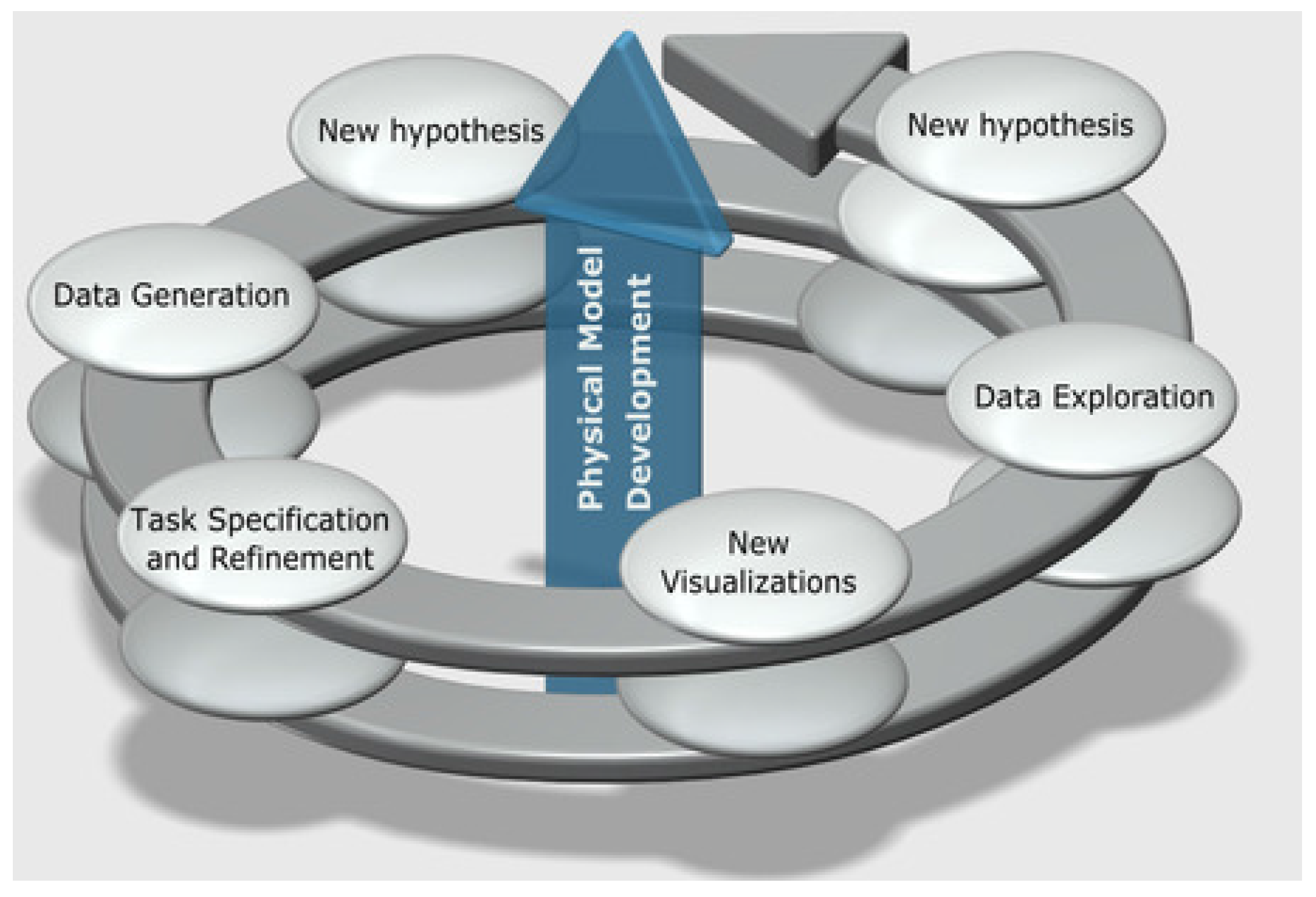
Figure 2.
Our visualization parameter space can be roughly divided into four quadrants micro-level vs. macro-level of detail, ensemble vs. single trajectory). The parameter space can be investigated using several visualization techniques, which are associated with the four identified task groups. To move between the single and the ensemble level, brushing-and-linking is realized using plots.

Figure 3.
Illustration of the different organic solar cell setups. A simple organic solar cell consists of two layers while single (a) or multiple excitons can be considered (b). More complex morphologies reduce interface distances and can also be considered with single (c) or multiple excitons (d). We use a color scheme assigning red to donor material and trajectories and blue to acceptor material and trajectories for all visualizations.

Figure 4.
Screenshot of the system with annotations: It supports the exploration of the trajectory ensemble on different levels of detail. Single trajectories can be selected in qualitative plots (here effective distance a charge has traveled), which then can be inspected as isolated flow lines or with respect to the charge coverage volume within the morphology. An overview of the ensemble distribution provides contextual information.

Figure 5.
The simulation uses periodic boundary conditions, meaning that charges leaving the volume on one side will enter it again on the opposite side. Thus the trajectories are disrupted and the resulting density distribution misleading. The system supports a periodic continuation of the volume to get an untangled representation. The image on the left (bottom) represents raw data in the original simulation volume in contrast to the same data in the extended volume shown on the right. The image on the top left shows a slice through the morphology. The image in the center results from a periodic continuation of the morphology with one selected flow line. The original volume is highlighted by a red square.
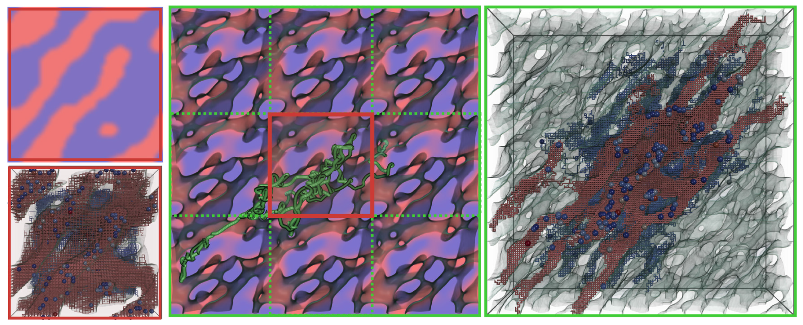
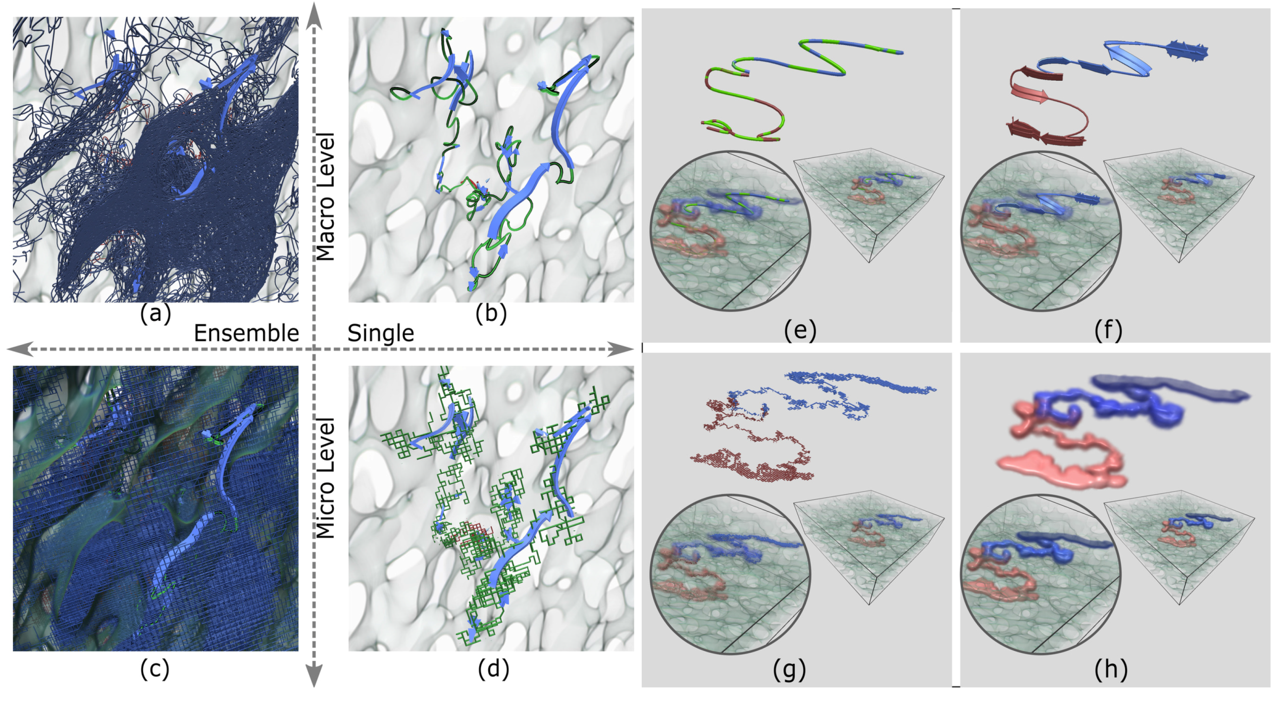
Figure 6.
Trajectory visualization on different levels of abstraction. (a,c) visualization of multiple charge trajectories together with ribbon arrows giving a hint of the general trend of the charge movement. (b,d) show one selected trajectory with micro and macro abstraction level and rendering options. (e–h) show single trajectory abstractions. (e) The stripe pattern is a measure for the effective velocity of the charge. The time the charge needs for one stripe is constant. (f) Arrow representation added to simplified trajectory representation. (g) Direct rendering of raw trajectory represented using tube rendering. (h) Charge coverage volume visualization of single trajectory.

Figure 7.
Interactive plots of morphology composition of single trajectory and ensemble. (a) selected distance measure at a certain time step, with one selected trajectory pair highlighted (b) acceptor-donor ratio along selected trajectory. (c) morphology composition of all trajectories at a specific time step t = 0.4. (d) stack and radial plot for octant acceptor-donor ratio of selected trajectory at specific time.

Figure 8.
Different simplifications can be applied to a trajectory. The red lines are the acceptor trajectories and the grey-blue lines the donor trajectories. (a) One raw trajectory pair, (b) charge flow line with abstraction level in comparison with Gaussian smoothing . The charge flow line is colored with respect to time (same color for donor and acceptor). (c) The escape time measures the time a charge needs to leave the r-neighborhood of a molecule for the first time. (d) charge flow line computation.
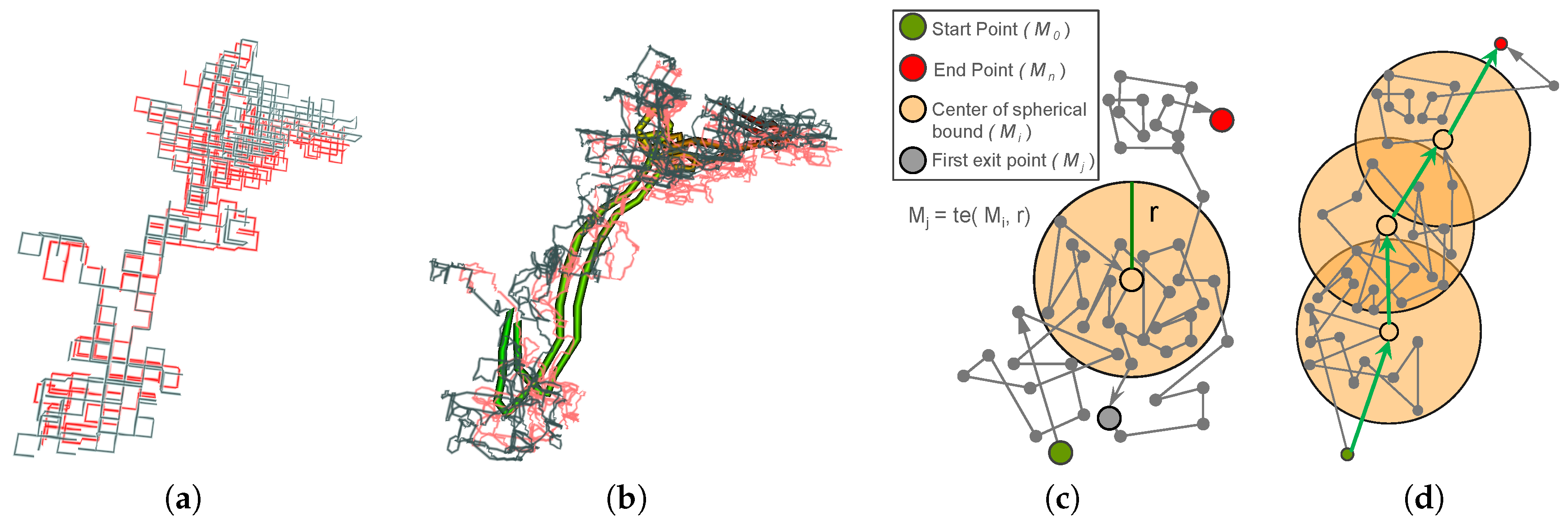
Figure 9.
Top row illustrates various single trajectory representations on a synthetic data. Velocity is color mapped. Bottom row represents ribbon representation, which uses desired curvature range for placement of arrows and co-ordinate frame correction applied.
Figure 9.
Top row illustrates various single trajectory representations on a synthetic data. Velocity is color mapped. Bottom row represents ribbon representation, which uses desired curvature range for placement of arrows and co-ordinate frame correction applied.
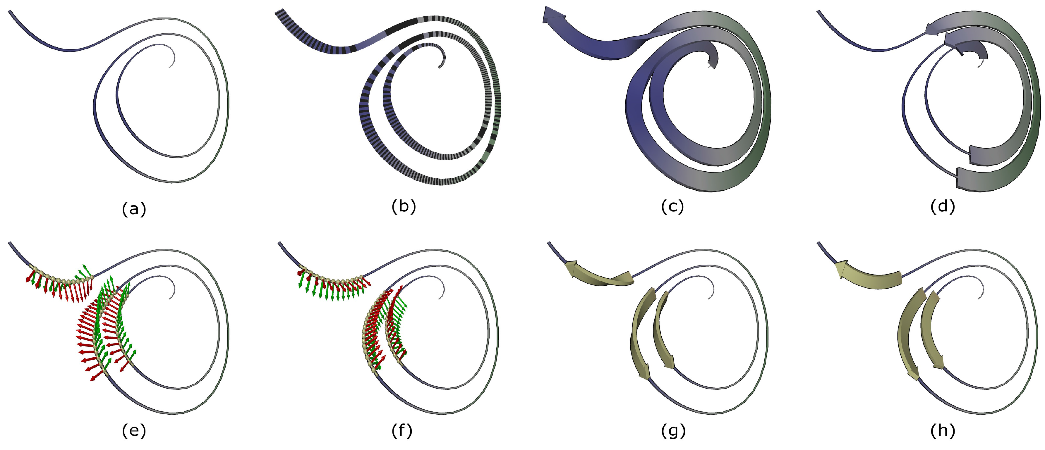
Figure 10.
Scenario 1: Simulation evaluation (SE) of the flat morphology with one charge pair. The images show different rendering options for the entire ensemble (a) trajectories embedded in a charge coverage volume visualization, trajectories reaching the electrode are displayed as spheres colored by time they need to reach the electrode, (b) density projection of trajectories; for one selected trajectory embedded in the charge coverage volume (c) original trajectory colored by progression time (d) flow line displaying the effective velocity as stripe texture.

Figure 11.
The plots of the derived measures for the ensemble highlighting one selected trajectory, the x-axis of all plots is time, which is also encoded in the color of the trajectories. The y-axis are (a) effective distance travelled from start point; (b) distance between the charge pairs; (c) shortest distance to the interface; (d) escape time for a radius of 10 units; (e) parallel coordinates of all the measures (a) through (e).
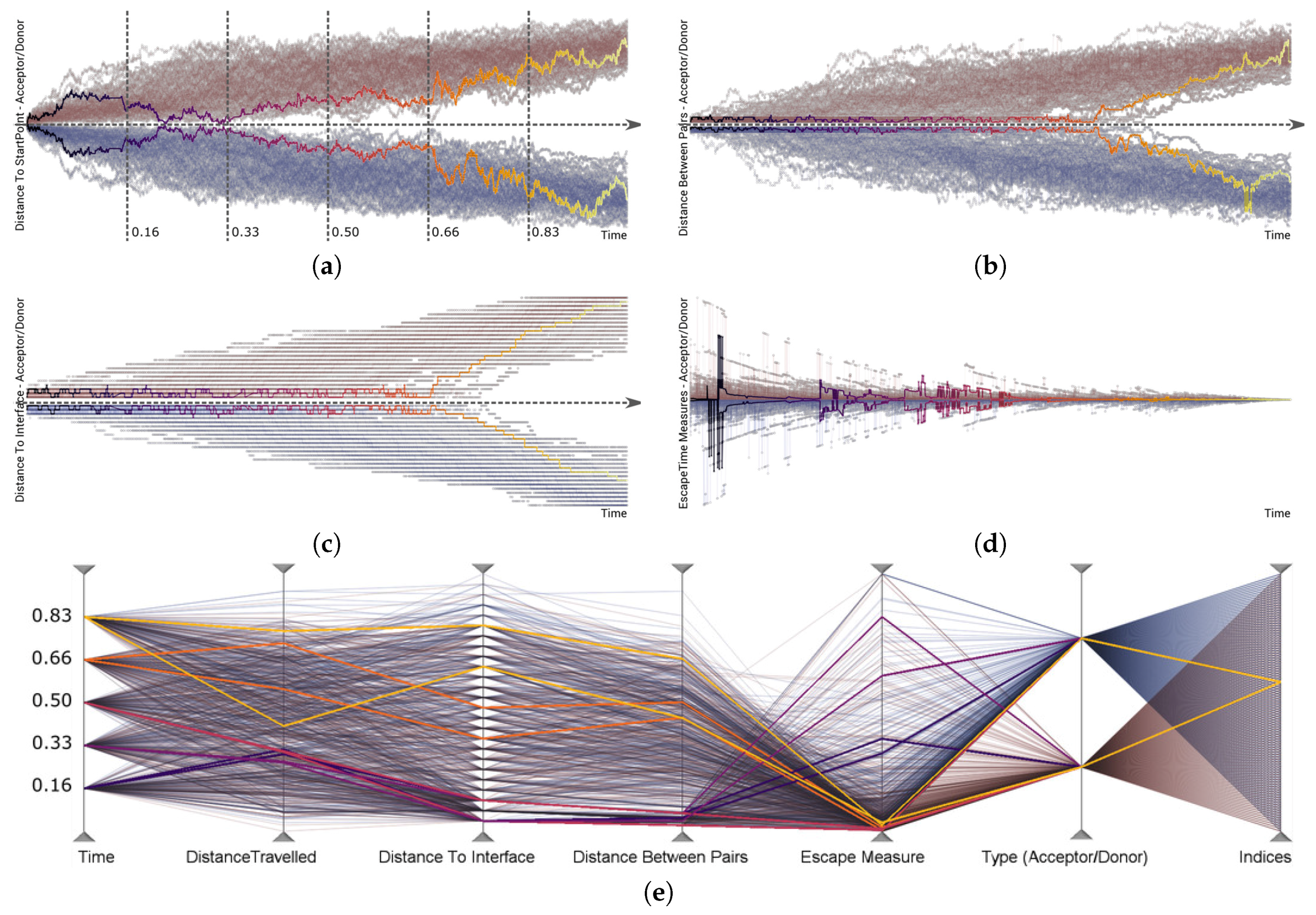
Figure 12.
These images show examples of simulations ((a) Flat Interface, (b) Complex Interface) where the charge transport shows an unexpected behavior. The interaction between the two charges (donor in blue/acceptor in red) is so strong that they stick together for the entire simulation time. They never reach the electrode. The strength of this effect only became visible to the physicist through these visualizations. This observation led to a reconsideration of several simulation parameters and the introduction of the ‘distance between charge pairs’ as additional efficiency measure.
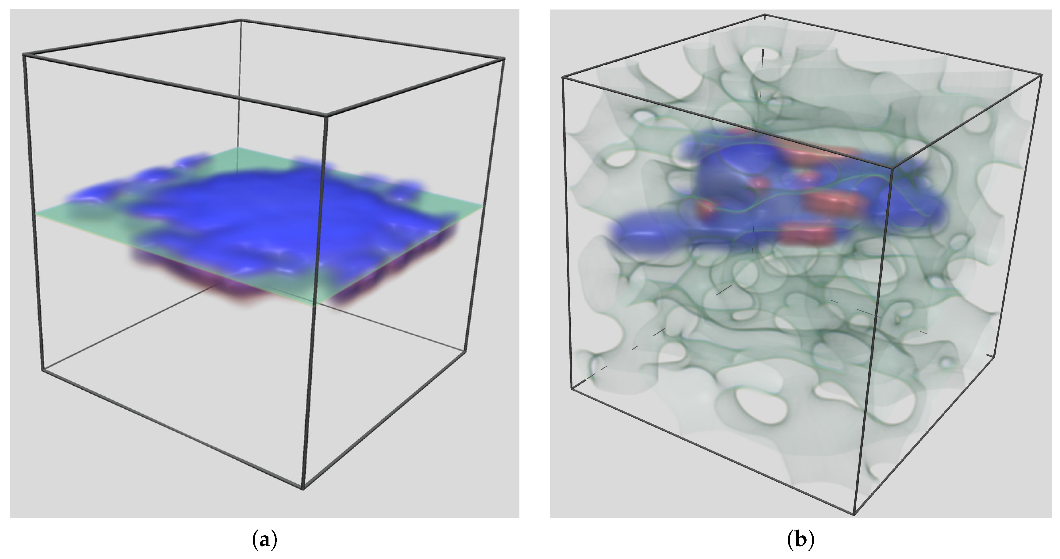
Figure 13.
Overview visualizations for different time steps (columns). The selected time step is highlighted in the plots in the last row as vertical lines. The upper rows show different volumetric visualizations of the ensemble focusing on the different tasks. (a) charge coverage volume within context morphology (Task OE); (b) progression of the trajectory ensemble with time (Task OE, ME); (c) density projection of the trajectory ensemble (Task ME); (d) summary plot distance to start position (Task OE, CI).
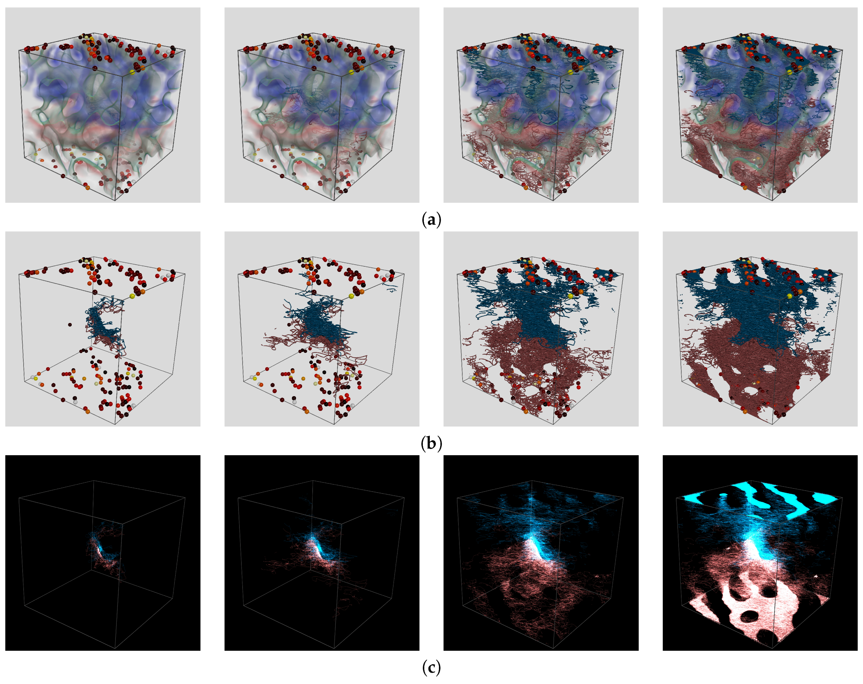

Figure 14.
Three selected charge trajectories are analyzed as above using one of the summary plots. Plot uses time of charge transport along x-axis and y-axis as distance from the start point of charge transport (negative distance is used to differential acceptor and donor pairs in red and blue respectively). This measure allows the user to inspect if charge flow digresses. In this case Trajectory 1 wobbles in a small coverage region for some time before they split apart to reach the electrode. Trajectory 2, on the other hand has shorter transport time for the acceptor and longer transport time for the donor. Trajectory 3 jumps rapidly from start to end. Context rendering.

© 2017 by the authors. Licensee MDPI, Basel, Switzerland. This article is an open access article distributed under the terms and conditions of the Creative Commons Attribution (CC BY) license (http://creativecommons.org/licenses/by/4.0/).
Share and Cite
MDPI and ACS Style
Kottravel, S.; Volpi, R.; Linares, M.; Ropinski, T.; Hotz, I. Visual Analysis of Stochastic Trajectory Ensembles in Organic Solar Cell Design. Informatics 2017, 4, 25. https://doi.org/10.3390/informatics4030025
AMA Style
Kottravel S, Volpi R, Linares M, Ropinski T, Hotz I. Visual Analysis of Stochastic Trajectory Ensembles in Organic Solar Cell Design. Informatics. 2017; 4(3):25. https://doi.org/10.3390/informatics4030025
Chicago/Turabian StyleKottravel, Sathish, Riccardo Volpi, Mathieu Linares, Timo Ropinski, and Ingrid Hotz. 2017. "Visual Analysis of Stochastic Trajectory Ensembles in Organic Solar Cell Design" Informatics 4, no. 3: 25. https://doi.org/10.3390/informatics4030025
Note that from the first issue of 2016, this journal uses article numbers instead of page numbers. See further details here.