
Multidimensional Data Exploration by Explicitly Controlled Animation
by

Johannes F. Kruiger
1, 
Almoctar Hassoumi
2,
Hans-Jörg Schulz
3,
AlexandruC Telea
4 and
Christophe Hurter
5,*
1
Institute Johann Bernoulli, University of Groningen, 9727 Groningen, The Netherlands
2
ENAC/DEVI, University of Toulouse, 31055 Toulouse, France
3
Institute for Computer Science, University of Rostock, 18051 Rostock, Germany
4
Institute Johann Bernoulli, University of Groningen, 9727 Groningen, The Netherlands
5
ENAC/DEVI, University of Toulouse, 31055 Toulouse, France
*
Author to whom correspondence should be addressed.
Informatics 2017, 4(3), 26; https://doi.org/10.3390/informatics4030026
Submission received: 30 June 2017
/
Revised: 1 August 2017
/
Accepted: 14 August 2017
/
Published: 20 August 2017
(This article belongs to the Special Issue Scalable Interactive Visualization)
Abstract
:Understanding large multidimensional datasets is one of the most challenging problems in visual data exploration. One key challenge that increases the size of the exploration space is the number of views that one can generate from a single dataset, based on the use of multiple parameter values and exploration paths. Often, no such single view contains all needed insights. The question thus arises of how we can efficiently combine insights from multiple views of a dataset. We propose a set of techniques that considerably reduce the exploration effort for such situations, based on the explicit depiction of the view space, using a small multiple metaphor. We leverage this view space by offering interactive techniques that enable users to explicitly create, visualize, and follow their exploration path. This way, partial insights obtained from each view can be efficiently and effectively combined. We demonstrate our approach by applications using real-world datasets from air traffic control, software maintenance, and machine learning.
1. Introduction
Information visualization (infovis) aims to leverage user ability to retrieve insight from data representation thanks to the usage of computer-supported, interactive, and visual representations [1]. One of the main challenges of infovis is providing insight into high-dimensional datasets. Such datasets consist of many elements (observations), each having multiple dimensions.
Many visualization techniques for high-dimensional data can be explained as element-based plots. In such a plot, every element of the dataset is depicted separately (and in the same way as the other elements). Examples of such plots are the classical 2D or 3D scatterplots (every element is a point), parallel coordinate plots (every element is a polyline), multidimensional projections, and graph drawings (every element is a graph edge).
When the number of input dimensions is high, no single such plot can be created that shows the entire information present in the input data. This problem is typically solved by generating multiple plots, for various parameter combinations, each of them showing a partial insight. For example, a 2D scatterplot shows the correlation of only two of all the input dimensions, and a graph drawing can generally show an uncluttered view of the input data for only a limited portion of a large graph.
One way to address this problem is to resort to interactive exploration, by allowing the user to create multiple views, each which shows a different part, or aspect, of the data. The problem then becomes how to navigate the (very large) space of all potential views and combine the partial insights provided by them in an efficient and effective way. To address this data exploration issue, we propose a set of innovative techniques where controlled animation plays a central role. Our techniques considerably reduce the exploration effort by allowing the user to directly sketch the exploration path over a visual depiction of the view space created by a small multiple metaphor. This way, a potentially infinite set of intermediate views can be created easily and intuitively. Real-time linking of the view-space navigation and the display of the intermediate views allows one to go forward, backtrack, or change the exploration path. Finally, data patterns found in different views can be selected and interactively combined to generate new views on the fly.
In summary, our contributions are
- a novel representation of the view space based on a small multiple metaphor
- a set of interaction techniques to continuously navigate the view space and combine partial insights obtained from different views
We demonstrate our proposed techniques with the visual exploration of real-world multidimensional datasets represented by multidimensional projections and bundled graph drawings taken from the domains of air traffic control, software maintenance, and machine learning.
The remainder of this paper is structured as follows. Section 2 overviews related techniques for visualizing multidimensional data using element-based plots, as well as techniques for interactive view-space exploration. Section 2.2 introduces the design and implementation of our proposed visualization and interaction. Section 4 shows applications of our techniques to different types of element-based plots. Section 5 discusses our proposal and results. Finally, Section 6 concludes the paper.
2. Related Work
Next, we overview related work to our proposal, structured along three directions: the types of methods used for visualizing element-based plots Section 2.1) and the usage of animation for multidimensional data exploration (Section 2.2).
2.1. Element-Based Plots
Let , , be a dataset containing n-dimensional elements . Further, let be the set of parameters that controls a visualization and the resulting view for the given dataset D. In the following, we use the term visualization to denote the function that creates a depiction (image) of a dataset, and the term view to denote such a depiction. That is, a visualization is a function that inputs datasets, is controlled by parameters, and outputs views. Moreover, for notation simplicity, we will shorten to when the input dataset D is constant and only the visualization parameters P vary, and respectively to when the visualization parameters P are constant but only the input datasets D change.
We define an element-based plot as a 2D drawing consisting of N visual shapes , each mapping a dataset element . Introduced as a concept by Hurter et al. [2], element-based plots generalize many classical infovis techniques: for scatterplots, are nD points and are 2D points; for table lenses, are nD points and are bar-chart-like displays of n numerical values [3,4]; for parallel coordinate plots, are nD points and are 2D polylines; for 2D and 3D scalar fields like color images or 3D data cubes (volumes), are points in , respectively , and are color-mapped pixels, respectively voxels [2,5,6]; and for graphs or trail-sets, are weighted relations or trajectories in some Euclidean space, and are 2D curves [7]. Key to grouping all these visualization techniques under the denomination of element-based plots is the fact that every data item is mapped one-to-one to an independent visual element . As we shall see in Section 2.2, this allows us to manipulate the visualization in very flexible ways.
Below we discuss two types of element-based plots which are particularly important in our context, as they are those on which we validate our animation-based exploratory technique in the remainder of this paper: multidimensional projections and graph drawings.
Multidimensional projections (MPs) are a particularly important type of element-based plots. Here, are nD points (as for table lenses, parallel coordinate plots (PCPs) [8,9], or scatterplots [10]), and are 2D points (as for scatterplots). Hence, MPs are as visually scalable and clutter-free as scatterplots, and more visually scalable and clutter-free than table lenses and PCPs. Moreover, MPs improve upon scatteplots since scatterplots are constructed by using only two of the n dimensions of D, whereas MPs are constructed by considering all n dimensions. As such, scatterplots visually encode the similarity of points according to only two of their n dimensions, whereas MPs encode the similarity according to all n dimensions.
Many MP techniques exist, having various trade-offs between the simplicity, speed, and accuracy of encoding n-D point similarities. They can be grouped in two main classes. Similarity-based projections require only a real-valued similarity (distance) matrix encoding the pairwise similarities of points to construct . In this class, Multidimensional Scaling (MDS) and its variants compute using an optimization process similar to force-based schemes akin to those used in graph layouts [11]. A different approach is proposed by t-SNE [12], which defines the probabilities of picking point pairs in D and minimizes the Kullback-Leibler divergence between those probabilities and those that have the same point pairs as neighbors in the 2D projection. This results in projections that successfully show which n-D points are neighbors to each other, which then helps in visually finding clusters of similar points. In contrast, Attribute-based projections require access to the nD dimensions, or attributes, of the observations to compute the projection . The simplest, and arguably most known, projection in this class is the simple 2D scatterplot created by selecting two dimensions of D. Another well known member of this class is principal component analysis (PCA), which projects on the plane defined by the axes that describe most of the variance in D [13]. However, PCA is notoriously inaccurate in encoding similarity when D resides on highly curved manifolds in n-D. ISOMAP [14] first determines which n-D points are neighbors to build a neighborhood graph, then computes the distances over the neighborhood graph, and finally performs MDS with those distances. Finally, LAMP [15] uses a small number of so-called landmark points that are projected to 2D with a classical MP technique (such as MDS), while the remaining points are arranged around the landmarks using locally affine transformations.
We also note that other classification of MP techniques exist. For instance, these can be grouped into global (scatterplots, PCA, star coordinates [16,17], orthographic star coordinates [18], biplots [19,20], radial visualizations [21,22]), and local (LAMP, LLE [23], t-SNE [12]). Global techniques use the same transformation to project all points to the target (2D) space. They are simpler and faster to compute but may generate large projection errors. Local techniques may use different transformations for different point neighborhoods. They are in general more complex and slower than local techniques, but they preserve the so-called ‘data structure’ better after the projection than local techniques.
Among all the aforementioned multidimensional visualization techniques (scatterplots, table lenses, PCP’s, and projections), the latter are the most visually scalable and clutter free, as they map an n-D point to a 2D point. However, projections are fundamentally weak in accurately showing similarities between n-D points for the entire input dataset D [24]. As such, given such a dataset D, there is typically no single projection that can faithfully show all patterns D. We shall show in Section 4 how we effectively address this problem by interactively combining insights obtained from different projections of a given dataset D.
Graph drawings (GDs) are a second important type of element-based plots. In detail, a graph is a dataset with nodes and edges . Both nodes and edges can have data attributes, thereby making D a multidimensional dataset. A graph drawing is a visualization , where is typically a 2D scatterplot of points . is typically created by embedding methods such as force-directed layouts [25] but also, as shown recently, multidimensional projections [26]. can be a set of straight line segments . However, can also be 2D curves, as follows. Drawing large graphs (thousands of edges or more) with straight lines easily creates massive clutter which renders such drawings close to useless. One prominent method to simplify, or tidy up, such drawings is to bundle their edges, thereby trading clutter for overdraw—that is, many bundled edges will overlap in . This creates empty space between the edge bundles which allows one to easily follow them visually, thereby assessing the coarse-scale connections between groups of related nodes in more easily than in an unbundled drawing. The drawback of bundling is that individual edges in are harder to distinguish due to the overlap. Numerous edge bundling (EB) methods exist [27,28,29,30,31,32]. However, as a recent survey points out [7], no such method is optimal from all perspectives. For instance, some methods offer a very precise control of the shape and positions of the bundled edges, but only handle particular types of graphs [27,32]. Other methods can handle graphs of any kind and are very scalable but offer far less control on the resulting look-and-feel of the bundled drawing [28,29]. Yet other methods fall in-between the above two extremes but generate a very wide set of drawing styles [33].
2.2. Navigating Multidimensional Data Visualizations
Exploring the space of visualizations that one can create for a given multidimensional dataset is a wide topic. Several technique classes exist to this end, as follows.
Animation is a prominent technique that supports exploring the parameter space and the related view space . Animation has a long history in data exploration [34,35]. In this context, animation corresponds to a (smooth) change of the visual variables used to encode the input data [1,36].
Animation has proven to help users transition between visual configurations [37] while maintaining the mental map of the data exploration [38]. The simplest form of animation, used by virtually all visualization tools, lets an user vary the value of interactively by a classical user interface (GUI) while watching how the changes. While simple, this type of animation does not ‘guide’ the user in the exploration of the parameter space and the related view space in any way. Within the scope of multidimensional visualization, parameter-space animations include rolling-the-dice [39], where the user controls the plane on which the multidimensional data is projected; the grand tour [40], where a large sequence of 2D projections are displayed from a multidimensional dataset in a flip-book manner (the parameters P controlling projection-plane orientation in nD being varied randomly); the class tour [41], which refines the grand tour so as to generate projections which preserve class separation of the data points; combinations of the grand tour with projection pursuit [42] (the parameters P controlling the projection-plane orientation being varied along the derivatives of the so-called projection pursuit index, so as to drive the tour through interesting projections); and drawing faded trails that connect two consecutive views in a tour to give a feeling of how the projection plane changed in between [43]. A limitation of most grand tour techniques is that they only handle attribute-based projections [44].
Small multiples: Explicitly showing a sampling of partially addresses this issue. One can show a history of views obtained for various parameter settings used in the exploration so far. The history can be shown as a linear, grid-like, or hierarchical set of thumbnails depicting , a metaphor also called ‘projection board’ [44]. By clicking on the desired thumbnail, the user can go back to the corresponding state and associated view , and continue exploration from there. Approaches that utilize such a methodology are Ma’s Image Graphs [45] and Elmqvist et al.’s Data Meadow [37]. Most projection pursuit variants also fall into this category [42,46], every view being one deemed ‘interesting’ from the perspective of the projection pursuit index, a metric which typically measures the distance from a given projection to an uninteresting generic Gaussian-like scatterplot. However, a limitation of most projection pursuit variants is that, just like grand tour variants, they require attribute-based projections [44]. Projection pursuit methods have been recently enhanced by limiting the number of interesting views to [47].
Many scagnostics techniques also use the small-multiple metaphor to show interesting projections, where interest is defined in a wide variety of ways [48,49,50,51]. Besides using the exploration history, the views can be picked by optimizing for diversity of this set, by subsampling an initial large random sampling of , or by iteratively refining a given set of views to improve their diversity [52]. Other methods add aesthetic constraints, such as a symmetry score, to exclude unsuitable views right from the view set [53]. The thumbnails can also be placed in 2D by projecting the set of presets by using Multi-Dimensional Scaling (MDS) methods [52,53], similar to those discussed in Section 2.1, or simply arranging them in increasing distance to the currently shown one [54]. Other arrangements use a regular grid layout that allows performing additional view transformations by a spreadsheet-like metaphor [55]. All above metaphors assume a small set of preset views , so that they can all be displayed simultaneously as thumbnails without taking too much screen space. If users are not satisfied with these proposed views, they can usually only adjust the parameters that generated them in the hope to get better ones. Another way to refine the set is to mark the views that are closest to what the user has in mind and supersample around such ‘interesting’ views to get better ones [56].
Preset controller: In contrast to small multiples, Van Wijk et al. [57] show several values of specific parameter-sets by a 2D scatterplot , where is the projection of the point . Next, one can manipulate a point of interest , or the scatterplot points , and generate a corresponding parameter-set value by using Shepard interpolation of the values based on the distances . While the preset controller is very simple to use and is scalable in the number of parameters , it does not explicitly depict the view space but, rather, only an abstract view of the parameter space .
Direct manipulation: Animation can be also controlled directly in the view space rather than in the parameter space . For this, the user directly manipulates the depicted visual elements in to modify the parameters P. Examples of such manipulations are deformation, focus-and-context, and semantic lens techniques, all of which typically linearly interpolate between two parameter-set values and and show the corresponding animation of to . Such animations have been applied to large element-based plots such as bundled graphs and scatterplots [6,58]. Smooth real-time animations of large datasets have been made possible by using GPU-based techniques [59]. For multidimensional projections, we have the following direct manipulation techniques. Control-point-based projections, such as LSP [60], PLMP [61], generalized Sammon mapping [62], hybrid MDS [63], and LAMP [15], allow users to interactively (dis)place a small subset of , called control points, on the 2D view plane, after which they arrange the remaining points around these controls so as to best preserve the nD data structure. This effectively allows users to customize their projections, at the risk of creating visual structures that do not relate well to the data. Targeted projection pursuit (TPP) [64] allows users to drag elements in a multidimensional projection plot to, for example, better separate classes. From the resulting scatterplot , it seeks the parameters P for an actual projection that is close to . While powerful as an interaction mechanism, TPP limits itself to only linear projections. Recently, ProjInspector use a preset controller, where the k presets correspond to user-chosen DR projections , . When one drags the point of interest in the controller, the tool generates a view that blends all by means of mean values coordinates interpolation [44]. ProjInspector is arguably the closest technique to the one we present here, as such, we will discuss the similarities and differences in detail in Section 5.
Interaction techniques: All the above-mentioned visualization techniques use a mix of interaction techniques to enable exploration. While these are not specific to multidimensional data exploration, it is worth mentioning them here, as they next allow us better placing our contribution. First, as already explained, the parameters P can be changed by means of classical GUIs: the elements of the view , the control points of a preset controller [44,57], and the control points of a projection [15,60,61,62,63] are changed by simple mouse-based click-and-drag. Techniques can be next classified as single-view or multiple-view. Single-view techniques are either interaction-less, e.g., some grand tour and projection pursuit variants, or require direct manipulation in the single view, as explained earlier. Multiple-view techniques display several views of the data. If direct manipulation is implemented in one view , then the elements undergoing change should be updated in all other views – a well-known technique under the name of linked views [65] or coordinated views [66]. Depending on the exact semantics of the views, either unidirectional or bidirectional linking can be used [67]. For instance, a preset controller is unidirectionally linked to the data view(s) it controls. Finally, brushing and selection are ubiquitous techniques for exploring the view space, by showing details of the data element under the mouse and click-and-drag (typically) to select a subset of for special treatment, respectively [68]. We will use all these techniques in the design of our exploratory visualization in Section 2.2.
Other approaches: Visualization presets have also been investigated for graph datasets [69]. Separately, exploratory visualization approaches have used the view space in a foresighted manner to sketch possible next steps along the visual exploration path. Several such approaches exist, which can be subsumed by the term ‘visualization by example’ [70]. All such approaches allow one to select a desired view from a range of candidates, the main distinction being how these candidates are picked from the view space and how is presented to the user.
Our proposal: We combine several of the advantages, and reduce some of the limitations, of the above-mentioned techniques for navigating a view space constructed from a high-dimensional dataset D by means of a parameter space , as follows:
- Genericity: We handle all types of element-based plots (Section 2.1), e.g., scatterplots, graph/trail drawings, and DR projections, in an uniform way and by a single implementation.
- View by example: We provide an explicit small-multiple-like depiction of the view space .
- Continuity: We allow a continuous change of the current view based on smooth interpolation between the small-multiple views without having to bother about understanding the explicit abstract parameter space . This allows generating an infinite set of intermediary views in .
- Free navigation: The view generation is in the same time controlled by the user (one sees along which existing views one navigates) and unconstrained (one can freely and fully control the shape of the navigation path).
- Ease of use and scalability: We generate our intermediary views by simple click-and-drag of a point in the view space; these views are generated in real-time for large datasets D (millions of elements).
- Control: Most importantly, and novel with respect to all approaches discussed so far, we propose a simple mechanism for changing only parts of the current view, while keeping other parts fixed. This enables us to combine insights from different views on-the-fly, to accumulate insights on the input dataset D.
3. Proposed Method
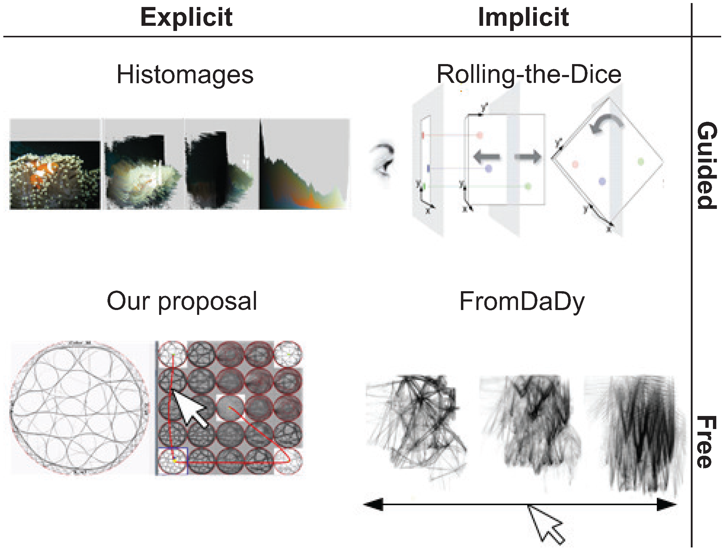
We next present our animation-based exploration of visualization spaces for element-based plots, following the discussion in Section 2. To better outline the added-value of our proposal, we first classify the types of such animation-based explorations along two axes that explain how the transition between views in can be created: explicit vs. implicit, and guided vs. free, as follows (see also Figure 1).
The first axis (vertical in Figure 1) describes the type and number of preset views between which the user can navigate, and has two values (options):
- Guided: The set of preset views between which the user can choose is limited by construction, and depends on the dimensionality of the input dataset D.
- Free: The set of preset views is fully configurable by the user, who can choose any number and type of views in to animate between.
The second axis (horizontal in Figure 1 characterizes how the user can control the animation during the transition between two views and , and has tho values:
- Implicit: Once the transition (animation) between and is triggered by the user, the generation of intermediate views between and happens automatically (usually via some type of linear interpolation). The user can specify and , but not the path in the view-space along which the animation evolves nor can he slow/accelerate/pause the animation.
- Explicit: The user can choose the path along which the animation evolves, and also the speed thereof.
To clarify the above, some examples of existing animations follow.
Implicit and guided transition: Rolling-the-dice [39] is a metaphor of a 3D rolling die which allows smooth transitions between 2D scatterplots obtained from an nD dataset. The preset views are implicitly defined by the pair-wise combinations of data dimensions in the input dataset D ( in total). The transitions are automatic linear interpolations between two such scatterplots.
Implicit and free transition: In FromDady [58], the user can interactively define views to animate between, based on desired combinations of the dataset’s attribute-pairs. In contrast to ScatterDice, the user can control the transition speed and direction ( to or conversely) with a mouse drag gesture. However, the set of preset views is given by the pair-wise combinations of dimensions in the input data. Moreover, the transition is not entirely free, although one can control its direction and speed, its path is still a linear interpolation between and .
Explicit and guided transition: The user can define an open set of preset views that can be interpolated. For example, in the preset controller, these views are arbitrary parameter-sets that generate corresponding views [57]. However, the transitions between views are still automatically determined, typically by linear interpolation. Further examples hereof are [2,6,71].
Explicit and free transition: To our knowledge, no existing technique allows freely defining both the endpoints and the controllable interpolation path for the animation. Our proposal, described next, fills this gap.
3.1. Our Proposal
Our key idea is to combine the main strengths of the explicit and free animation methods existing in prior work, in an efficient and effective way. To this end, we choose to
- Allow one to freely sketch the interpolation path between two such view presets , in an interactive and visual way (as in [57]), rather than automatically controlling the interpolation via a linear formula.
We proceed as follows. Figure 2 illustrates the process for a multidimensional dataset D that we visualize using multidimensional projections, which are introduced in Section 2.1. We proceed by allowing users to specify any (small) set of views for the given dataset D. These can be created either by the same visualization method, but using different parameter values , or by completely different methods. The only restriction is that these should be element-based plots, i.e., consist each of N visual elements , , one for each data element . We organize these view presets in a simple square grid, much like [55], to minimize the used screen space to display them (see Figure 2b).
As explained in Section 2.2, manually generating a rich set of view presets can be delicate. Typically, one starts with a small set of just a few salient view presets, for instance, one for each type of visualization method considered for a given dataset. In our running example in Figure 2, we have five such presets, corresponding to five multidimensional projection methods (PCA [13], Isomap [14], LAMP [15], MDS [11], and t-SNE [12]). In general, these views can be very different. In other words, they are a very sparse sampling of the rich view space . We do not know what lies in between, so, navigating between them can be unintuitive.
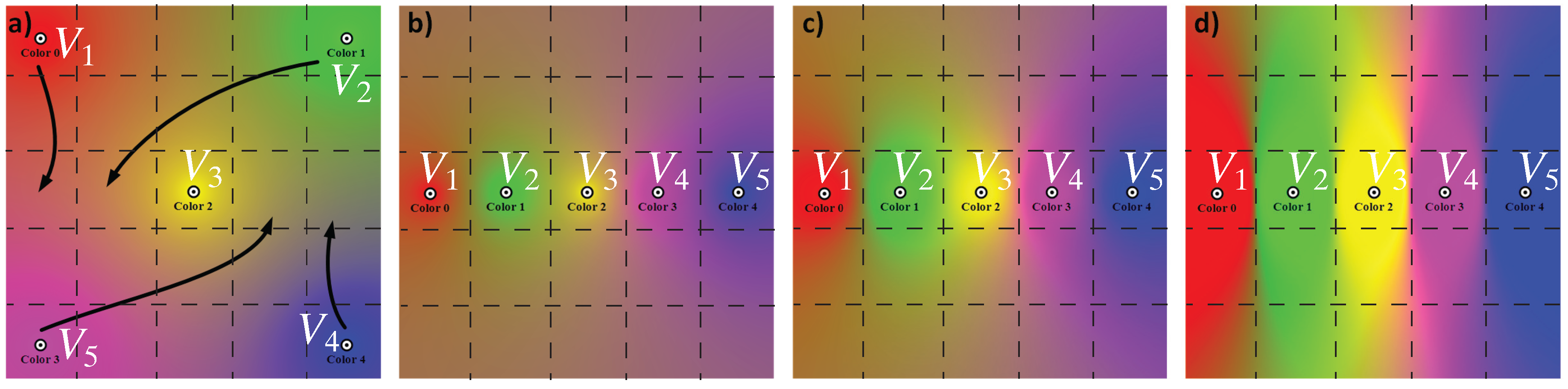
To alleviate this, and also to realize our animation-based exploration mechanism presented next, we propose a view-space interpolation mechanism, as follows. Let be a point in the 2D grid space where we place the view thumbnails. Placement of thumbnails can be freely specified by the user, based on perceived similarities between the views and following the design of the original preset controller [57]. Let now be the centers of the thumbnails in this grid. We use an Inverse Distance Weighting (IDW) method, such as the Shepard method [72], to compute the elements of the interpolated view at position x as:
Here, denotes 2D Euclidean distance, and is the interpolating basis function controlled by the power parameter . Typically we use , which leads to classical inverse quadratic Shepard interpolation. Key to our idea is the fact that all element-based plots consist of sets of simple graphical elements such as dots or line segments. These can be thus easily interpolated using Equation (1). If desired, different types of (smooth) scattered-point interpolation can be used, such as radial basis functions or mean values coordinates [44].
Having now a way to interpolate between views, we supersample the view space to generate additional views between the presets provided by the user and display these additional interpolated views along with the provided ones. Figure 2c shows this: here, from the original five presets, we create an additional number of 20 presets, yielding to a total grid of views. The interpolated views now give a better idea of what the animation-based exploration will produce when we will navigate the view space between the originally provided views.
Having now the densely-sampled view space, we provide an interactive way for users to generate arbitrary views. For this, the user drags a so-called focus point x over the thumbnail grid. Note that x can assume any pixel position over the extent of the grid, i.e., is not constrained to the centers of the grid cells only. We then generate the view corresponding to this point, using the same interpolation (Equation (1)) as for the view-space supersampling, based on the distance of x to the centers of the originally-provided views (Figure 2d), and display this view at full resolution in a separate window (Figure 2e).
As noted, the original views can be freely arranged over the thumbnails grid. This, and changing the power p in Equation (1), offers a flexible way of specifying how the original views are mixed to yield the view at some position x. To better understand this, Figure 3 shows the effects of these two changes. Here, we have five views , arranged on a five by five thumbnails grid. Each entire view (and thus thumbnail) is simply a colored pixel in RGB space, for illustration purposes: = red, = green, = yellow, = purple, = blue, and = purple. As such, we can render the interpolated views at all the positions x over the thumbnails grid. In other words, the color images in Figure 3 show the entire view space that can be generated from the five presets, something we cannot do, of course, for actual views of complex datasets. Figure 3a shows how the interpolated views (colors) smoothly vary between the five presets. Figure 3b shows how the view space changes if we drag the five preset views to be in the same horizontal grid row, as indicated by the arrows in Figure 3a. Finally, Figure 3c,d shows the effect of changing the value p from the default used in the first two images (a,b) to and , respectively. This allows us to control the shape of the zone of influence of each view over the thumbnails grid.
Several types of exploration of the view space are now possible using these mechanisms (see also Figure 4). The simplest is to click on one of the cells of the thumbnails grid. This sets the current view to the preset view corresponding to that cell (Figure 4a). Separately, one can drag the mouse to follow a path in the view space. Making this path pass through a number of preset views essentially constructs a ‘visual story’ that leads the user through the insights provided by these views, in visiting order (Figure 4b). In this sense, our technique is a specific instance of the design space model proposed in [73]. We offer the possibility of saving such a path and explicitly drawing it atop the thumbnails grid. This allows one to revisit an earlier-inspected view in the view space, thus, to backtrack the exploration, following well-known principles in information visualization [74] (Figure 4c).
Besides arranging the preset views in the thumbnails grid and interactively dragging the focus point over the grid to generate a current view, we provide a third (and last) interaction mechanism called the lock tool. This allows the user to select points in the current view by lasso selection (see Figure 2e). The underlying data points corresponding to these selected points are then excluded from the interpolation in Equation (1) when the focus point is dragged. This offers the possibility to the user of locking interesting visual patterns that have been discovered, during the animation, in one or several current views. This way, the user can effectively interactively create a custom view that blends insights obtained from different parts of the exploration process.
3.2. Implementation Details
We next detail the implementation of our proposal. Since we heavily rely on animation, we need to be able to generate the current view , by using the interpolation in Equation (1), in real-time for large element-based plots containing hundreds of thousands of points or more. We developed our exploration tool in C# using .NET 4.5 and using OpenGL for rendering. To support scalable animation, we investigated different solutions. We first found that the fixed OpenGL pipeline (used earlier for similar animation-based explorations [2]) and the render-to-texture OpenGL extension (also used earlier for similar goals [58]) do not provide enough scalability. We next investigated the use of the OpenGL transform feedback (also used earlier for similar goals [6]). This technique addresses scalability issues and is faster than the render-to-texture solution. However, the implementation becomes quite complex, as one has to code all the interaction and interpolation in a fragment shader whose code becomes hard to manage. We therefore explored another solution based on coding Equation (1) in NVIDIA’s CUDA parallel programming language. This solution proved to be even faster than the transform feedback one, while allowing for a simple implementation too. As a result, our tool can generate fluent animations of datasets having up to one million visual elements (points) on a modern GPU.
4. Applications
We now demonstrate the working of our proposed animation-based exploration techniques by applying them to two types of element-based plots—multidimensional projections (Section 4.1) and bundled graph drawings (Section 4.2). Additional video material illustrating our animation-based exploration is available online [75].
4.1. Multidimensional Projections
Our datasets D are here tables where each row corresponds to an observation and each column to a different (numerical) property measured for the respective observations. Hence, D can be seen as point sets in a high-dimensional space. The preset views we start with are various projections of such nD datasets to two dimensions. We consider three such datasets, and associated projections, as follows.
4.1.1. Software Dataset
In this dataset, observations correspond to software repositories from SourceForge.net. The dimensions are different quality metrics of the software repositories, such as the number of lines per method, coupling between objects, and the cyclomatic complexity of methods. For each repository (observation), metric values are averaged over all its units of computation (classes, methods, files). Details on these metrics and the data are available [76]. Additionally, every observation is labeled by its type (e.g., small library, large library, monolithic application).
One interesting question for this dataset is whether projections can help us separate repositories of one kind (say, small class libraries) from those of other kinds (say, large monolithic systems). Note that none of the metric values present in the data contains absolute size information.
Figure 5 shows a five by five thumbnail grid based on the Isomap, LAMP, t-SNE, PCA, and MDS projections. Here and next, we chose these projections as they are well-known in the literature and often used in practice when analyzing multidimensional data. The projected points are colored based on their class (repository kind) attribute, which is not used by the projection. In the thumbnails, but even more so when interactively navigating the view space by clicking anywhere in the thumbnail grid, we see that no single view can separate well points of one color (class) from the others. The view that yields the best separation is t-SNE, also shown in detail in the right image in Figure 5. However, even in this view, we see no clear segregation of points of one class from the others. We conclude that the 11 recorded metrics are not a good predictor of the type of software system in a repository—in other words, systems of different kinds can have similar qualities, and conversely. Interestingly, the same result was noted by the original paper that analyzed this dataset [76], which did not use multidimensional visualization. Separately, a different work also showed that using 2D projections cannot achieve the desired separation but that such a separation is better possible using a 3D projection [77].
4.1.2. Segmentation Dataset
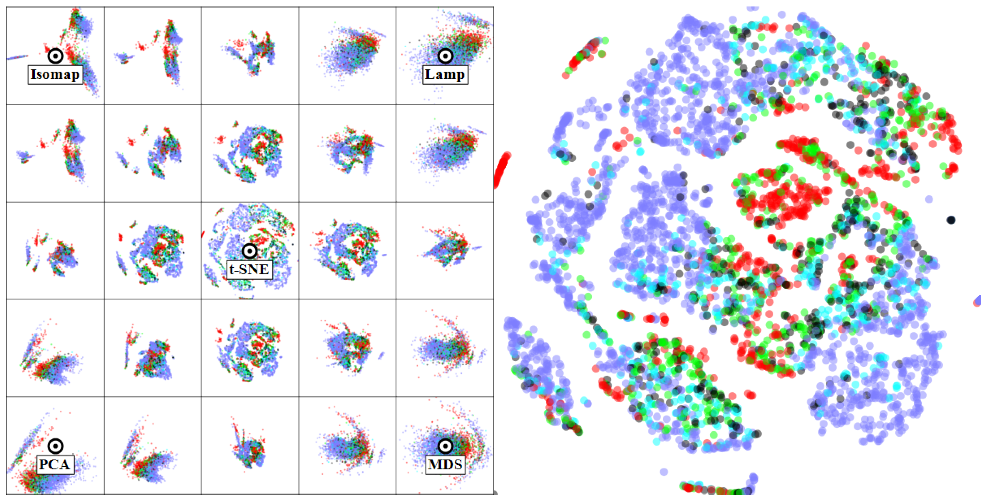
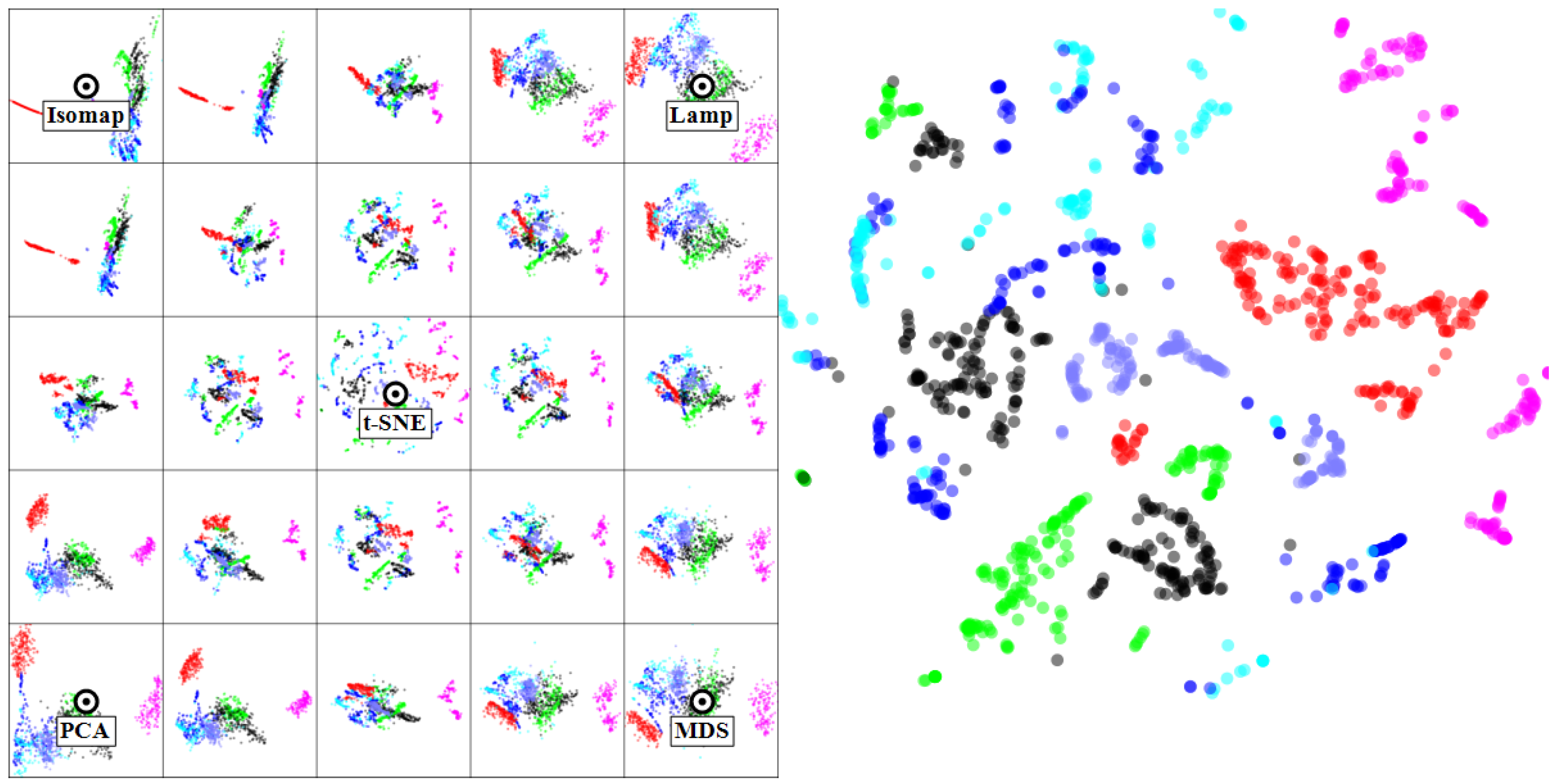
In this use-case, the dataset D is a set of seven images. Every dataset element corresponds to a three by three block of pixels from one of the images, that is manually labeled into six classes (e.g., brickface, sky, grass, etc). Each of the elements has 17 dimensions which describe image features computed on the block of pixels. This dataset is well known in the machine learning literature , in the context of designing classifiers able to predict the six classes from the 17 measured dimensions [78]. To do this, one way is to engineer discriminating features using the raw 17 ones present in the data. Projections can help us in determining how good the engineered features are: if we find a projection where same-class points are well separated into clusters then the features that the projection has used as input are a good start for building a good classifier [79].
Figure 6 shows our method applied on this dataset, with the right image showing the t-SNE projection. As visible, several of the intermediate views (between the five presets) are able to separate well one or more classes from the others but no single view can do this for all classes. More interesting, we see that different views can separate well different classes. This is a key insight that we interactively refine further (see Figure 7). We start from the central t-SNE view (a). Next, we see in the tumbnail grid that the LAMP view separates cluster 1 (red) very well from the rest (f). We navigate to , where we can easily select the red points and lock them for transitions. (b) From here, we notice another view (, image (g)) where clusters 2 (gray-blue) and 3 (purple) are well separated. We navigate from to . Since cluster 1 is locked, it will stay well separated during this process. We now can easily select clusters 2 and 3 and lock them. Next, we repeat the process by finding where we can separate cluster 4, and finally , which separates the two remaining clusters 5 and 6. The entire process takes around two minutes and requires only basic click, drag, and brush mouse interaction. The iterative lock-and-view-change process is equivalent with an iterative classifier design where one finds specific features (given by the projections corresponding to the views ), which are good to separate one or a few classes from the rest. While we have not created and tested such a ‘cascading’ classifier, doing so should be relatively straightforward now that we know which configurations are good in separating one class from the rest, and the order of these configurations.
4.2. Bundled Graph Drawings
Graphs are used to encode large relational datasets, such as the dependencies between components in a software system. As outlined in Section 2, a graph drawing can also be seen as an element-based plot, where the drawn edges are the elements. As also explained there, edge bundling (EB) is an established effective instrument for reducing clutter in large graph drawings, allowing one to follow easier the coarse structure of a graph. However, we have outlined that no single bundling method is ideal. The situation here is very similar to the visual exploration of multidimensional projections: we can generate a right set of bundled drawings; each drawing may be good for conveying partial insights in the input graph; but no drawing is optimal in this respect. Hence, having a way to merge the insights obtained from multiple EB drawings is useful.
We can use our method to mix several drawings created by different EB methods, as follows. For this, we consider a dataset having 1024 nodes, which are functions of a software system, and edges, which model function calls. The nodes are laid out in a radial way (for details, see the radial dataset in [28,29]). Figure 8 (b) shows the unbundled graph, where one clearly cannot see any structure. The thumbnail grid is based on five presets, containing the bundling of the graph by the KDEEB method [29] (images (c) and (d); we used here two parameter sets for KDEEB, the first by pre-clustering graph edges based on their spatial similarity, and the second by using no clustering), the SBEB method [28] (image (e)), and the ADEB method [30] (image (f)). We start our navigation from the unbundled view to view 2, where we see three bundles which are well separated from the others. As such, we want to keep these, so we lock them. We continue the same process by going through views 3 to 5, each time locating bundles that are well readable in the current view, and locking these. The final image (g) shows the locked bundles in the context of a view that is very close to the original unbundled graph. This represents thus a ‘patchwork’, or mix, between four types of bundling, applied selectively on different parts of the data and the original data. Obtaining such a view is not possible by using any of the EB algorithms in existence.
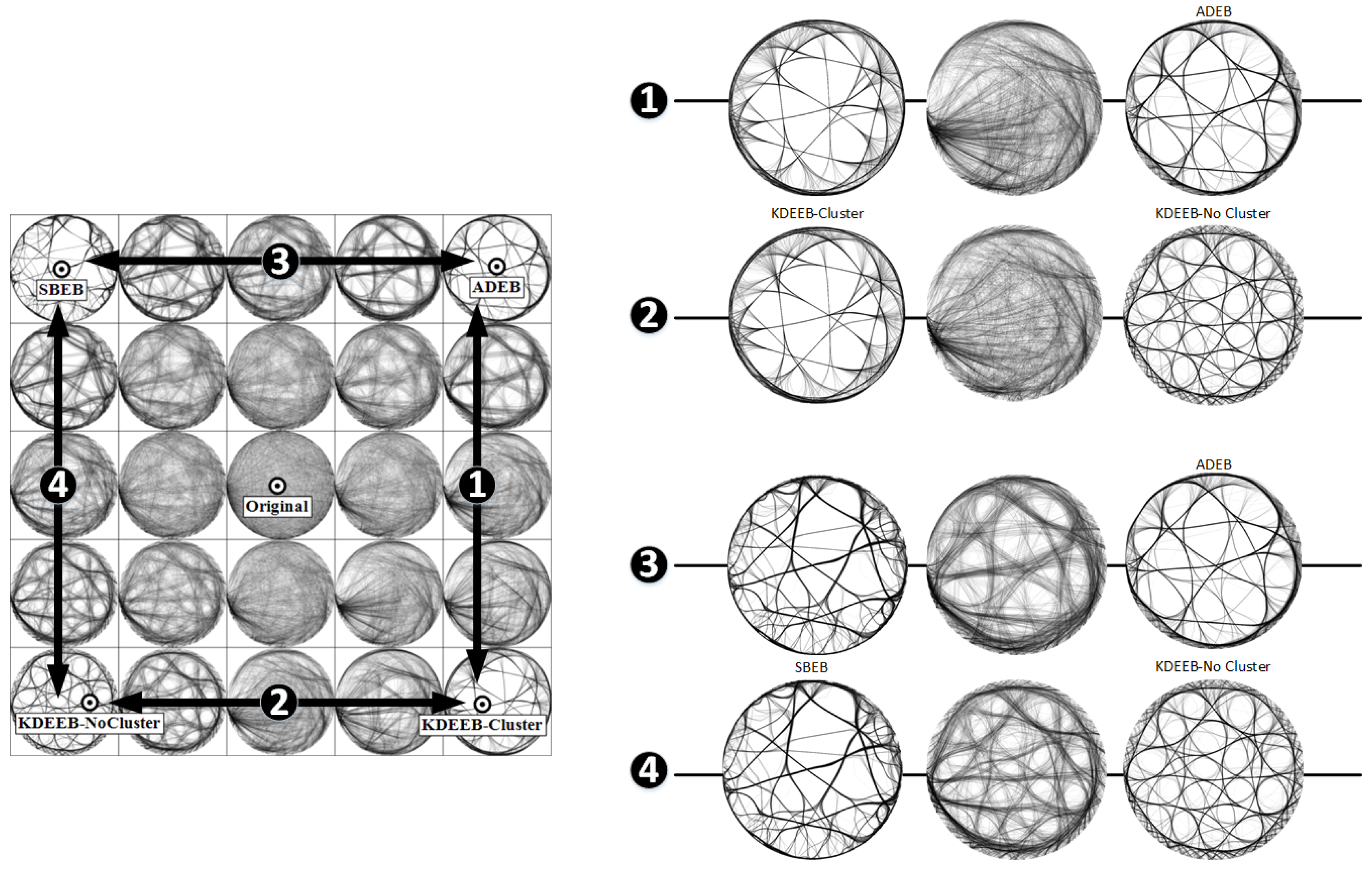
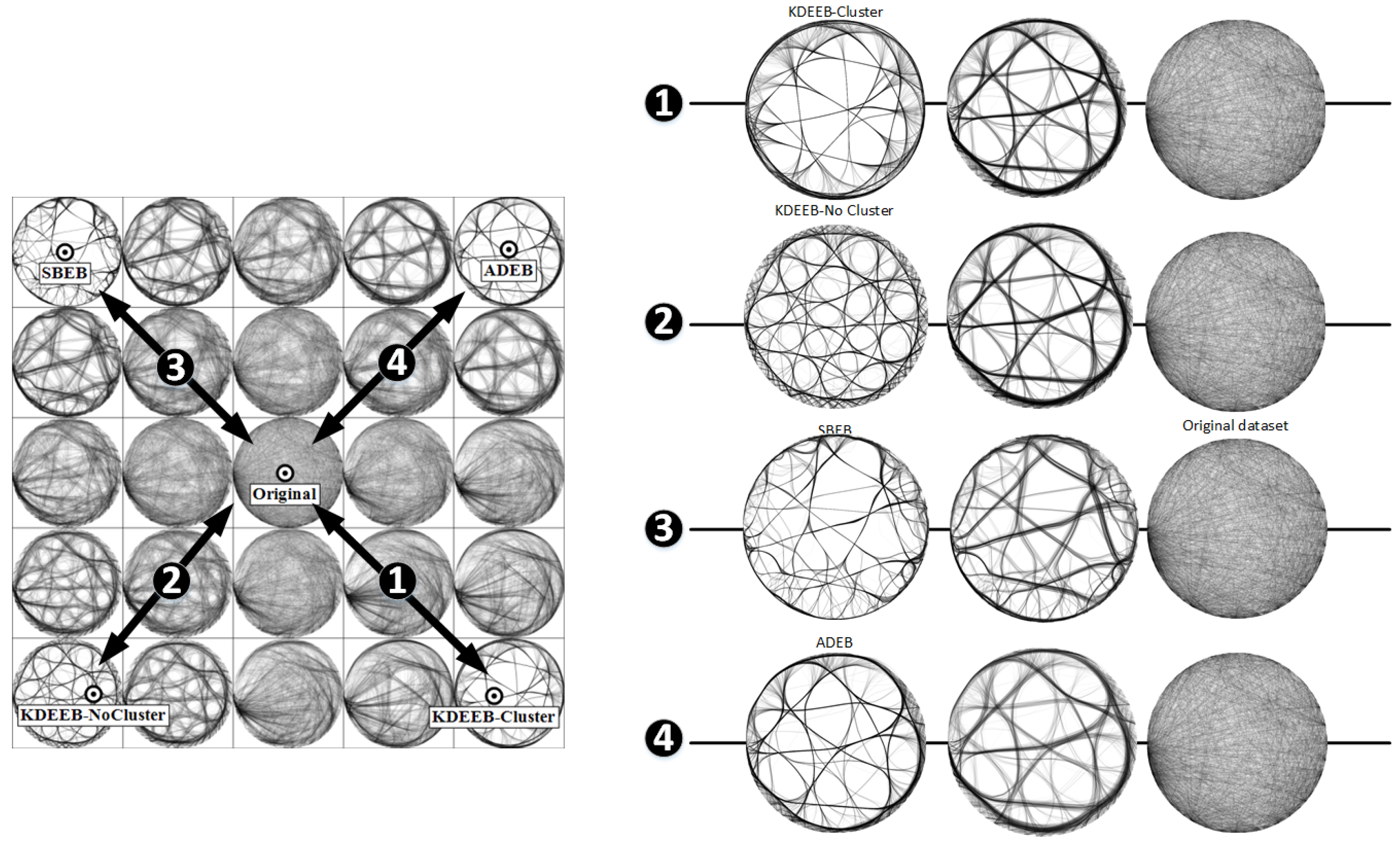
A second use-case regards the visual comparison of EB techniques. Given several such techniques (or results of the same technique but obtained for different parameter values), an important question is which are the main differences between them. Knowing this helps users in, for example, assessing which techniques behave similarly and thus can be substituted for each other in an application. Figure 9 shows how we can answer this question. We use here the same thumbnails grid and dataset as in Figure 8. However, we only perform four simple navigations, by going several times to-and-fro between the four preset views in the grid corners. The right image in Figure 9 shows intermediate frames during these animations. We see here that going from SBEB to ADEB or from SBEB to KDEEB-NoCluster creates relatively structured in-between frames. Hence, the methods SBEB, ADEB, and KDEEB-NoCluster provide similar layouts in terms of their visual signatures. In contrast, going from KDEEB-Cluster to KDEEB-NoCluster or to ADEB creates intermediate views that look completely messy. This tells us that the KDEEB-Cluster method has a very different visual signature (style of result) than the other methods. A second use-case for this scenario is to compare the quality of two EB techniques A and B: if we know that, for example, A is of high quality, and our animation shows only small differences between A and B, then we can infer that B is also of good quality (the converse being also true).
In the examples above, we had as input data general graphs and, as such, we used general-graph bundling methods such as KDEEB, SBEB, and ADEB. Hence, even if the nodes are laid out on a circle, the bundling methods we use should not be confused with, for example, HEB [27]; the only resemblance is that both bundling methods read an input graph whose nodes were laid out on a circle. However, this does not mean that we cannot use HEB or any other method for hierarchical graphs as a preset view, as long as the input graph is hierarchical, of course.
As a final note, we remark that our animation technique provides, for free, the standard relaxation introduced by Holten [27] and since then implemented by virtually all other EB techniques. Briefly put, this technique generates intermediate views between the fully unbundled and fully bundled one by linear interpolation. Our technique does this by default if we add the unbundled view as a preset and then simply animate our focus point between this view and any preset corresponding to a fully bundled view (see Figure 10)).
5. Discussion
We next discuss several aspects of our proposed exploration method.
Generality: Our technique can be applied to any so-called element-based plots, i.e., visualizations that consist of a (large) number of simple geometric objects such as points or lines. Scatterplots, projections, graph drawings, Cartesian uniformly-sampled fields, and parallel coordinate plots (the latter two not illustrated in this paper) fall into this class. All that one needs is a number of such plots expressed as a set of 2D primitives.
Another generic aspect is the generation of the preset views used for the thumbnails grid. For this, we used here a different visualization method (projection technique or bundling method) for each preset view. However, many more options are possible. For example, one can use any suitable scagnostics or projection pursuit-like technique to generate a (small) set of interesting views (given any application-specific definition of interestingness) and directly use them as presets. In particular, the projections of high-dimensional data of Lehmann and Theisel [47] is interesting, as it captures (much of) the structure of an nD dataset with only projections. As above, the only constraint here is that all these presets are element-based plots of the same dataset.
Scalability and simplicity: Our technique is simple to implement, requiring only the application of Equtaion (1) on the sets of 2D primitives corresponding to the preset views. Our current CUDA-based implementation can handle interpolation of datasets of roughly 10 preset views, each having about one million points, in real time on a modern GPU.
Ease of use: The technique is fully automatic, requiring no user parameter setting, apart from organizing the available preset views in the thumbnails matrix—which can be done by a simple click-to-place process. Apart from that, all interactions are done via mouse dragging (to control the animation) and brushing (to lock or unlock elements in the current view).
Related techniques: We have discussed several related techniques in Section 2. It is insightful to visit these after the presentation of our own method to pinpoint similarities and differences.
Grand tours: As this family of techniques, we aim to explore a nD space by means of projections, and use animation to transition from a projection to another. However, our techniques are applicable to any element-based plot, beyond projections, e.g., bundled graph drawings; for projections, we can handle any projection type, whereas tours are (to our knowledge) limited to attribute-based projections; we explicitly show the view space , and exploration path therein, in the thumbnail grid, wheras tours do not do this; we propose the lock mechanism to combine insights from different views in a synthesized view.
Projection pursuit techniques: As this family of techniques, we pre-select a small set of preset views to start the exploration from. We do not propose any specific ways to choose these presets, whereas the key goal of pursuit techniques is precisely how to find interesting projections. However, animation for exploration of the view space between these presets is our key contribution, whereas pursuit techniques typically present these interesting views in a static (table like) fashion. Separately, we mention a similarity between targeted projection pursuit (TPP) [64] and our work in the sense that both techniques use direct manipulation to modify the view. However, TPP does this by moving elements (points) in the view and then automatically searches for a projection that best fits the user-modified view. In contrast, we lock elements in the current view and we go to the next view(s) under user control. Finally, we note that TPP only handles linear projections, whereas we handle any projection type, and actually any element-based plot.
Projection inspector: As already mentioned, ProjInspector [44] is arguably the closest technique to ours. Both techniques use a weighted interpolation of a small number of precomputed projections to generate, on-the-fly, a new projection. The interpolation is directly controlled by the user using a preset controller metaphor. Yet, key differences exist: (a) ProjInspector’s preset controller must be a regular k-sided convex polygon (where k is the number of presets), since they use mean values coordinates to compute the preset weights. In contrast, we use Shepard-type interpolation, which does not have such constraints. The difference is very important. It allows us to arrange our presets in any way so as to flexibly define regions over the thumbnail grid where only certain presets have a large influence. The importance of this flexibility was demonstrated earlier by Van Wijk et al. [57]. In contrast, ProjInspector only allows permuting presets along what is essentially a sampled circle. (b) ProjInspector does not use animation for data exploration. In contrast, we allow users to define multiple exploration paths, which are explicitly drawn and visualized in the thumbnail grid, and then (re)run the exploration along them. (c) ProjInspector only handles control-point-based projections [15,60,61,62,63]. As outlined several times, we handle any projection, and actually any element-based plot. (d) ProjInspector is designed to work interactively for datasets of moderate size; the largest dataset at which the authors report interactive exploration has 19029 points. Our GPU-based implementation allows handling up to one million points at interactive rates (Section 3.2).
Limitations and open points: Our technique has, however, several limitations, as follows.
First, different placements of the preset views in specific places in the thumbnails grid can result in significantly different view-space explorations, due to the fact that the interpolation in Equation (1) considers the distances form the current focus point to these preset views. As such, certain intermediate views can or cannot be possible to realize, depending on where the presets are placed. Finding the optimal placement of presets for a given exploration of the view space is a challenging, and not yet solved, problem. However, we note that the same issue exists for all comparable techniques, most notably the original preset controller [57] and ProjInspector [44].
Secondly, we note that some intermediate views created by interpolation typically may not correspond to an actual view of the input dataset realized by any given visualization method. On the one side, this is a positive thing, in the sense that they let us create views on our data which would not have been possible by using any of the considered existing visualization methods. However, this can also be dangerous, in the sense that the created views may reflect the actual data in misleading ways. Whether the latter is the case has to be determined on a case-by-case basis, using the semantics of the actual visualizations at hand and what is important that any view preserves from the data. We should also note that the same problem is present in basically all control-point-based projection methods [15,60,61,62,63]: an important use-case thereof allows users to freely place the controls, with no relation to the underlying data similarity. As such, the resulting projection(s) may be misleading. However, this freedom is important when the underlying data dimensions do not fully reflect the true similarity of the observations, e.g., when the dimensions are features extracted automatically from complex data such as images, video, or music [15]. Manually arranging the controls allows users to craft a projection that best matches their own understanding of similarity. Precisely the same freedom is offered by our interactive navigation combined with the lock mechanism.
6. Conclusions
In this paper, we presented a new technique to support the interactive visual exploration of multidimensional datasets. For this, we leverage the user’s cognitive ability in terms of discovering stable and/or changing patterns in an animated view that is created under direct control of the user, by interpolation from a number of so-called preset views. Our technique combines and generalizes earlier animation and interaction techniques for exploring multidimensional data from a variety of viewpoints. Our proposal is generic (it works for any element-based plot consisting of a set of 2D point or line primitives), simple to implement and use, and scalable up to roughly one million data elements. We demonstrate our technique by applying it on multidimensional projections and bundled graph layouts and on several real-world datasets.
Future work can target a number of directions. First, it is interesting to explore semi-automatic ways for detecting patterns of interest in the views created by animation, so that the user can select and lock these more easily when creating mixed views. Secondly, a more flexible layout than the grid one can be considered for the presets. Finally, and most challengingly, extending our technique to handle more types of visualizations than element-based plot would open its applicability to even wider areas of information visualization.
Acknowledgments
The authors acknowledge the support of the French National Agency for Research (Agence Nationale de la Recherche —ANR) under the grant ANR-14-CE24-0006-01 project “TERANOVA”, the SESAR Research and Innovation Action Horizon 2020 under project “MOTO” (The embodied reMOte TOwer) and the ”Remote Tower” project from the ”Universite Federale Toulouse Midi-Pyrenees” under the grant ”Initiatives d’Excellence IDEX UNITI Actions Thèmatiques Strategiques (ATS) 2014”.
Author Contributions
H.-J.S. and C.H. had the original idea for this visualization technique which was further extended thanks to J.F.K. and the multidimensional data projection. A.H. developed the interpolation algorithm. C.H. is mainly responsible for the implementation of the visualization system. A.T. and C.H. wrote the paper.
Conflicts of Interest
The authors declare no conflict of interest.
References
- Readings in Information Visualization: Using Vision to Think; Card, S.K.; Mackinlay, J.D.; Shneiderman, B. (Eds.) Morgan Kaufmann Publishers Inc.: San Francisco, CA, USA, 1999. [Google Scholar]
- Hurter, C.; Telea, A.; Ersoy, O. MoleView: An attribute and structure-based semantic lens for large element-based plots. IEEE TVCG 2011, 17, 2600–2609. [Google Scholar] [CrossRef] [PubMed] [Green Version]
- Rao, R.; Card, S.K. The Table Lens: Merging Graphical and Symbolic Representations in an Interactive Focus+Context Visualization for Tabular Information. In Proceedings of the SIGCHI Conference on Human Factors in Computing Systems, Boston, MA, USA, 24–28 April 1994; pp. 318–322. [Google Scholar]
- Telea, A. Combining Extended Table Lens and Treemap Techniques for Visualizing Tabular Data. In Proceedings of the Eighth Joint Eurographics/IEEE VGTC conference on Visualization, Lisbon, Portugal, 8–10 May 2006; pp. 51–58. [Google Scholar]
- Brosz, J.; Nacenta, M.A.; Pusch, R.; Carpendale, S.; Hurter, C. Transmogrification: Causal manipulation of visualizations. In Proceedings of the 26th Annual ACM Symposium on User Interface Software and Technology, St. Andrews, UK, 8–11 October 2013; pp. 97–106. [Google Scholar]
- Hurter, C.; Taylor, R.; Carpendale, S.; Telea, A. Color tunneling: Interactive exploration and selection in volumetric datasets. In Proceedings of the 2014 IEEE Pacific Visualization Symposium, Yokohama, Japan, 4–7 March 2014; pp. 225–232. [Google Scholar]
- Lhuillier, A.; Hurter, C.; Telea, A. State of the Art in Edge and Trail Bundling Techniques. Comput. Graph. Forum 2017. [Google Scholar] [CrossRef]
- Inselberg, A. The plane with parallel coordinates. Vis. Comput. 1985, 1, 69–91. [Google Scholar] [CrossRef]
- Inselberg, A. Parallel Coordinates; Springer: Berlin, Germany, 2009. [Google Scholar]
- Cleveland, W.S. Visualizing Data; Hobart Press: Summit, NJ, USA, 1993. [Google Scholar]
- Borg, I.; Groenen, P. Modern Multidimensional Scaling: Theory and Applications, 2nd ed.; Springer: Berlin, Germany, 2005. [Google Scholar]
- Van der Maaten, L.J.P.; Hinton, G.E. Visualizing High-dimensional Data using t-SNE. JMLR 2008, 9, 2579–2605. [Google Scholar]
- Jolliffe, I.T. Principal Component Analysis, 2nd ed.; Springer: Berlin, Germany, 2002. [Google Scholar]
- Tenenbaum, J.B.; De Silva, V.; Langford, J.C. A global geometric framework for nonlinear dimensionality reduction. Science 2000, 290, 2319–2323. [Google Scholar] [CrossRef] [PubMed]
- Joia, P.; Coimbra, D.; Cuminato, J.; Paulovich, F.; Nonato, L.G. Local Affine Multidimensional Projection. IEEE TVCG 2011, 17, 2563–2571. [Google Scholar] [CrossRef] [PubMed]
- Kandogan, E. Visualizing Multi-Dimensional Clusters, Trends, and Outliers Using Star Coordinates. In Proceedings of the Seventh ACM SIGKDD International Conference on Knowledge Discovery and Data Mining, San Francisco, CA, USA, 26–29 August 2001. [Google Scholar]
- Kandogan, E. Star Coordinates: A Multi-Dimensional Visualization Technique with Uniform Treatment of Dimensions. In Proceedings of the IEEE InfoVis 2000, Salt Lake City, UT, USA, 9–10 October 2000. [Google Scholar]
- Lehmann, D.J.; Theisel, H. Orthographic Star Coordinates. IEEE TVCG 2013, 19, 2615–2624. [Google Scholar] [CrossRef] [PubMed]
- Rubio-Sánchez, M.; Sanchez, A.; Lehmann, D.J. Adaptable Radial Axes Plots for Improved Multivariate Data Visualization. CGF 2017, 36, 389–399. [Google Scholar] [CrossRef]
- Gabriel, K.R. The biplot graphic display of matrices with application to principal component analysis. Biometrika 1971, 58, 453–467. [Google Scholar] [CrossRef]
- Rubio-Sanchez, M.; Raya, L.; Diaz, F.; Sanchez, A. A comparative study between RadViz and Star Coordinates. IEEE TVCG 2016, 22, 619–628. [Google Scholar] [CrossRef] [PubMed]
- Daniels, K.M.; Grinstein, G.; Russell, A.; Glidden, M. Properties of normalized radial visualizations. Inf. Visual. 2012, 11, 273–300. [Google Scholar] [CrossRef]
- Roweis, S.T.; Saul, L.K. Nonlinear Dimensionality Reduction by Locally Linear Embedding. Science 2000, 290, 2323–2326. [Google Scholar] [CrossRef] [PubMed]
- Martins, R.; Coimbra, D.; Minghim, R.; Telea, A. Visual analysis of dimensionality reduction quality for parameterized projections. Comput. Graph. 2014, 41, 26–42. [Google Scholar] [CrossRef]
- Tollis, I.; Battista, G.D.; Eades, P.; Tamassia, R. Graph Drawing: Algorithms for the Visualization of Graphs; Prentice Hall: Upper Saddle River, NJ, USA, 1999. [Google Scholar]
- Kruiger, J.F.; Rauber, P.; Martins, R.; Kerren, A.; Kobourov, S.; Telea, A. Graph Layouts by t-SNE. CGF 2017, 36, 1745–1756. [Google Scholar] [CrossRef]
- Holten, D. Hierarchical edge bundles: Visualization of adjacency relations in hierarchical data. IEEE TVCG 2006, 12, 741–748. [Google Scholar] [CrossRef] [PubMed]
- Ersoy, O.; Hurter, C.; Paulovich, F.; Cantareiro, G.; Telea, A. Skeleton-based edge bundling for graph visualization. IEEE Trans. Vis. Comput. Graph. 2011, 17, 2364–2373. [Google Scholar] [CrossRef] [PubMed] [Green Version]
- Hurter, C.; Ersoy, O.; Telea, A. Graph bundling by kernel density estimation. Comput. Graph. Forum 2012, 31, 865–874. [Google Scholar] [CrossRef]
- Peysakhovich, V.; Hurter, C.; Telea, A. Attribute-Driven Edge Bundling for General Graphs with Applications in Trail Analysis. In Proceedings of the 2015 IEEE Pacific Visualization Symposium (PacificVis), Hangzhou, China, 14–17 April 2015; pp. 39–46. [Google Scholar]
- Lhuillier, A.; Hurter, C.; Telea, A. FFTEB: Edge Bundling of Huge Graphs by the Fast Fourier Transform. In Proceedings of the 10th IEEE Pacific Visualization Symposium, PacificVis 2017, Seoul, Korea, 18–21 April 2017. [Google Scholar]
- Hofmann, J.; Groessler, M.; Pichler, P.P.; Lehmann, D.J. Visual Exploration of Global Trade Networks with Time-Dependent and Weighted Hierarchical Edge Bundles on GPU. Comput. Graph. Forum 2017, 36, 1545–1556. [Google Scholar] [CrossRef]
- van der Zwan, M.; Codreanu, V.; Telea, A. CUBu: Universal real-time bundling for large graphs. IEEE TVCG 2016, 22, 2550–2563. [Google Scholar] [CrossRef] [PubMed]
- Tversky, B.; Morrison, J.B.; Betrancourt, M. Animation: Can It Facilitate? Int. J. Hum.-Comput. Stud. 2002, 57, 247–262. [Google Scholar] [CrossRef]
- Chevalier, F.; Riche, N.H.; Plaisant, C.; Chalbi, A.; Hurter, C. Animations 25 Years Later: New Roles and Opportunities. In Proceedings of the International Working Conference on Advanced Visual Interfaces (AVI ’16), Bari, Italy, 7–10 June 2016; pp. 280–287. [Google Scholar]
- Bertin, J. Semiology of Graphics; University of Wisconsin Press: Madison, WI, USA, 1983. [Google Scholar]
- Elmqvist, N.; Stasko, J.; Tsigas, P. DataMeadow: A visual canvas for analysis of large-scale multivariate data. Inf. Vis. 2008, 7, 18–33. [Google Scholar] [CrossRef]
- Archambault, D.; Purchase, H.; Pinaud, B. Animation, Small Multiples, and the Effect of Mental Map Preservation in Dynamic Graphs. IEEE TVCG 2011, 17, 539–552. [Google Scholar] [CrossRef] [PubMed]
- Elmqvist, N.; Dragicevic, P.; Fekete, J.D. Rolling the dice: Multidimensional visual exploration using scatterplot matrix navigation. IEEE TVCG 2008, 14, 1141–1148. [Google Scholar] [CrossRef] [PubMed]
- Asimov, D. The grand tour: A tool for viewing multidimensional data. SIAM J. Sci. Stat. Comput. 1985, 6, 128–143. [Google Scholar] [CrossRef]
- Dhillon, I.S.; Modha, D.S.; Spangler, W. Class visualization of high-dimensional data with applications. Comput. Stat. Data Anal. 2002, 41, 59–90. [Google Scholar] [CrossRef]
- Huber, P.J. Projection pursuit. Ann. Stat. 1985, 13, 435–475. [Google Scholar] [CrossRef]
- Huh, M.Y.; Kim, K. Visualization of Multidimensional Data Using Modifications of the Grand Tour. J. Appl. Stat. 2002, 29, 721–728. [Google Scholar] [CrossRef]
- Pagliosa, P.; Paulovich, F.; Minghim, R.; Levkowitz, H.; Nonato, G. Projection inspector: Assessment and synthesis of multidimensional projections. Neurocomputing 2015, 150, 599–610. [Google Scholar] [CrossRef]
- Ma, K.L. Image graphs—A novel approach to visual data exploration. In Visualization’99: Proceedings of the IEEE Conference on Visualization; Ebert, D., Gross, M., Hamann, B., Eds.; IEEE Computer Society: Washington, DC, USA, 1999; pp. 81–88. [Google Scholar]
- Friedman, J.H.; Tukey, J.W. A projection pursuit algorithm for exploratory data analysis. IEE Trans. Comput. 1974, 100, 881–890. [Google Scholar] [CrossRef]
- Lehmann, D.J.; Theisel, H. Optimal Sets of Projections of High-Dimensional Data. IEEE TVCG 2015, 22, 609–618. [Google Scholar] [CrossRef] [PubMed]
- Seo, J.; Shneiderman, B. A rank-by-feature framework for unsupervised multidimensional dataexploration using low dimensional projections. In Proceedings of the IEEE Symposium on Information Visualization, Austin, TX, USA, 10–12 October 2004; pp. 65–72. [Google Scholar]
- Sips, M.; Neubert, B.; Lewis, J.P.; Hanrahan, P. Selecting good views of high-dimensional data using class consistency. CGF 2009, 28, 831–838. [Google Scholar] [CrossRef]
- Schreck, T.; von Landesberger, T.; Bremm, S. Techniques for precision-based visual analysis of projected data. Inf. Vis. 2010, 9, 181–193. [Google Scholar] [CrossRef]
- Lehmann, D.J.; Albuquerque, G.; Eisemann, M.; Magnor, M.; Theisel, H. Selecting coherent and relevant plots in large scatterplot matrices. CGF 2012, 31, 1895–1908. [Google Scholar] [CrossRef]
- Marks, J.; Andalman, B.; Beardsley, P.; Freeman, W.; Gibson, S.; Hodgins, J.; Kang, T.; Mirtich, B.; Pfister, H.; Ruml, W.; et al. Design Galleries: A General Approach to Setting Parameters for Computer Graphics and Animation. In ACM SIGGRAPH’97: Proceedings of the International Conference on Computer Graphics and Interactive Techniques; Whitted, T., Ed.; ACM Press/Addison-Wesley Publishing Co. : New York, NY, USA, 1997; pp. 389–400. [Google Scholar]
- Biedl, T.; Marks, J.; Ryall, K.; Whitesides, S. Graph Multidrawing: Finding Nice Drawings Without Defining Nice. In GD’98: Proceedings of the International Symposium on Graph Drawing; Whitesides, S.H., Ed.; Springer: Berlin, Germany, 1998; Volume 1547, pp. 347–355. [Google Scholar]
- Wu, Y.; Xu, A.; Chan, M.Y.; Qu, H.; Guo, P. Palette-Style Volume Visualization. In Proceedings of the EG/IEEE Conference on Volume Graphics, Prague, Czech Republic, 3–4 September 2007; pp. 33–40. [Google Scholar]
- Jankun-Kelly, T.; Ma, K.L. Visualization exploration and encapsulation via a spreadsheet-like interface. IEEE Trans. Vis. Comput. Graph. 2001, 7, 275–287. [Google Scholar] [CrossRef]
- Shapira, L.; Shamir, A.; Cohen-Or, D. Image Appearance Exploration by Model-Based Navigation. Comput. Graph. Forum 2009, 28, 629–638. [Google Scholar] [CrossRef]
- Van Wijk, J.J.; van Overveld, C.W. Preset based interaction with high dimensional parameter spaces. In Data Visualization; Springer: Berlin, Germany, 2003; pp. 391–406. [Google Scholar]
- Hurter, C.; Tissoires, B.; Conversy, S. FromDaDy: Spreading data across views to support iterative exploration of aircraft trajectories. IEEE TVCG 2009, 15, 1017–1024. [Google Scholar] [PubMed]
- Hurter, C. Image-Based Visualization: Interactive Multidimensional Data Exploration. Synth. Lect. Vis. 2015, 3, 1–127. [Google Scholar] [CrossRef]
- Paulovich, F.V.; Nonato, L.G.; Minghim, R.; Levkowitz, H. Least square projection: A fast high-precision multidimensional projection technique and its application to document mapping. IEEE TVCG 2008, 14, 564–575. [Google Scholar] [CrossRef] [PubMed]
- Paulovich, F.V.; Silva, C.T.; Nonato, L.G. Two-phase mapping for projecting massive data sets. IEEE TVCG 2010, 16, 12811290. [Google Scholar] [CrossRef] [PubMed]
- Pekalska, E.; de Ridder, D.; Duin, R.; Kraaijveld, M. A new method of generalizing Sammon mapping with application to algorithm speed-up. In Proceedings of the Annual Conference Advanced School for Computer Image (ASCI), Heijen, The Netherlands, 15–17 June 1999; pp. 221–228. [Google Scholar]
- Morrison, A.; Chalmers, M. A pivot-based routine for improved parent-finding in hybrid MDS. Inf. Vis. 2004, 3, 109–122. [Google Scholar] [CrossRef]
- Faith, J. Targeted Projection Pursuit for Interactive Exploration of High-Dimensional Data Sets. In Proceedings of the 11th International Conference on Information Visualization, Zurich, Switzerland, 4–6 July 2007. [Google Scholar]
- Roberts, J.C. Exploratory Visualization with Multiple Linked Views. In Exploring Geovisualization; Elsevier: Amsterdam, The Netherlands, 2004; pp. 149–170. [Google Scholar]
- North, C.; Shneiderman, B. A Taxonomy of Multiple Window Coordination; Technical Report T.R. 97-90; School of Computing, Univercity of Maryland: College Park, MD, USA, 1997. [Google Scholar]
- Baldonaldo, M.; Woodruff, A.; Kuchinsky, A. Guidelines for using multiple views in information visualization. In Proceedings of the Working Conference on Advanced Visual Interfaces (AVI), Palermo, Italy, 24–26 May 2000; pp. 110–119. [Google Scholar]
- Becker, R.; Cleveland, W. Brushing scatterplots. Technometrics 1987, 29, 127–142. [Google Scholar] [CrossRef]
- Schulz, H.J.; Hadlak, S. Preset-based Generation and Exploration of Visualization Designs. J. Vis. Lang. Comput. 2015, 31, 9–29. [Google Scholar] [CrossRef]
- Liu, B.; Wünsche, B.; Ropinski, T. Visualization by Example—A Constructive Visual Component-based Interface for Direct Volume Rendering. In Proceedings of the International Conference on Computer Graphics Theory and Applications, Angers, France, 17–21 May 2010; pp. 254–259. [Google Scholar]
- Chevalier, F.; Dragicevic, P.; Hurter, C. Histomages: Fully Synchronized Views for Image Editing. In Proceedings of the 25th Annual ACM Symposium on User Interface Software and Technology, Cambridge, MA, USA, 7–10 October 2012; pp. 281–286. [Google Scholar]
- Shepard, D. A Two-dimensional Interpolation Function for Irregularly-Spaced Data. In Proceedings of the 23rd ACM National Conference, Las Vegas, NV, USA, 27–29 August 1968; pp. 517–524. [Google Scholar]
- Schulz, H.J.; Nocke, T.; Heitzler, M.; Schumann, H. A Design Space of Visualization Tasks. IEEE TVCG 2013, 19, 2366–2375. [Google Scholar] [CrossRef] [PubMed]
- Shneiderman, B. The Eyes Have It: A Task by Data Type Taxonomy for Information Visualizations. In Proceedings of the 1996 IEEE Symposium on Visual Languages, Boulder, CO, USA, 3–6 September 1996; pp. 336–343. [Google Scholar]
- Kruiger, H.; Hassoumi, A.; Schulz, H.-J.; Telea, A.; Hurter, C. Video Material for the Animation-Based Exploration. 2017. Available online: http://recherche.enac.fr/~hurter/SmallMultiple/ (accessed on 17 August 2017).
- Meirelles, P.; Santos, C., Jr.; Miranda, J.; Kon, F.; Terceiro, A.; Chavez, C. A study of the relationships between source code metrics and attractiveness in free software projects. In Proceedings of the 2010 Brazilian Symposium on Software Engineering, Bahia, Brazil, 27 September–1 October 2010; pp. 11–20. [Google Scholar]
- Coimbra, D.; Martins, R.; Neves, T.; Telea, A.; Paulovich, F. Explaining three-dimensional dimensionality reduction plots. Inf. Vis. 2016, 15, 154–172. [Google Scholar] [CrossRef]
- Lichman, M. UCI Machine Learning Repository. University of California, Irvine, School of Information and Computer Sciences. 2013. Available online: http://archive.ics.uci.edu/ml (accessed on 17 August 2017).
- Rauber, P.E.; Falcao, A.X.; Telea, A.C. Projections as Visual Aids for Classification System Design. Inf. Vis. 2017. [Google Scholar] [CrossRef]
Figure 1.
Animation design space between two data views and . The user can control or not the transition (controlled vs. automatic), and the transition is defined by the user or predefined by the tool (explicit vs. implicit). The presented tools are Histomages [71], Rolling-the-Dice [39], FromDaDy [58], and our proposal.

Figure 2.
Proposed animation-based exploration pipeline. See Section 3.1.
Figure 2.
Proposed animation-based exploration pipeline. See Section 3.1.
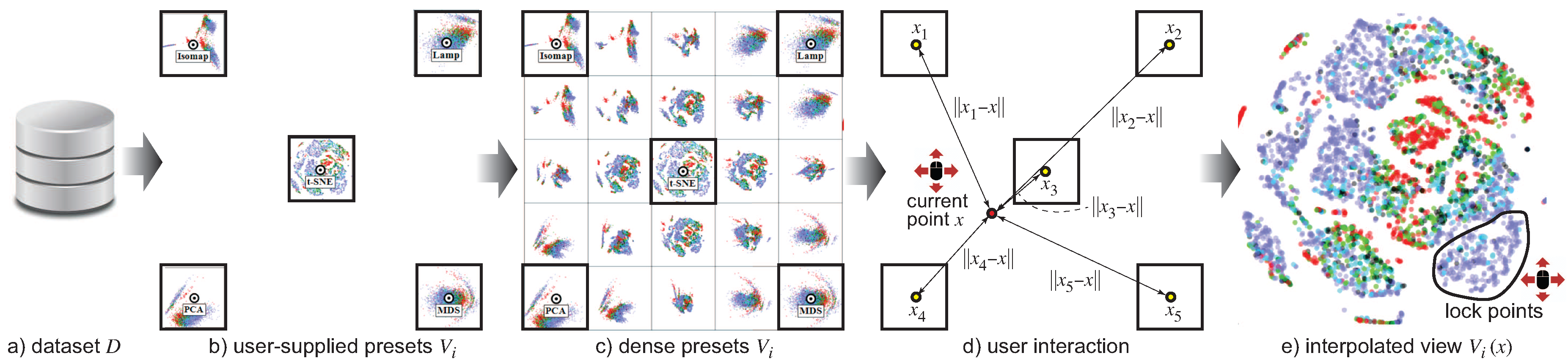
Figure 3.
Thumbnail grid and view interpolation. Each image shows a set of five preset views arranged on a five by five grid. The views are simple color pixels for illustration purposes. Each grid pixel is colored to reflect what the interpolated view would be at that position. (a) Initial placement of the preset views; (b) Effect of dragging the views along the arrows shown in (a); (c,d) Effect of setting and , respectively. The grids (a,b) use the default .

Figure 4.
(a–c) Three different types of navigation of the view space.
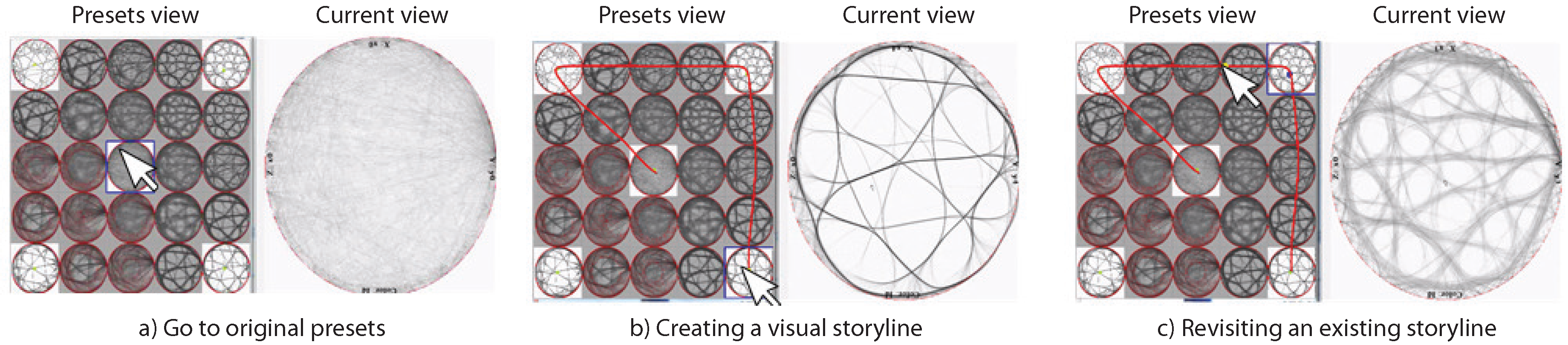
Figure 5.
Software quality dataset (Section 4.1.1). No projection in the view space is able to separate well repositories of one kind from those of other kinds.
Figure 5.
Software quality dataset (Section 4.1.1). No projection in the view space is able to separate well repositories of one kind from those of other kinds.

Figure 6.
Segmentation dataset (Section 4.1.2). Different views can separate well one or more of the classes, but no view succeeds this for all classes.
Figure 6.
Segmentation dataset (Section 4.1.2). Different views can separate well one or more of the classes, but no view succeeds this for all classes.

Figure 7.
Creating a mixed view which separates well the six classes present in the segmentation dataset.
Figure 7.
Creating a mixed view which separates well the six classes present in the segmentation dataset.
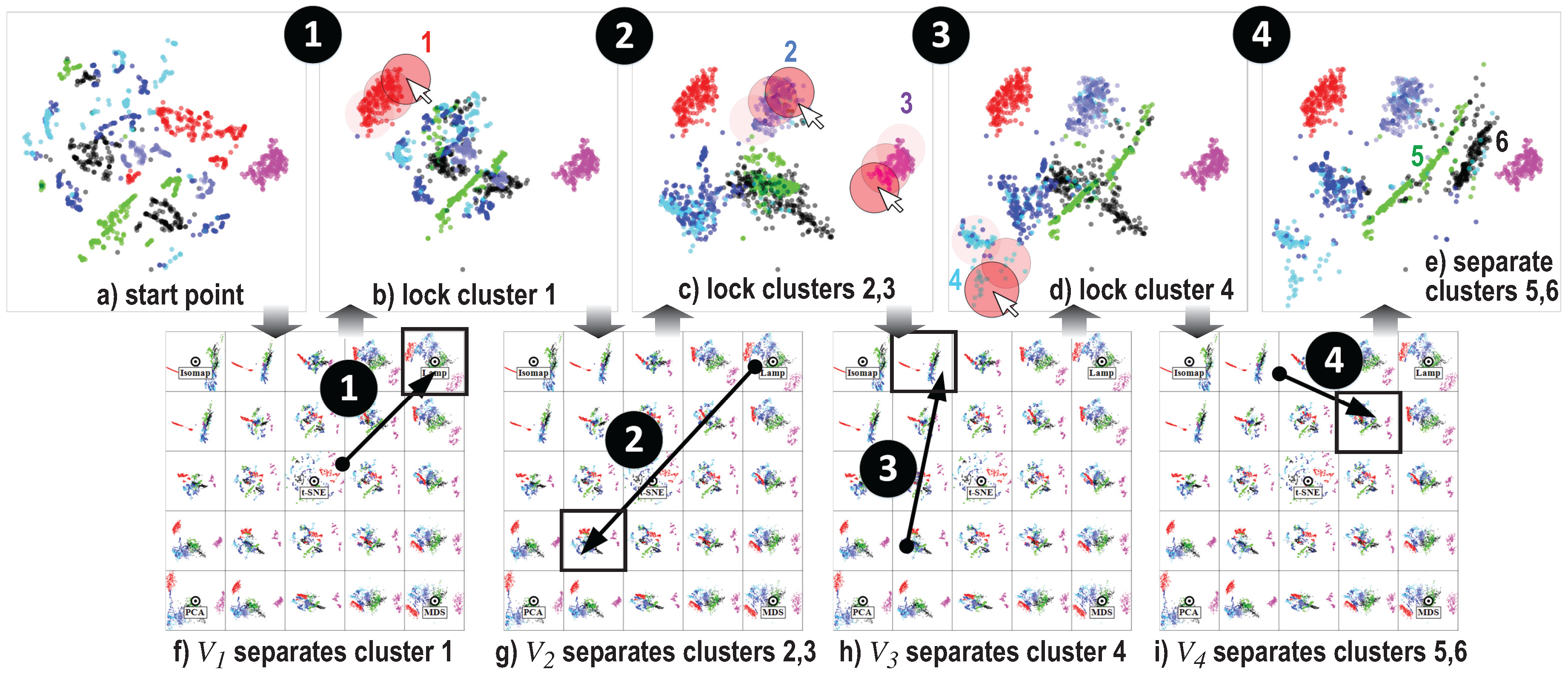
Figure 8.
Extracting relevant structures from four types of bundling algorithms to create a new bundling view for a graph dataset.
Figure 8.
Extracting relevant structures from four types of bundling algorithms to create a new bundling view for a graph dataset.
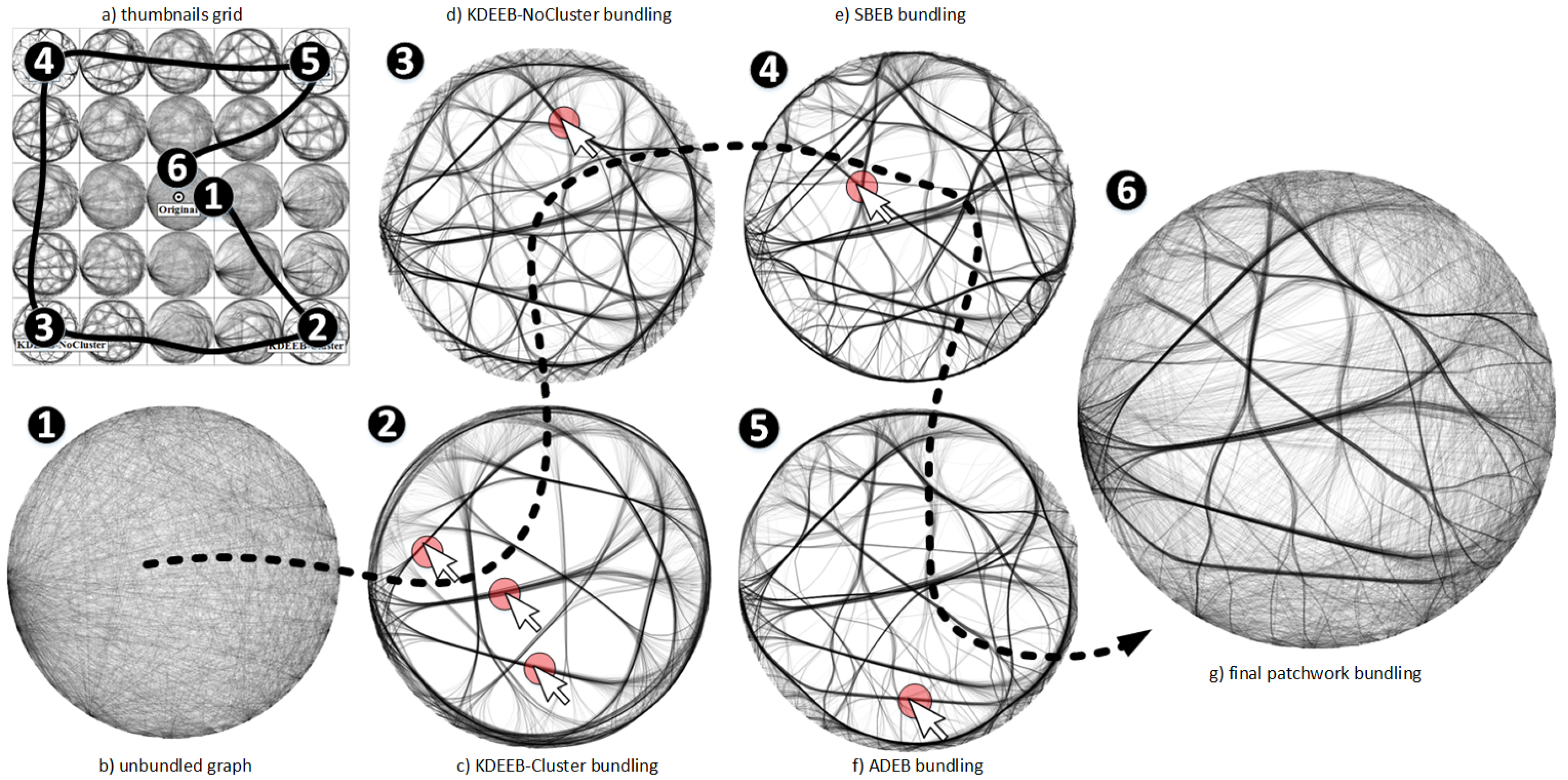
Figure 9.
Understanding differences between several EB techniques. The transition between KDEEB-cluster and any other technique produces fuzzy intermediate states (1 and 2), while the transition between SBEB and the othe techniques produces sharper images (3 and 4). This shows that KDEEB-Cluster is visually very different from the other clustering techniques considered.

Figure 10.
Bundling relaxation provided for four bundling techniques (presets in the corners of the grid) by our animation technique.
Figure 10.
Bundling relaxation provided for four bundling techniques (presets in the corners of the grid) by our animation technique.
© 2017 by the authors. Licensee MDPI, Basel, Switzerland. This article is an open access article distributed under the terms and conditions of the Creative Commons Attribution (CC BY) license (http://creativecommons.org/licenses/by/4.0/).
Share and Cite
MDPI and ACS Style
Kruiger, J.F.; Hassoumi, A.; Schulz, H.-J.; Telea, A.; Hurter, C. Multidimensional Data Exploration by Explicitly Controlled Animation. Informatics 2017, 4, 26. https://doi.org/10.3390/informatics4030026
AMA Style
Kruiger JF, Hassoumi A, Schulz H-J, Telea A, Hurter C. Multidimensional Data Exploration by Explicitly Controlled Animation. Informatics. 2017; 4(3):26. https://doi.org/10.3390/informatics4030026
Chicago/Turabian StyleKruiger, Johannes F., Almoctar Hassoumi, Hans-Jörg Schulz, AlexandruC Telea, and Christophe Hurter. 2017. "Multidimensional Data Exploration by Explicitly Controlled Animation" Informatics 4, no. 3: 26. https://doi.org/10.3390/informatics4030026
Note that from the first issue of 2016, this journal uses article numbers instead of page numbers. See further details here.